Strongly Charged, Flexible Polyelectrolytes
in Poor Solvents –
Molecular Dynamics Simulations
Uwe Micka, Christian Holm, and Kurt Kremer
Max-Planck-Institut für Polymerforschung
Ackermannweg 10
55128 Mainz, Germany
August 28, 1998

We present a set of molecular dynamics (MD) simulations of strongly charged, flexible polyelectrolyte chains under poor solvent conditions in a salt free solution. Structural properties of the chains and of the solutions are reported. By varying the polymer density and the electrostatic interaction strength we study the crossover from a dominating electrostatic interaction to the regime of strong screening, where the hydrophobic interactions dominate. During the crossover a multitude of structures is observed. In the limit of low polymer density strongly stretched, necklace like conformations are found. In the opposite limit of high polymer density which is equivalent to strongly screened electrostatic interactions, we find that the chains are extremely collapsed, however we observe no agglomeration or phase separation. The investigations show that the density of free charges is one of the relevant parameters which rules the behavior of the system and hence should be used as a parameter to explain experimental results.

PACS numbers: 61.25.Hq, 36.20.-r, 87.15.-v
E-mail: kremer@mpip-mainz.mpg.de, holm@mpip-mainz.mpg.de

1 Introduction

Unlike neutral polymers [1, 2, 3], the understanding of the behavior of electrically charged macromolecules, short polyelectrolytes, is still rather poor. The long range nature of the electrostatic interactions introduces new length and time scales that render the analytical description very complicated [4] and prevent simple scaling arguments to work equally successfully as in the neutral case. Usually, analytic theory [5] assumes $\theta$-properties for the uncharged monomers, while simulations use either $\theta$- or good solvent conditions [6, 7, 8, 9, 10]. Nevertheless, most experimentally relevant systems have organic, non-polar backbones in polar solvents (water) so that poor solvent conditions are more appropriate [12]. The analytic description of these systems is not far developed. In a first attempt, Dobrynin et al. [13] studied a single weakly charged chain under poor solvent conditions. Starting from the description of a charged drop, originally given by Lord Rayleigh in 1882 [14], their theory predicts that when the charge density or the strength of the electrostatic repulsion increases, the globular state becomes unstable and starts to split into smaller globules, which try to separate. Due to the covalent bonds the parts cannot dissociate completely. By maximizing their distance, they form structures which are called pearl-necklace chains.

The approach of Dobrynin et al. is supported by a Monte Carlo simulation of a single chain that shows a cascade from one to two and three globules with increasing strength of the electrostatic repulsion [13]. In their study every monomer carries a fractional charge, the polyelectrolyte is weakly charged and no explicit counterions are taken into account. Additionally to this previous Monte Carlo study, there exist some experimental evidence [16] supporting the picture of Dobrynin at al. A recent Monte-Carlo simulation of single Debye-Hückel chains near the $\theta$ transition also supports these findings [17]. However, there has been also put some doubt on the validity of this scheme in the case of discrete ions [18]. Our study will use many chains with discrete counterions, where the charges all interact via the full Coulomb potential, simulated wit molecular dynamics (MD).

Alternatively, a cylindrical instability was proposed by Khokhlov and his collaborators [19]. They argue that there will be a micro-phase separation due to a kind of agglomeration of the collapsed chains. This state would increase the entropy of the condensed counterions which could explore the whole volume of the phase separated chains. In an earlier short communication [20] we showed that based on simulational data no phase separation was observed and gave a simple argument for a stable colloid like state of single collapsed chains. In this article we will present in detail our simulations of polyelectrolytes in poor solvents. The rest of the paper is organized as follows: In section 2 we will describe our model, and show in section 3 the strong influence of the hydrophobic interaction, when it is put into a right proportion to the electrostatic interaction. In section 4 we will present the single chain properties of a polyelectrolyte under poor solvent condition, which shows indeed a cascade of pearl-necklace structures, if one varies the polymer density. We also explain why the colloid like state of the collapsed chain seems to be the stable one, and why no phase separation is observed. As last point in section 5 we compare our results to experimental data and suggest for future experiments those parameters which we consider to be the important quantities to vary.

2 Model

The polyelectrolyte chains are modeled as bead spring chains of Lennard-Jones (LJ) particles.

For good solvent conditions, a shifted LJ potential is used to describe the purely repulsive excluded volume interaction between all monomers:

$$U_{LJ,hydrophil}(r)=\begin{cases}4\cdot\epsilon_{LJ}[(\frac{\sigma}{r})^{12}-(\frac{\sigma}{r})^{6}]+\epsilon_{LJ}&\text{for }r\leq r_{min}=2^{\frac{1}{6}}\sigma\\ \hskip 27.03003pt0&\text{for }r>r_{min}=2^{\frac{1}{6}}\sigma\end{cases}$$ (1)

The parameter $\sigma$ is used to set the length scale. The energy parameter $\epsilon_{LJ}$ controls the strength of the interaction, and its value for the good solvent case is fixed to $\epsilon_{LJ}=1.0k_{B}T$, where $k_{B}$ is the Boltzmann constant and $T$ is the temperature. Polymers that are in good solvent and whose monomers interact via this potential are called “hydrophilic” for the rest of this paper. Although we do not have any explicit solvent and no specific potentials for the solvent water, we use this abbreviation because water is in experiments, technical applications, and nature the most common solvent for polyelectrolytes. As a consequence, particles under poor solvent conditions are called “hydrophobic”. Because we do not consider any explicit interactions between solutes and solvent molecules one way to model poor solvent conditions is through an additional attractive interaction between the chain monomers.

We represent this potential by a standard LJ potential with a larger cut-off ($R_{c}=2.5\sigma$):

$$U_{LJ,hydrophob}(r)=\begin{cases}4\cdot\epsilon_{LJ}[(\frac{\sigma}{r})^{12}-(\frac{\sigma}{r})^{6}-c(R_{c})]&\text{for }r\leq R_{c}\\[2.84544pt] \hskip 27.03003pt0&\text{for }r>R_{c}\\ \end{cases}$$ (2)

The function $c(R_{c})$ is chosen as $c(R_{c})=(\frac{\sigma}{R_{c}})^{12}-(\frac{\sigma}{R_{c}})^{6}$ to give a potential value of zero at the cutoff. This potential is used only for chain beads, because we assume that the counterions do not have any hydrophobic parts in their interaction, as is reasonable for alkali metals, and describe their interaction by equation 1.

The connectivity of the bonded monomers is assured by the FENE (finite extension nonlinear elastic) potential:

$$U_{\rm FENE}(r)=-\frac{1}{2}k_{\rm FENE}R_{0}^{2}\ln(1-\frac{r^{2}}{R_{0}^{2}})$$ (3)

where $r$ is the distance of the interacting particles. The parameters are set the following way: the spring constant $k_{\rm FENE}=7.0\frac{k_{B}T}{\sigma^{2}}$ and $R_{0}=2\sigma$. $R_{0}$ gives the maximum extension of the bond, at which the interaction energy becomes infinite. This potential gives rather stiff bond lengths with fluctuations being smaller than 10 %. The nonlinearity allows a very efficient mixing of the different vibrational modes.

The Bjerrum length is a measure of the strength of the electrostatic interaction, which is defined as the length at which the electrostatic energy equals the thermal energy:

$$\lambda_{B}=\frac{e^{2}}{4\pi\epsilon_{S}\epsilon_{0}k_{B}T},$$ (4)

where $e$ is the unit charge of the interacting particles, and $\epsilon_{0}$ and $\epsilon_{S}$ are the permittivity of the vacuum and of the solvent, respectively ($\lambda_{B}=7.1$Å in water). Here we restrict ourselves to monovalent species in salt free solution. The solvent is taken into account via the dielectric background, whose properties influence the form (hydrophil or hydrophob) of the interaction potential of the monomers. Unless mentioned the Bjerrum length is always fixed to $\lambda_{B}=3.0\sigma$.

No assumptions concerning screening effects are made, instead we are using the pure Coulomb energy to calculate the interactions between all charged particles:

$$E^{Coul}(r_{ij})=k_{B}T\frac{\lambda_{B}q_{i}q_{j}}{r_{ij}},$$ (5)

where $q_{i}=+1$ for the charged chain monomers, and $q_{i}=-1$ for the counterions, which are treated explicitly as charged LJ particles.

The central simulation box contained 16 or 32 chains subject to periodic boundary conditions. Each chain consisted of 94 monomers. The fraction $f$ of charged monomers on the chain is $f=\frac{1}{3}$, meaning that every third monomer carries a unit charge. We also put a charge on the chain ends, hence the number of charges per chain is always 32. A velocity Verlet algorithm is used to integrate the equation of motion. The system is coupled to a thermostat via a standard Langevin equation with a friction term and a stochastic force. The friction coefficient $\Gamma$ is set to $\Gamma=\tau^{-1}$ and the time step $\Delta t$ varies between $\Delta t=0.003\tau$ and $0.0125\tau$ depending on $\epsilon_{LJ}$, where $\tau$ is the standard LJ time unit [7]. Because of the periodic boundary conditions the Coulomb interaction is calculated with a fast variant of the Ewald summation [21], the Particle-Mesh-Ewald (PME) algorithm [22] in the version presented by Petersen [23]. The basic idea is to calculate the Fourier part of an Ewald summation with a Fast Fourier Transform on a mesh to speed up the calculation. Our version is more efficient than the highly optimized version of the Ewald sum of Ref.[7] if more than 800 charges are simulated. The parameters of the PME method were always chosen such that the resulting errors in the electrostatic forces were well below the random forces produced by the Langevin heat bath. At the time of the production of our data this method was the only mesh based Ewald sum, for which analytic error estimates [23] were available. Note, however, that meanwhile a better method, also with analytic error estimates, is available [24].

Our polyelectrolyte systems are strongly charged. By this we mean that the Manning parameter which is defined as the Bjerrum length divided by the length per unit charge, $\xi_{M}=\frac{\lambda_{B}}{3b}$, is close to the critical value. The critical Manning parameter, at which counterion condensation is commonly expected to set in, is equal to $\xi_{M}^{*}=1$ for monovalent counterions. In our simulation, the average bond length is given by $b\approx 1.08\sigma$, leading to $\xi_{M}\approx 0.927$, so that we are just below $\xi_{M}^{*}$, therefore the expression “strongly” charged.

Our model polyelectrolyte system can be mapped to the “standard polyelectrolyte” sulfonated polystyrene (PSS), as can be seen for instance from the Manning parameter. A PSS-monomer extends over roughly $2.5$Å and the Bjerrum length in water is about $7.1$Å leading to about one charge per three monomers. Each chain contains 94 monomers meaning 32 charges and models a molecular weight of roughly 20.000 $\frac{\text{g}}{\text{mol}}$, if a sodium counterion is assumed. This molecular weight, though not very large, is well within the experimentally analyzed regime [12].

A crucial parameter in the simulations will be the concentration of particles in the simulation box of length $L$. No difference will be made between counterions, charged and uncharged monomers because they are all Lennard-Jones-particles. This concentration will be called density for the rest of this paper and therefore be denoted by $\rho$. By varying the box length $L$ we can vary the density from $2\cdot 10^{-1}\sigma^{-3}$ to $2\cdot 10^{-6}\sigma^{-3}$, which is covering more than the whole experimentally accessible range from very dense to extremely dilute solutions.

3 Influence of the hydrophobic interaction strength

To characterize the hydrophobicity of a polyelectrolyte chain one has to develop a measure for the relative strengths of the hydrophobic and the electrostatic interaction. The strength of the electrostatic interaction is determined by $\lambda_{B}$. The attractive interaction in Lennard-Jones systems (as for instance neutral polymers) is usually tuned by variation of the temperature $T$. The aim of the present work is to study the influence of the poor solvent with fixed boundary conditions (constant $\lambda_{B}$ and constant $T$). For the case of polyelectrolytes a variation of the temperature in the simulations changes simultaneously the strength of the electrostatics for fixed $\lambda_{B}$. For this reason, the hydrophobicity is varied by changing the parameter $\epsilon_{LJ}$ in the LJ potential (2) as an independent variable. We fix the energy scale by setting the thermal energy equal to $k_{B}T=1.0$. In a simulation this is a common way to separate and isolate effects. We are well aware of the fact that in experiments a change of temperature influences in a rather complex manner all relevant quantities.

In order to make contact with neutral polymer theory the $\theta$ point for the neutral polymer system has to be determined first. The $\theta$ point is usually defined by the temperature at which the second virial coefficient between the chains vanishes. There the attractive and repulsive interactions cancel up to second order, so that the polymers show (almost) ideal random walk behavior. For the underlying neutral LJ system only a crude estimate for the $\theta$ point has been found so far in Ref. [25]. The temperature $T_{\theta}^{(n)}$ and the LJ energy parameter $\epsilon_{LJ}^{(n)}$ of this point were determined as $T_{\theta}^{(n)}\gtrsim 3.0\pm 0.2$ for $\epsilon_{LJ}^{(n)}=1.0$. Converted to our notation this is equivalent to a value of $\epsilon_{LJ,\theta}^{(n)}\leq\frac{1}{3}$ at a thermal energy $k_{B}T=1$. To get a more precise estimate on the location of the $\theta$ point we therefore employed a scaling approach that was shown to be very successful for polymers and star-polymers on a face-centered cubic lattice (fcc) [26]. This approach utilizes that the end-to-end distance can be expressed as:

$$R_{end}^{2}=\text{N}\cdot g(\tilde{T}\cdot\text{N}^{\frac{1}{2}}),$$ (6)

where $g$ is an unknown scaling function, and $N$ is the number of monomers of a chain. The argument $\tilde{T}=\frac{T-T_{\theta}}{T_{\theta}}$ describes the reduced distance to the critical point. This relation is easily translated to an $\epsilon_{LJ}$-dependent formula. The main point is that for fixed values of the ratio $\frac{R^{2}_{end}}{N}$ the argument of the scaling function must be also fixed. It follows that

$$\tilde{T}\sim\text{N}^{-\frac{1}{2}}$$ (7)

Plotting T versus $N^{-\frac{1}{2}}$ for fixed ratio of $\frac{R^{2}_{end}}{N}$ results in straight lines that should converge to the $\theta$ point for $N^{-\frac{1}{2}}\rightarrow 0$, neglecting some deviations due to statistical errors and higher order corrections to scaling. Neutral chains from $N=32$ up to $N=2048$ monomers were studied. The scaling plot can be viewed in Figure 1, showing that the effective interaction parameter for $\theta$ conditions is given by $\epsilon_{LJ,\theta}^{(n)}=[2.96\pm 0.06]^{-1}=0.34\pm 0.02$.

Based on this information for the neutral system three simulations of the charged system were performed at a fixed density of $\rho=10^{-4}\sigma^{-3}$, but for the three different values $\epsilon_{LJ}=0.25$, $0.5$, and $1.0$. While $\epsilon_{LJ}=0.25$ is well above the neutral $\theta$ point, where a behavior similar to the hydrophilic system can be expected, $\epsilon_{LJ}=0.5$ should show some signs of the hydrophobic influence. For that reason, the system with $\epsilon_{LJ}=0.5$ will be called “weakly hydrophobic” for the rest of the paper, while the system with $\epsilon_{LJ}=1.0$ is deep in the hydrophobic regime.

We first looked at the spherically averaged structure factor of a single chain

$$S_{sp}(q)=\left\langle\frac{1}{{\rm N}}\left|\sum_{i<j}^{{\rm N}}\exp(i\vec{q}\cdot(\vec{r}_{i}-\vec{r}_{j}))\right|^{2}\right\rangle$$ (8)

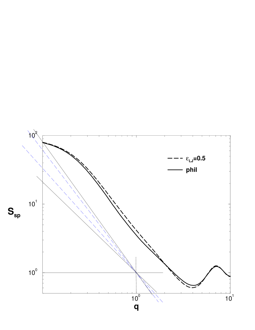
Figure 4: The spherically averaged structure factor $S_{sp}(q)$ vs. $q$ for hydrophilic (phil) and weak hydrophobic ($\epsilon_{LJ}=0.5$) chains for the density $\rho=10^{-1}\sigma^{-3}$. The dashed straight lines indicate the slope of the linear part of the hydrophobic data, the solid lines that one of the hydrophilic data.

and its component along the first principal axis of inertia, $S_{\parallel}$, which is obtained by restricting the $\vec{q}$ - vectors to the direction of the calculated principal axis. The values for $S_{sp}(q)$ and $S_{\parallel}(q)$ are displayed in the top and bottom part of Figure 2, respectively, where it is found that all three of these systems are very similar and do not differ significantly from the known behavior of hydrophilic polyelectrolytes. Because the charge density strongly influences the screening of the electrostatic interactions, the comparison of charged systems for different values of $\epsilon_{LJ}$ is extended over a whole range of densities. In Figure 3 the radius of gyration $R_{G}$ is displayed versus various densities. The attractive potentials cause locally more compact conformations, leading to smaller $R_{G}$, which can also be seen in Figure 4, where the spherically averaged structure factor is displayed for $\rho=10^{-1}\sigma^{-3}$.

The main results of these preliminary investigations show, that the electrostatic interaction is still too strong compared to the influence of the hydrophobicity. However, under certain conditions, even the “weak” hydrophobicity has pronounced effects.

One of theses conditions is the relative strength of the electrostatic interaction. The strength of the Coulomb interaction can be conveniently altered by varying the Bjerrum length $\lambda_{B}$. It is well known that if one increases $\lambda_{B}$ by starting from small values, this will lead to a non-monotonic behavior of the chain dimensions [7], which is due to counterion condensation[27, 28, 29].

The basic idea of counterion condensation is a generalization of the well known solution of Onsager [30] for the infinitely long and thin line charge. If the energy density on the rod exceeds a certain value it becomes more favorable to catch one of the free ions to neutralize one of the charges on the chain. The calculation results in the condition that the distance between two adjacent unit charges on the chain has to be bigger than $\lambda_{B}$, which means that their mutual pure Coulomb repulsion energy has to be smaller than $k_{B}T$. For that reason, the entropy of the counterion, that is lost in the condensation process, is assumed to equal $k_{B}T$. By analogy, this argument is applied to any (flexible) polyelectrolyte, which is, however, questionable. We define a counterion as condensed, if its total energy is smaller than $-1k_{B}T$. This way is easy to handle and strongly supported by a visual inspection of the set of condensed counterions of our conformations. It has some advantages over the geometrical definition, where one looks at the distance of a counterion to its nearest polymer, and sets some arbitrary bound, because an ion can feel a strong attraction to several charged monomers even at a relatively large distance.

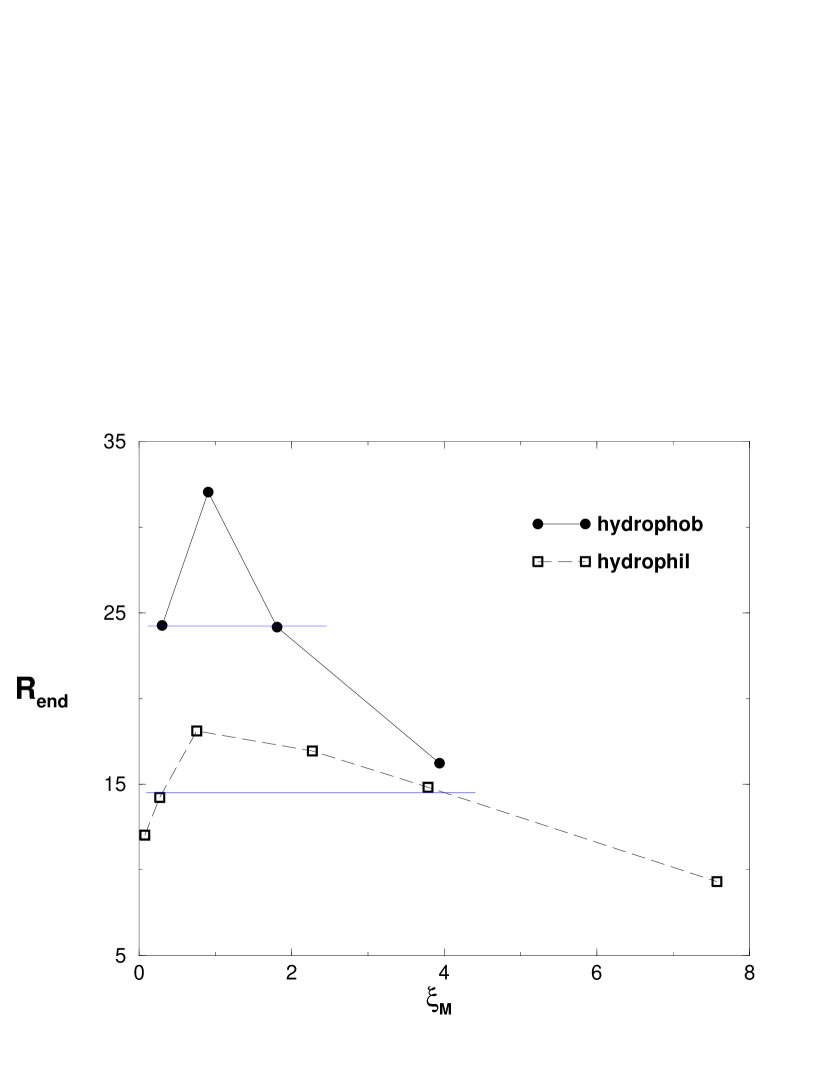
Figure 5: End-to-end distance $R_{end}$ as a function of the Manning parameter $\xi_{M}$ for hydrophilic chains ($\epsilon_{LJ}=0.25$, $\Box$, from Ref. [7]), and hydrophobic chains ($\epsilon_{LJ}=0.5$, $\bullet$). The straight line indicates comparable end-to-end distances.

The results of Ref.[7] and our new data show that first, increasing $\lambda_{B}$ stretches the chains through the increased repulsion of the equally charged chain monomers. Then a maximum is reached and the chains start to contract, due to counterion condensation, which decreases the effective charge on the chain. When the Bjerrum length is further increased, eventually all counterions condense, and then the collapsed chains will start to coagulate forming a liquid sol and droplet. This was later also observed in Ref. [31]. Because the hydrophobic polyelectrolytes have an additional attractive force between the monomers, a reduction of the chain extensions occurs already for lower $\lambda_{B}$, and this contraction will be stronger than in the hydrophilic case. Figure 5 reflects exactly this behavior, where we compare the end-to-end distances $R_{end}$ for the two cases $\epsilon_{LJ}=0.25$ and $\epsilon_{LJ}=0.5$ as a function of the Manning ratio $\xi_{M}$ at a density of $\rho=2\cdot 10^{-2}\sigma^{-3}$. The data for the hydrophilic polyelectrolytes is taken from Ref. [7]. where the model contained no explicit neutral monomers, so we can not compare the absolute values. For our purposes, however, a comparison of the tendencies is sufficient. In Figure 5 one recognizes that the hydrophobic system contracts to a radius that is a factor of two smaller at $\xi_{M}=3.94$! The relative contraction of the hydrophilic chain compared to the reference state is only about 30% at $\xi_{M}=7.58$. These values clearly show that already the influence of weak hydrophobicity changes drastically the conformational properties of polyelectrolytes.

Further evidence for this can be gained from the number of condensed counterions as a function of the Bjerrum length $\lambda_{B}$, displayed in Figure 6. It increases from 12 to 29 around $\lambda_{B}\approx 3$ ($\xi_{M}\approx 1$) showing exactly the dramatic effect as argued above and in reference [7]. An analysis of the structure factor at the very high Bjerrum length of $\lambda_{B}=13\sigma$, compare Figure 7, gives further evidence that the conformation is in a collapsed state.

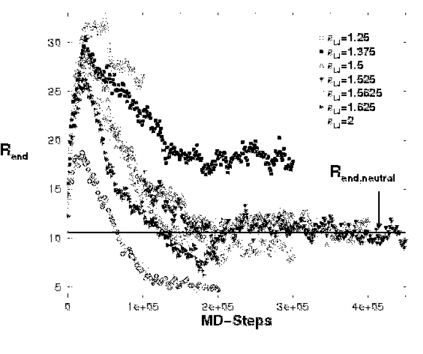
Figure 8: Time development in MD steps of the end-to-end distance $R_{end}$ of charged chains for various hydrophobicities $\epsilon_{LJ}$. The straight horizontal line indicates the end-to-end distance of the equally long uncharged random walk

As seen above, even at a value of $\epsilon_{LJ}=1.0$ the chain conformation at $\rho=10^{-4}\sigma^{-3}$ was not significantly altered although the neutral chain would be strongly in the hydrophobic regime. For that reason, we found it necessary to compute an “effective” $\theta$ point for the charged system in the following way: The end-to-end distance $R_{end}$ is calculated as a function of $\epsilon_{LJ}$. The effective $\theta$ point is then defined by the value of $\epsilon_{LJ,\theta_{eff}}^{(c)}$ at which $R_{end}$ equals the one for an ideal neutral chain of this length. The $\theta$ point is called effective, because it is determined only for the system under consideration, and hence is not an asymptotic statement. Figure 8 shows the time development of $R_{end}$ for different $\epsilon_{LJ}$ at the fixed density $\rho=10^{-4}\sigma^{-3}$. From the data the relevant parameter $\epsilon_{LJ,\theta_{eff}}^{(c)}$ is determined to be

$$\epsilon_{LJ,\theta_{eff}}^{(c)}\simeq 1.51\pm 0.03.$$ (9)

Polymers with this parameter will be henceforth called “strongly hydrophobic”. Starting from this value of $\epsilon_{LJ,\theta_{eff}}^{(c)}$, dominating hydrophobicity at higher densities and dominating electrostatics at lower densities will be observed in the next section.

4 Variation of the density - single chain properties

Our intention in this section is to study the crossover from strong screening to dominating electrostatic interaction by changing the polymer density $\rho$. The Bjerrum length is fixed to $\lambda_{B}=3.0\sigma$, $k_{B}T=1$ and the strength of the hydrophobicity is set to $\epsilon_{LJ}=1.5$ in light of the results of the previous section. 16 chains of length $N=94$ are simulated for densities varying from $\rho=2\cdot 10^{-1}\sigma^{-3}$ to $\rho=2\cdot 10^{-6}\sigma^{-3}$.

First we want to start by comparing a hydrophilic system to the weakly hydrophobic one, $\epsilon_{LJ}=0.5$, and to the strongly hydrophobic system with $\epsilon_{LJ}=1.5$. Especially noteworthy is the similarity between the weakly hydrophobic and the hydrophilic system, and the strong contrast of both systems to the strongly hydrophobic system. On a very local scale there is no large difference in all three systems as a function of density. This is reflected in Figure 9 that shows the average bond length. The differences in the total values are due to the slight differences in the repulsive part of the LJ potentials with different $\epsilon_{LJ}$. As this difference is only small and completely irrelevant for the rest of the investigation, we did not correct for it, e.g. by an adjustment of the FENE potential.

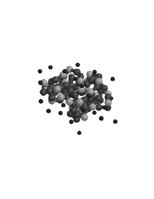
Figure 11: Conformations at the density $\rho=2\cdot 10^{-2}\sigma^{-3}$. Top: A typical poor solvent polyelectrolyte conformation. The beads are the charged monomers, the counterions are indicated as small black spheres, and the neutral monomers are dark grey spheres. Only counterions within a distance of $3\sigma$ to the chain are displayed. Bottom: A snapshot of the whole simulation box, showing all 16 chains together with their counterions. The picture shows that the chains collapse into single globules which are well separated, and a small fraction of the counterions is still in solution.

Much more interesting is the behavior of the end-to-end distance $R_{end}$ and the characteristic ratio $r=\frac{R^{2}_{end}}{R^{2}_{G}}$. As already presented elsewhere [20] the hydrophilic system stretches for decreasing density from a starting point well above the self-avoiding-walk value. The hydrophobic chains pass through a pronounced minimum at $\rho=2\cdot 10^{-2}\sigma^{-3}$. Both observables can be inspected as a function of density in Figure 10. The characteristic ratio $r$ is known to equal six for a random walk, 12 for a rod and is supposed to be around 6.3 for a self avoiding walk. For a homogeneous sphere, with the ends randomly distributed over the volume, $r=2$, and $r=10/3$, if the ends are constraint to be randomly distributed on the surface [17, 20]. For deformed collapsed chains we thus expect a value well below $r=6$ but above $r=10/3$. For the density $\rho=2\cdot 10^{-2}\sigma^{-3}$ we find a value of $r=4.68$, meaning that the system is in a strongly collapsed state. A typical conformation for that density and the snapshot of the whole box can be viewed in Figure 11.

At the highest density $\rho=0.2\sigma^{-3}$, where the electrostatic interaction is even weaker, the chains are not collapsed completely. However, the density is so high that strong intermolecular hydrophobic forces cause the system to collapse into a gel-like object, as can be inspected in Figure 12, where every chain is interpenetrated by several others. The conformations of the single chains are dominated by the topological constraints imposed by neighboring chains, and we find a broad spectrum of shapes. A simple screening argument for the electrostatic and the excluded volume interaction can not explain the increase in size, because the density is still too low. However, there might also be problems connected with the simulation of a quasi-stable (eventually also in experiment “glassy”) state. For these higher densities, there is almost no energetic advantage to collapse in well separated single molecules any more. Figure 13 shows a typical representative of the dominant conformations. It is clearly less collapsed than the chain at the lower density in Figure 11. This can also be observed more clearly in the single chain structure factor. A collapsed chain should have a chain length dependence of $R_{end}$ that scales with an exponent $\nu=\frac{1}{3}$ which leads to a decay of the spherically averaged structure factor with a slope of $m=-3$. This is roughly seen in the data set at $\rho=0.2\sigma^{-3}$. For $\rho=2\cdot 10^{-2}\sigma^{-3}$, however, a value of $m=-4$ is found that is characteristic for Porod scattering at distinct phase boundaries [32]. This demonstrates how extreme the chain collapse is, as can be inspected in Figure 14. For lower densities the slope converges towards $m=-2$, which is the random walk value. Nevertheless, this value has to be taken with care, because the attractive forces will prevent one from observing a real random walk behavior. Additionally, the linear range in the log-log plot of Figure 14 is rather small.

We have found that the collapse of the system into a microgel, or isolated chains, is just a consequence of a strongly hydrophobic attraction in polyelectrolytes. Because the simulated densities were rather high, this effect should be easily observed in experiments. Especially the isolated chains should be a very interesting candidate to study, because they still interact strongly via electrostatic interactions. As Figure 11 shows, they should behave like a solution of charge stabilized colloidal particles. Nevertheless, the internal degrees of freedom will always play a very important role in polyelectrolytes and distinguish them from charged colloids.

The stability of the colloidal phase can be inferred by the following simple estimates[20]. We start to determine the number of condensed ions in order to get the net charge of the collapsed object. The results are plotted in Figure 15. We find that 26 ions are condensed at $\rho=2\cdot 10^{-2}\sigma^{-3}$ leading to a net charge of 6 per chain. This coincides very nicely with the number which one obtains from the critical charge $Q$ for a charged drop according to the Rayleigh criterion, where one balances the Coulomb energy $E^{Coul}(R_{G})=\lambda_{B}k_{B}TQ^{2}/R_{G}$ with its surface energy $E^{surf}(R_{G})=4\pi R_{G}^{2}k_{B}T/A_{surf}$. If one uses for the surface area $A_{surf}$ the monomer area $\pi b^{2}$, one gets for the critical charge the formula

$$Q^{2}=\frac{4R_{G}^{3}}{b^{2}\lambda_{B}}.$$ (10)

Using the values $b=1.08\sigma$ and $R_{G}=3.2\sigma$, valid for the density $\rho=2\cdot 10^{-2}\sigma^{-3}$, one finds $Q\approx 6.1$. Of course the number of condensed counterions strongly increases with density, because the screened electrostatic interaction cannot stretch the chains any longer. These more compact states have to be stabilized by the oppositely charged counterions. Their entropy loss is overcome by the energy gain in the chain. In Ref. [20] a simple free energy argument was presented to show that the colloidal phase (1c) is more stable than a hypothetical agglomerate of two chains (2c). The critical charge $Q_{2c}$ for the agglomerate of two chains for the same density $\rho=2\cdot 10^{-2}\sigma^{-3}$ is found with Eq.(10) by using $(R_{G})_{2c}=R_{G}2^{1/3}=4.0\sigma$ to take on the value $Q_{2c}\approx 8.7$. Therefore, in order for two chains to agglomerate an additional number of 3.5 counterions have to condense on average onto the pair of chains which carry each an average charge of $Q_{c1}=6.1$. To estimate the free energy difference of the two globular states, one needs to look only at the Coulomb energy of the globules with each other and the entropy of the remaining counterions in solution, because the intra Coulomb energy and the surface energy are already balanced from the Rayleigh criterion (10). Assuming a uniform distribution of the chains in the simulation box, we find the distances $d_{1c}=18.5\sigma$ and $d_{2c}=23.3\sigma$ for the one chain and two chain globular state, respectively, to their next neighbors. The repulsive Coulomb energy between two neighboring chains is given by

$$E^{Coul}=\lambda_{B}k_{B}T\frac{Q^{2}}{d}.$$ (11)

To make the calculation simple we assume the chains to sit on a simple cubic lattice. We also neglect higher multi-pole moments and take only the next neighbor chains into account. The influence of the counterions is also ignored, because on the average only one is available per neighbor. With these simplifications the average Coulomb interaction energy per single chain is found to be $E^{Coul}_{1c}=18.1k_{B}T$/chain and $E^{Coul}_{2c}=14.6k_{B}T$/chain, respectively. The corresponding value for an agglomerate of two chains is therefore about $3.5k_{B}T$ lower, preferring the agglomerate. The entropy of the free counterions can be approximated by an ideal gas Ansatz. The free counterion densities are given by $\rho_{1c}=6.1/(94+32)\rho$ and $\rho_{2c}=4.35/(94+32)\rho$, respectively. Because the entropy per free ion is given by the logarithm of the available volume fraction the entropic contribution of the free energy difference per single chain is given by $6.1\ln\rho_{1c}-4.35\ln\rho_{2c}\approx-10.7k_{B}T$. This gives a total preference of $7.2k_{B}T$/chain for the single chain globule[20].

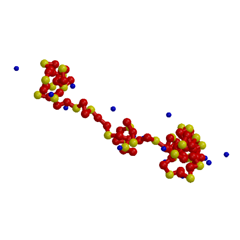
Figure 17: A typical poor solvent polyelectrolyte conformation for the density $\rho=2\cdot 10^{-5}\sigma^{-3}$, which shows nicely a pearl-necklace structure. The coloring is as in Fig. 11

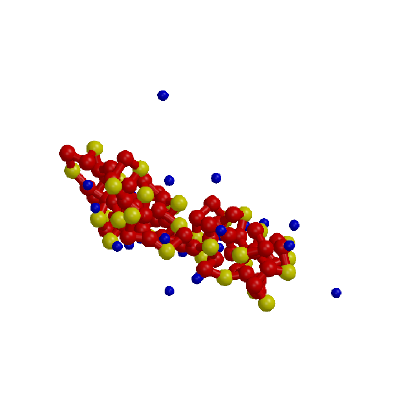
Figure 19: A typical poor solvent polyelectrolyte conformation for the density $\rho=2\cdot 10^{-3}\sigma^{-3}$. One sees the onset of the Rayleigh instability, the globule wants to split up into two parts. The coloring is as in Fig. 11.

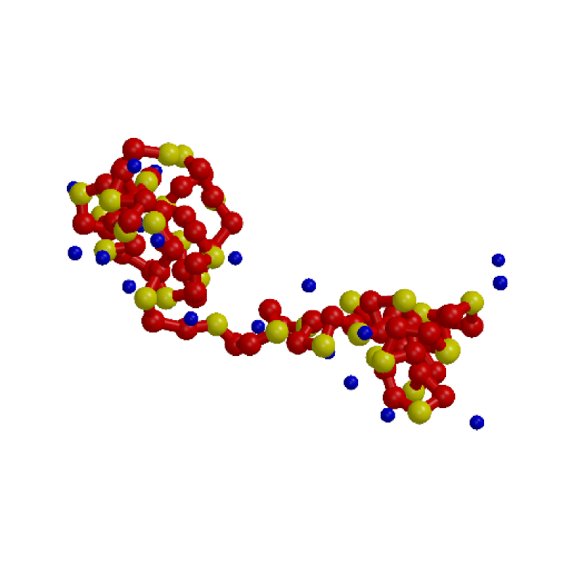
Figure 20: A typical poor solvent polyelectrolyte conformation for the density $\rho=2\cdot 10^{-4}\sigma^{-3}$, where now two globules with a bridge connecting them, has formed . The coloring is as in Fig. 11

The spherically averaged single chain structure factor shows another very striking feature at low $q$, this time for the lowest densities. At $\rho=2\cdot 10^{-5}\sigma^{-3}$ and $\rho=2\cdot 10^{-6}\sigma^{-3}$ a second well defined length scale shows up. The logarithmic slope measured is exactly $m=-1$, as can be seen in Figure 16, which corresponds to an exponent $\nu=1$. This is an extraordinary result, because no other polymeric systems show such a behavior. For example, hydrophilic polyelectrolytes always have an exponent $\nu<1$, because entropic fluctuations lead to some local roughness[7]. Even the blob pole conformations observed in simulations of single Debye-Hückel chains [6] that show a linear dependency of the end-to-end distance on the contour length after introduction of the concept of electrostatic blobs, show an effective exponent $\nu$ smaller than one. Figure 17 and 18 show typical pearl-necklace like conformations. Small globules are connected by thin bridges. The stronger the electrostatic interactions are, the larger is the number of globules. The globules are in addition stabilized by a few condensed counterions. So we can qualitatively reproduce the picture of Ref. [13] for our strongly charged systems. Of course, the globules are much smaller than in their weakly charged case, but clearly detectable. The chains are strongly stretched due to the electrostatic interaction which orients the different globules to an almost rodlike object by maximizing their mutual distance. Additionally, the chains are, at least within the globules, locally not very flexible, because the monomers dislike to break the energetically favorable hydrophobic bonds (around $E=1.5k_{B}T$ per contact). To complete the set of pictures of conformations, we display in Figures 19 and 20 typical conformations at intermediate densities. A continuous deformation towards a dumbbell like conformation is observed, but no cylindrical instability is found. It is interesting to note, that the larger globules are found at the chain ends, and the smaller ones reside in the chain middle.

At the end of this section we want to stress again, that no micro-phase separation is observed, although this is theoretically predicted [19]. Only for the highest density we can not rule out that this will eventually happen. The main argument for a micro-phase separation was that the entropy of the condensed counterions in the polyelectrolyte-rich phase is much larger, because the condensed counterions can explore the whole volume of the separated phase. We have been showing in our previous communication [20], that the system prefers single chain globules, which repel each other because they still have a sufficiently high net charge. Additional counterions would need to condense to stabilize an agglomerate of two or more chains. However, their loss of translational entropy (and the increase in Coulomb energy) is much larger than the gain in surface energy, and therefore single, isolated globules are clearly favored in certain density regimes.

5 Comparison with experiments

It is important to try to compare these results to experimental data. Unfortunately, most experiments do not examine single chain properties with adequate precision. Especially for low densities, where the mutual influence of the chains can be neglected, scattering experiments are extremely difficult. A comparably new experimental study [16] shows good agreement with our data at relatively high densities. Unfortunately, the density was only varied once by a factor of two, so that the effects we report in this paper, could not be seen.

Most experimental results come from detailed measurements of the structure factor of the whole sample or thermodynamic properties like the osmotic pressure $\Pi$ are measured. To compare our results of section 4, however, data of single chain properties are needed, which unfortunately are rare. The structure factor of the whole simulation box that reflects the arrangement of the chains in space, is difficult to determine from the simulation data for the present poor solvent situation. The reasons are of technical nature. The structure factor itself can easily be calculated, however it is strongly influenced by finite size effects, as the number of chains in the simulation box is relatively small (16 or 32). The collapsed chains can see each other only weakly, which results in broad maxima in the pair-correlation function and in $S(q)$, which was not the case for the hydrophilic systems [7]. Nevertheless, the simulations are able to show some important aspects, which can help to interpret the experimental results, as will be shown below.

Experimentally, the maximum of the structure factor, which is the Fourier transform of the monomer pair correlation function of all monomers in the sample, shows a concentration dependent position $q_{max}\sim\rho_{c}^{\nu_{sf}}$ with $\nu_{sf}={\frac{1}{2}}$ at high densities and $\nu_{sf}={\frac{1}{3}}$ at low densities, where $\rho_{c}$ denotes the charge concentration. Because the statistical fluctuations are too high, a reasonable distinction between the relevant exponents (0.5 to 0.3) can not be given in our case. At low densities the scattering should reflect nothing but the distances between the uniformly distributed chains. These distances vary with $\rho^{-1/3}$. At higher densities the scattering results from the correlation hole that is supposed to be proportional to the screening length which then is proportional to the square root of the charge concentration [7, 15, 16].

For hydrophobic polyelectrolytes deviations of this behavior are found in small angle neutron and x-ray scattering experiments [16, 33]. An effective exponent of $\nu_{sf}=0.4$ is observed, while the hydrophilic chains show the usual exponent $\nu_{sf}=0.5$. The investigated hydrophilic polymer is strongly charged and seems to follows the Manning criterion over the examined small density range. So the charge is “fixed”, meaning the number of free charges in the system remains constant. In the following we argue that the number of free charges in the system is the relevant parameter to explain the experimental results. In Figure 15 the number of condensed counterions was plotted, which showed a strong density dependence. Because every condensed counterion neutralizes effectively one charged monomer, this will lead naturally to a reduced charged density at higher mass densities. The calculation of the screening length based on this “effective” charge density reproduces the smaller exponents quite well. Only at the highest densities, where the number of condensed counterions is almost constant, the exponent is given by the volume change and equals $\nu_{sf}=0.5$. In Table 1 and 2 we estimate the effective hard sphere diameter of the chains by calculating the DH radius. We assume that screening is only facilitated by the mobile, non-condensed counterions with a density $\rho_{fc}$. This defines a screening length $\kappa^{-1}=(4\pi\lambda_{B}\rho_{fc})^{-1/2}$. If we assume that the solution is in a liquid of hard spheres of radius $\kappa^{-1}$ and if we further assume that the effective particles are certainly big enough to interact, than we can argue that the effective exponent $y$, obtained via $\kappa^{-1}\propto\rho^{y}$ as given in Tables 1 and 2 should reflect the experimental data for the scattering. There is however a word of care needed. The value of $\nu_{sf}=0.5$ as given from scaling assumes a blob picture with strongly interacting chains. Thus this cannot expected to hold so easily here. On the other hand for hydrophilic, shorter chains the crossover from $\nu_{sf}=1/3$ to $\nu_{sf}=1/2$ was observed [7].

Unfortunately quite often one considers in the experimental literature only the density of the chemical groups that can dissociate a counterion. We term this quantity the “chemical” charge density in this section, because it is the maximal charge density possible for chemical reasons. The actual charge density will almost always be smaller due to Manning condensation and additionally condensation due to collapse.

In Ref. [15], for example, a charge density of $f=0.04$ was found for a NaPSS molecule by osmotic pressure measurements, with a chemical charge density given by $f_{chem}=0.38$. Although all analyzed systems are well above the critical Manning value of one, and should therefore show a fixed charge density, a strong variation of the measured charge densities was observed. This is a clear hint that strong condensation effects due to more compact conformations play an important role for hydrophobic polyelectrolytes, in accordance to the simulation results of section 4. This has also consequences for the osmotic pressure [34].

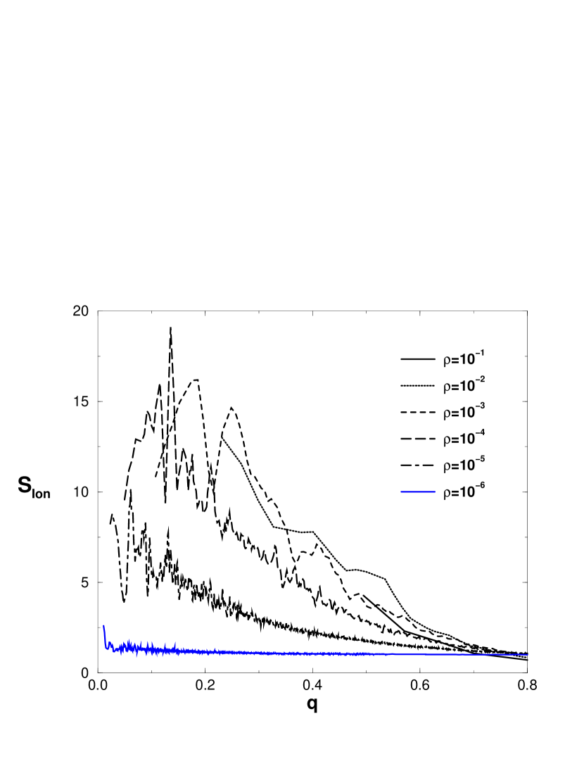
Figure 21: The structure factor $S_{ion}(q)$ vs. $q$ of the counter ion distribution for the indicated densities $\rho$. For lower densities the structure factor becomes similar to the one of a homogeneous background.

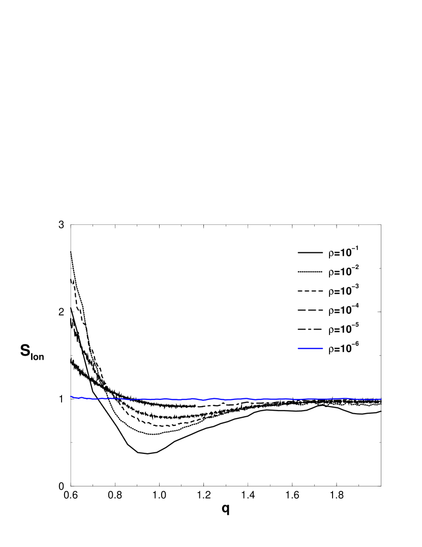
Figure 22: Blow up of Fig. 21 for large $q$. One can detect a minimum of the structure factor for $q\approx 1.0$, which is reminiscent of a correlation hole of the counterion cloud.

The determination of the fraction of bound (immobile) counterions is very difficult to accomplish experimentally. We imagine that particularly with x-ray and synchrotron scattering for some well prepared systems one could achieve a sufficient contrast between the counterions and the chains. As the majority of the chain atoms are carbon, hydrogen and oxygen the use of heavy counterions like cesium should give a sufficient contrast in scattering intensities. Therefore the structure factor of the counterion distribution should be measurable. This quantity is much easier calculated in the simulation, because the counterions are more mobile and outnumber the number of polymers by far. So their distribution in the system can be dissolved in much more detail. The simulations show very interesting results, as for example in Figure 21 where the density dependency of the small $q$ part of the counterion structure factor is shown. For high and medium densities the distribution is coupled to that of the polymers and shows a pronounced signal of the underlying structure. For the highest density, the structure factor shows no clear peak. This is the reflection of the relatively uniform distribution of the counterions in the microgel. In the medium density range a maximum shows up which increases and moves to smaller $q$-values with decreasing density. In the case of $\rho=2\cdot 10^{-5}\sigma^{-3}$ the intensity decreases, because more and more counterions leave the strongly stretched chains so that a significant background contributes to the scattering. For the lowest density only this background of uniformly distributed counterions remains, leading to a completely flat and unstructured scattering function. For higher $q$ a clear minimum is detected, which is getting deeper with decreasing density, as can be seen in Figure 22. Of course, the lowest density still gives the flat signal from the uniform background. This minimum can be interpreted as a correlation hole between the counterion clouds. At higher densities, many of the counterions are condensed and therefore near the chains. The number of free counterions is relatively small compared to the free volume between the chains which spans almost the whole volume of the solution, as can be seen in Figure 11. This concentration difference is reflected by the structure factor. At even higher $q$-values a second maximum can be detected for the higher densities in the simulation data. It is located around the $q$-value related to the radius of gyration of the polyelectrolytes reflecting the correlation of the chains within the counterion cloud around one monomer. As the amplitude is very small this effect is difficult to analyze quantitatively, however we consider it not to be relevant for experimental studies at present, and do not analyze it in further detail here.

6 Conclusions

We present a set of MD simulations studying the influence of a poor solvent on the structural properties of strongly charged, flexible polyelectrolyte chains in salt free solution.

We showed that the underlying neutral system is characterized by a $\theta$ point which we determined to be $\epsilon_{LJ,\theta}=0.34\pm 0.02$. In the beginning three different values of the strength of the hydrophobicity ($\epsilon_{LJ}=0.25$, 0.5, and 1.0) were examined at a polymer density of $\rho=10^{-4}\sigma^{-3}$. The value of $\epsilon_{LJ}=0.25$ lead to hydrophilic behavior as expected, because this value is even below the neutral $\theta$ point. However, the other two values of $\epsilon_{LJ}$ showed as well only a weak influence of the attractive interaction and the differences to the purely hydrophilic chains was rather small. By varying the Bjerrum length $\lambda_{B}$ however, we could demonstrate that under the right conditions weak hydrophobicities can nevertheless lead to strong effects. For $\epsilon_{LJ}=0.5$ the chains showed a stretching followed by a strong contraction with increasing Bjerrum length. This effect is well known from simulations of hydrophilic polyelectrolytes, but in our hydrophobic case it is more pronounced and shifted to smaller $\lambda_{B}$.

An “effective” $\theta$ point was calculated for the charged system for a density of $\rho=10^{-4}\sigma^{-3}$. The condition that its end-to-end distance equals the one for a ideal, neutral chain of the same length resulted in $\epsilon_{LJ,\theta_{eff}}^{(c)}=1.51\pm 0.03$. This value was taken as a starting point for detailed study of the chain conformations under a variation of the polymer density. At high densities we found a high screening of the electrostatic interactions, favoring the short range hydrophobic attraction, whereas at low densities the Coulomb forces clearly dominated. A multitude of chain conformations ranging from micro-gels via isolated, strongly collapsed chains to extremely stretched necklace chains was found. The collapsed objects showed locally Porod scattering ($S(q)\propto q^{-4}$), while the necklace like objects showed a logarithmic slope of their scaling function of $m=-1$ ($\nu=1$), so that both extremes are realized in one system that differs only by density. A micro-phase separation was not observed. We estimated from our simulation that an agglomeration of two chains is unfavorable for the density $\rho=2\cdot 10^{-2}\sigma^{-3}$, whereas more detailed estimates are given in [20]. To sum up, the polymer density seems to be a very useful parameter to vary to study polyelectrolytes under poor solvent conditions. The preparation of such systems should be extremely fruitful also for experiments, because the density $\rho$ can be very easily controlled. The comparison of the MD data of the structure factor of the monomer pair correlation with experimental data indicates that the knowledge of the real number of free charges in the system is of central importance in understanding the behavior of polyelectrolyte solutions, especially for the poor solvent case. Measurements of the counterion structure factor would be very helpful in comparison to the simulation results presented here.

We could relate the structural properties of polyelectrolytes under good and poor solvent conditions within one consistent approach. This gave a clear and conclusive picture of the influence of solvent quality on the structure of flexible polyelectrolyte chains.

• Molecular Dynamics

• Lennard-Jones

• finite extension nonlinear elastic

• Particle-Mesh-Ewald

• sulfonated polystyrene

• purely repulsive hydrophilic potential

• hydrophobic potential showing a short range attraction

• Finite Extension Nonlinear Elastic bond potential between chain monomers

• end-to-end distance

• radius of gyration

• characteristic ratio $r=\frac{R^{2}_{end}}{R_{G}}$

• Numbers of monomers of a chain

• linear length of the simulation cell

• average bond length

• Bjerrum length

• Debye-Hückel parameter

• unit charge

• valence of a unit charge

• fraction of charged monomers

• chemical charge density

• critical charge determined by the Rayleigh criterion

• Coulomb energy

• distance between globules

• Boltzmann constant

• Temperature

• Lennard-Jones length unit (monomer radius)

• Lennard-Jones time unit

• permittivity of the vacuum and the solvent, respectively

• friction coefficient of the Langevin dynamics

• time step of the velocity Verlet MD algorithm

• Manning Parameter

• critical Manning parameter

• density: number of monomers per simulation volume

• $\theta$ - temperature of the neutral system

• $\theta$ - temperature of the charged system

• LJ energy parameter giving the $\theta$ point of the neutral system

• LJ energy parameter giving the effective $\theta$ - point of the charged system

• reduced temperature to the critical $\theta$ - point

• sphericall averaged structure factor

• component of the spherically averaged structure factor along the first principal axis of inertia

• magnitude of the Fourier space vector

• position of the maximum of the structure factor

• osmotic pressure

• scaling exponent of the chain extension

• scaling exponent of the maximum of the structure factor

• charge concentration

• density of mobile, noncondensed counterions

Variation of the effective screening for hydrophobic polyelectrolytes
$\rho[\sigma^{-3}]$	$\text{N}_{C}$	$\text{N}_{ch}$	$\rho_{ch}[\sigma^{-3}]$	$\kappa^{-1}[\sigma]$	$y$
$2\cdot 10^{-1}$	25,5	208	$1.95\cdot 10^{-2}$	1.17
$2\cdot 10^{-2}$	26	192	$1.85\cdot 10^{-3}$	3.79	0.51
$2\cdot 10^{-3}$	24.5	240	$2.3\cdot 10^{-4}$	10.67	0.45
$2\cdot 10^{-4}$	21	352	$3.44\cdot 10^{-5}$	27.75	0.41
$2\cdot 10^{-5}$	13	608	$5.93\cdot 10^{-6}$	66.87	0.38
$2\cdot 10^{-6}$	3	928	$9.06\cdot 10^{-7}$	171	0.41

Table 1: Variation of the effective screening with density for hydrophobic polyelectrolytes. $N_{C}$ denotes the number of condensed counterions, $N_{ch}$ is the number of free charges, and $\rho_{ch}$ is the density of free charges. The exponent $y$ is obtained via $\kappa^{-1}\propto\rho^{y}$. One recognizes a deviation of $y=1/2$ due to counterion condensation

Variation of the effective screening for hydrophilic polyelectrolytes
$\rho[\sigma^{-3}]$	$\text{N}_{C}$	$\text{N}_{ch}$	$\rho_{ch}[\sigma^{-3}]$	$\kappa^{-1}[\sigma]$	$y$
$2\cdot 10^{-1}$	24	256	$2.4\cdot 10^{-2}$	1.05
$2\cdot 10^{-2}$	21	352	$3.4\cdot 10^{-3}$	2.79	0.42
$2\cdot 10^{-3}$	18	448	$4.3\cdot 10^{-4}$	7.85	0.45
$2\cdot 10^{-4}$	16	512	$5\cdot 10^{-5}$	23.03	0.47
$2\cdot 10^{-5}$	11.5	656	$6.4\cdot 10^{-6}$	64.38	0.45
$2\cdot 10^{-6}$	3	928	$9.06\cdot 10^{-7}$	171	0.42

Table 2: Variation of the effective screening with density for hydrophilic polyelectrolytes. The notation is the same as in Table 1. The variations are clearly much weaker than for the hydrophobic case.

Figure 1: Scaling analysis for determining the $\theta$ point of the neutral system. Plotted is $\epsilon_{LJ}^{-1}$ vs. $N^{-0.5}$ according to Eq. 7, where $T=\epsilon_{LJ}^{-1}$ in our units. One obtains straight lines $\text{N}^{-\frac{1}{2}}\rightarrow 0$ which converge up to corrections of higher order to the $\theta$ point. $\theta_{eff}$ describes the $\theta$ point for the finite chain, where $\epsilon_{LJ}$ was chosen such that its $R_{end}$ had the same value as an equally long random walk. These values converge as well to the $\theta$ point for $N\rightarrow\infty$. One obtains $\epsilon_{LJ,\theta}^{(n)}=\frac{1}{2.96\pm 0.06}=0.34\pm 0.02$.

Figure 2: Comparison of the spherically averaged structure factor, $S_{sp}(q)$ (top curve) and its component along the first principal axis of inertia, $S_{\parallel}(q)$ (bottom curve), versus $q$ for various hydrophobic interaction strengths $\epsilon_{LJ}=$ 0.25, 0.5, and 1.0 at a density $\rho=10^{-4}\sigma^{-3}$.

Figure 3: Comparison of the radius of gyration $R_{G}$ versus density $\rho$ of hydrophilic (phil) and weakly hydrophobic ($\epsilon_{LJ}=0.5$) polyelectrolytes.

Figure 6: Number of condensed counter ions $N_{C}$ as a function of the Bjerrum length $\lambda_{B}$ for $\epsilon_{LJ}=0.5$ at the density $\rho=2\cdot 10^{-3}\sigma^{-3}$. The number of counterions per chain is 32.

Figure 7: Spherically averaged structure factor $S_{sp}(q)$ vs. $q$ for various Bjerrum lengths $\lambda_{B}$ for hydrophobic chains with $\epsilon_{LJ}=0.5$.

Figure 9: Bond length $b$ versus density $\rho$ for hydrophilic (phil), weakly hydrophobic ($\epsilon_{LJ}=0.5$), and hydrophobic ($\epsilon_{LJ}=1.5$) polyelectrolyte chains.

Figure 10: Density dependence of the end-to-end distance $R_{end}$ (top) and the statistical ratio $r$ (bottom) vs. density $\rho$ for hydrophilic (phil), weakly hydrophobic ($\epsilon_{LJ}=0.5$), and strongly hydrophobic ($\epsilon_{LJ}=1.5$) systems.

Figure 12: A snapshot of the whole simulation box, showing 16 chains together with their counterions for the density $\rho=2\cdot 10^{-1}\sigma^{-3}$. The beads are the charged monomers, the counterions are indicated as small black spheres, and the neutral monomers are dark grey spheres.

Figure 13: A typical poor solvent polyelectrolyte conformation for the density $\rho=2\cdot 10^{-1}\sigma^{-3}$. The coloring is the same as in Fig.11

Figure 14: Details of the spherically averaged structure factor $S_{sp}(q)$ for large $q$ for the indicated densities $\rho$. The straight lines have slope $m=-2,-3$, and $-4$, respectively.

Figure 15: The number $N_{c}$ of condensed counter ions per chain as a function of density $\rho$ for $32$ charged monomers per chain for hydrophilic chains (phil) and hydrophobic chains with $\epsilon_{LJ}=0.5$ and 1.5.

Figure 16: Details of the spherically averaged structure factor $S_{sp}(q)$ vs. $q$ for small $q$, obtained for the indicated densities $\rho$. The straight lines have all slope $m=-1$, and the vertical lines denote the value of $q=2\pi/R_{G}$.

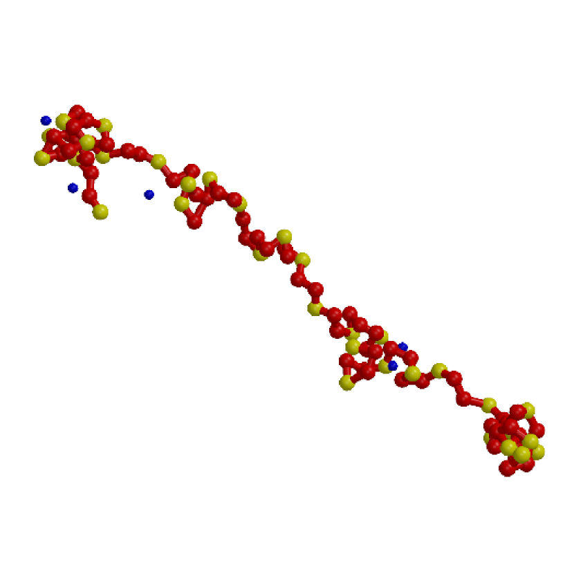
Figure 18: A typical poor solvent polyelectrolyte conformation for the density $\rho=2\cdot 10^{-6}\sigma^{-3}$, showing a very elongated, but still visible pearl-necklace structure. The coloring is as in Fig. 11

References

-
[1]
P. J. Flory, Principles in Polymer Chemistry, Cornell University
Press,
Ithaca (1953). - [2] P. de Gennes, Scaling Concepts in Polymer Physics, Cornell University Press, Ithaca, NY (1979).
- [3] M. Doi and S. F. Edwards, The Theory of Polymer Dynamics, Oxford University Press, Oxford, NY (1986).
- [4] J.-L. Barrat and J.-F. Joanny, Adv. Chem. Phys. 94, 1 (1995).
- [5] T. B. Liverpool, M. Stapper, Europhysics Letters, 40, 485 (1997), and references therein.
- [6] U. Micka and K. Kremer, Phys. Rev. E 54 (3), 2653 (1996).
- [7] M. Stevens and K. Kremer, J. Chem. Phys. 103 (4), 1669 (1995).
- [8] M. Stevens and K. Kremer, Phys. Rev. Lett. 71, 2228 (1993); M. Stevens and K. Kremer, Macromolecules 26, 4717 (1993).
- [9] U. Micka and K. Kremer, J. Phys.: Cond. Matter 8, 9463 (1996); U. Micka and K. Kremer, Euro. Phys. Lett. 38 (4), 279 (1997).
- [10] J.-L. Barrat and J.-F. Joanny, Europhys. Lett. 24, 333 (1993).
- [11] C. E. Woodward, B. Jönsson, Chem. Phys. 155, 207 (1991)
- [12] S. Förster and M. Schmidt, Adv. Poly. Sci. 120, Springer Verlag Berlin, Heidelberg (1995).
- [13] A. V. Dobrynin, M. Rubinstein and S. P. Obukhov, Macromolecules 29, 2974 (1996).
- [14] Lord Rayleigh, Philos. Mag. 14, 184 (1882).
- [15] W. Essafi, Ph. D. thesis, Universit t VI, Paris (1996), unpublished.
- [16] W. Essafi, F. Lafuma, C. E. Williams, J. Phys. II 5, 1269 (1995).
- [17] A. Lyulin, B. Dünweg, O. Borisov, A. Dariinski, preprint, and Burkhard Dünweg, private communication.
- [18] H. Morawetz, Macromolecules 31, 5170 (1998).
- [19] A. R. Khokhlov and K. A. Katchaturian, Polymer 23, 1742 (1982).
- [20] U. Micka, K. Kremer, Phys. Rev. Lett. submitted.
- [21] P. P. Ewald, Ann. Phys. 64, 253 (1921); S. W. de Leeuw, J. W. Perram and E. R. Smith, Proc. R. Soc. Lond. A 373, 27 and 57 (1980).
- [22] T. A. Darden, D. M. York and L. G. Pedersen, J. Chem. Phys. 98 (12), 10089 (1993).
- [23] H. G. Petersen, J. Chem. Phys. 103 (9), 3668 (1995).
- [24] M. Deserno, C. Holm, J. Chem. Phys.109, 7678 (1998); J. Chem. Phys. 109, 7694 (1998).
- [25] G. S. Grest and M. Murat, Macromolecules 26 (2), 3108 (1993).
- [26] J. Batoulis and K. Kremer, Euro. Phys. Lett. 7(8), 683 (1988).
- [27] G. S. Manning, J. Chem. Phys. 51, 924, 934 & 3249 (1969); Q. Rev. Biophys. 11, 179 (1981).
- [28] C. F. Anderson and J. M. Recor, Annu. Rev. Phys. Chem. 33, 191 (1982).
- [29] F. Oosawa, Polyelectrolytes, Marcel Dekker, New York (1971).
- [30] private communication to G. S. Manning (see Reference 13 in G. S. Manning, J. Chem. Phys. 51, 924 (1969)).
- [31] R. G. Winkler, M. Gold, P. Reineker, Phys. Rev. Lett. 80, 3731 (1998).
- [32] G. Porod, Kolloid. Z. 124, 83 (1951).
- [33] M.-N. Spiteri, Ph.D. thesis, Université Paris IV (1997), unpublished.
- [34] U. Micka, Ph.D. thesis, Universität Bonn (1997), published as Jül-3451 by the Forschungszentrum J”ulich.
List of Abbrevations and Symbols
-
MD