Dissipative properties of vibrated granular materials

Abstract

We investigate collective dissipative properties of vibrated granular materials by means of molecular dynamics simulations. Rates of energy losses indicate three different regimes or “phases” in the amplitude-frequency plane of the external forcing, namely, solid, convective, and gas-like regimes. The behavior of effective damping decrement in the solid regime is glassy. Practical applications are dicussed.

PACS: 05.40. -y, 46.10 +z, 83.70 Fn.

The dominating approach in the world of vibration control and suppression by granular systems has been mainly practical [1]. Granular motion relaxes rapidly once the energy supply is switched off, and dampers can efficiently absorb energy released by shocks of external forcing. Engineers classify granular dampers as passive ones.

For the case of “granular gases”, i.e. particulate systems in a state where the mean free path is large as compared with particle sizes the cooling rate, the dissipation rate of the system has been investigated [2], and applications of this work require an analysis of granular gas (hydro)dynamics in a given experimental setup. Damping in dense granular arrangements is a much more difficult problem which is mostly studied experimentally.

In this work, by using molecular dynamics simulations, we show that granular systems reveal different damping regimes indicating collective dissipation modes. Our study of these regimes leads to a “phase diagram” of horizontally vibrated granular systems (see Fig. 4). By using this diagram along with the presented estimates for damping decrements, practitioners may accelerate the design and testing procedures.

In simulations we focus on two dimensional containers which are partially filled with granular material and shaken horizontally. The motion of the container is sinusoidal, $x(t)=A\sin(\omega t)$; it mimics practical situations where dampers are tested in the vicinity of the eigenmodes of the vibrating mechanism. We study the reaction of the system to the choice of parameters of shaking $A$ and $\omega$, keeping all other parameters (size, roughness and hardness of particles, filling factor, size and shape of the apparatus) fixed [3].

Our primary objective is the rate of energy dissipation, computed by cycle averaging under steady conditions of oscillatory motion. Dissipation is obtained by using two different ways to ensure consistency of the data: (i) from the total power transmitted to the container walls, and (ii) from the dissipative work in inter-particle collisions. Numerically, both results coincide within a few percent.

For the molecular dynamics simulations, we use a modified soft-particle model by Cundall and Strack [4]: Two particles $i$ and $j$, with radii $R_{i}$ and $R_{j}$ and position vectors $\vec{r}_{i}$ and $\vec{r}_{j}$, interact if their compression $\xi_{ij}=R_{i}+R_{j}-\left|\vec{r}_{i}-\vec{r}_{j}\right|$ is positive. In this case the colliding spheres feel forces $F_{ij}^{N}$ [5] and $F_{ij}^{S}$ [6], in normal and shear directions denoted by unit vectors $\vec{n}^{N}$ and $\vec{n}^{S}$, respectively,

$$F_{ij}^{N}=\left(Y\sqrt{R^{\,\mbox{\it\it eff}}_{ij}}\right)/\left(1-\nu^{2}\right)~{}\left(\frac{2}{3}\xi^{3/2}+a\sqrt{\xi}\,\dot{\xi}\right)$$ (1)

$$F_{ij}^{S}=\mbox{sign}\left({v}_{ij}^{\,\mbox{\it\it rel}}\right)\min\left\{\gamma_{S}m_{ij}^{\,\mbox{\it\it eff}}\left|{v}_{ij}^{\,\mbox{\it\it rel}}\right|~{},~{}\mu\left|F_{ij}^{N}\right|\right\}$$ (2)

and the resulting momenta acting upon the particles are $M_{i}=F_{ij}^{S}R_{i}$, $M_{j}=-F_{ij}^{S}R_{j}$. The constant $a$ is the characteristic dissipation rate of the material, $Y$ is the Young modulus and $\nu$ the Poisson ratio. The normal and shear friction coefficients, $\gamma_{n}\equiv aY/(1-\nu^{2})$ and $\gamma_{S}$, model dissipation during particle contact. Eq. (2) takes into account that the particles slide upon each other for the case that the Coulomb condition $\mu\!\left|F_{ij}^{N}\right|<\left|F_{ij}^{S}\right|$ holds, otherwise they feel some viscous friction. $R^{\,\mbox{\it\it eff}}_{ij}=R_{i}R_{j}/\left(R_{i}+R_{j}\right)$ is the effective radius, and the effective mass $m_{ij}^{\,\mbox{\it\it eff}}$ is defined analogously. The relative velocity at the point of contact is

$${v}_{ij}^{\,\mbox{\it\it rel}}=(\dot{\vec{r}}_{i}-\dot{\vec{r}}_{j})\cdot\vec{n}^{S}+R_{i}{\Omega}_{i}+R_{j}{\Omega}_{j}\;,$$ (3)

with $\Omega_{i}$ and $\Omega_{j}$ being the angular velocities of the particles.

The values of the coefficients used in simulations are $Y/(1-\nu^{2})=7.5\times 10^{7}$, $\gamma_{n}=7\times 10^{2}$, $\gamma_{S}=30$, $\mu=0.5$. Cgs units are implied throughout the paper.

With the system parameters specified above, depending on forcing one may find intensive convection (Fig. 1). Convection patterns in horizontally vibrated granular material have been recently reported [7]. In our case only two rolls could be observed. Different aspect ratios or material parameters give different convection patterns, with 2, 4[7] or more convection rolls (not shown here)[8].

  

 

FIG. 1.: Images of the cycle-averaged motion of the system vibrated at $f=20$ for different velocities of forcing, $A\omega$: a) 1900, b) 1250, c) 600, d) 100, e) 15.

The velocity profiles in Fig. 1 have been produced by averaging particle velocities in the regime of steady oscillations. We do not intend to discuss the effect of convection in horizontally shaken material in detail, although we note that the onset of convection in the system is due to a critical amplitude of driving velocity $\left(A\omega\right)_{cr}$. Fig. 2 shows the maximum absolute value of convective motion in the system, i.e. the length of the longest arrow in Fig. 1, over the velocity amplitude $A\omega$ for different frequencies $f$ (in Hz). Below $\left(A\omega\right)_{cr}\approx 60$ there is slow collective motion in the system, but close to this point there is a transition into a rapid convective regime (see also Fig. 1d).

To characterize the dissipation in the system we introduce an effective damping parameter $b$ which is proportional to the ratio between the averaged dissipated power per cycle $T$ and the mean translational kinetic energy of the granular system [9],

$$b=\frac{\frac{1}{T}\int_{T}W_{\mbox{\em diss}}(t)dt}{2\sum_{n}m_{n}\int_{T}v_{n}^{2}(t)dt}\,.$$ (4)

Here summation is performed over all granular particles in the container. In the reference case of linear oscillator the damping decrement $b$ equals the inverse of the amplitude relaxation time.

FIG. 2.: Maximum velocity of collective flow $V$ over amplitude of shaking velocity $A\omega$, for the different frequencies analyzed: $\diamond:5$; $\Box:10$; $\circ:20$; $\triangleright:40$; $\triangle:80$ (Hz).

Fig. 3 shows the damping $b$ as a function of the effective acceleration $\Gamma=A\omega^{2}/g$ and the amplitude of the velocity of vibration, $A\omega$. Different symbols (filled or open) display different frequencies. Except for the very low frequency range, $b$ scales with the amplitude of the velocity of vibration, $A\omega$ (Fig. 3a). A transition from the $A\omega$-scaling into another regime takes place at $\Gamma\approx 1$ (Fig. 3b). Below this point the effective damping parameter becomes less sensitive to $\Gamma$ and fluctuates very strongly.

FIG. 3.: Effective damping parameter $b$ vs the amplitude of velocity of vibration, $A\omega$ (a); vs the dimensionless forcing acceleration parameter, $\Gamma$ (b). Different symbols refer to different frequencies; $\triangleleft:2.5$; $\diamond:5$; $\Box:10$; $\circ:20$; $\triangleright:40$; $\triangle:80$ (Hz). Open symbols refer to fast cooling schedule, filled symbols refer to slow cooling (see text for details). The solid line in (a) shows a fit using (6) and (7). Observe the fit lines with slopes -1 and +1 for $b\propto(A\omega)^{-1}$ and $b\propto(A\omega)^{+1}$in the “liquid” and “gas” regimes, resp.

Fig. 3 reveals three regions, indicative of different dynamic regimes. The local minimum in Fig. 3a is the region of spatially organized behavior with well developed convection rolls, where the entire granular mass participates in collective motion (Fig. 1c). For higher velocity amplitudes $A\omega$, the dissipation rate increases, as particles begin to fly across the box and the ordered structure of the rolls starts to disappear (cf. Fig. 1a-b). The minimum corresponds to a characteristic velocity at which the system begins to display the “gas” state. This characteristic velocity can be estimated by equating the characteristic time of motion in horizontal and vertical directions for a particle with velocity of the order of $A\omega$,

$$L/A\omega=A\omega/g\,.$$ (5)

For $L=100$, this gives $A\omega=313$, which gives an order-of-magnitude estimate of the minimum of Fig. 3a. Additional analysis reveals that the correct prefactor is close to 2 (see Fig. 4a and discussion below). At higher velocities particles continue to stay airborne, and gravity becomes unimportant. Thus, the boundary $A\omega\sim\sqrt{Lg}$ separates the “liquid” and gas-like regimes [10].

To the left from the minimum, with amplitude decrease at any frequency, the depth of the rolls diminishes progressively until a critical value $(A\omega)_{cr}\approx 60$ is reached. At this velocity the rolls vanish completely and we do not find organized motion in the system anymore (cf. Figs. 2 and 1d). The system seems to be in a “solid” state. The critical value of velocity is manifested in Fig. 3a by a change in the damping slope. Given that the acceleration of shaking here exceeds $g$, critical velocity in this range points to $A\omega\sim\sqrt{Rg}$, where $R$ is the particle radius. This is consistent with our particle sizes [3].

In the solid regime one has to switch from velocities to accelerations. Following Fig. 3b to small accelerations, one finds a change in the behavior at $\Gamma\approx 1$, i.e. when the maximal acceleration of shaking becomes comparable with gravity $g$. For $\Gamma\gtrsim 1$ the curves are smooth, but for $\Gamma\lesssim 1$ suddenly the data become very noisy. At this point the grains form a glassy “solid” phase. We note that our understanding of the transition at $\Gamma\lesssim 1$ is different from the solid-fluid transition reported recently [11] as long as $A\omega\lesssim\sqrt{Rg}$. At higher velocities our results lead to the same conclusions as the results reported in Ref. [11].

To reiterate, the transition point found in Ref. [11] is given by $A\omega^{2}=g$ in our notation. It is unclear whether the non-glassy solid phase at $\Gamma\gtrsim 1$ can be identified by the method of granular temperature used in Ref. [11]. If our understanding is correct, the non-glassy regime is not necessarily fluidized, and the region of increasing granular temperature may overlap the region of non-vanishing configurational order associated with a “solid” state. This is an intriguing issue, and it is worth a separate study.

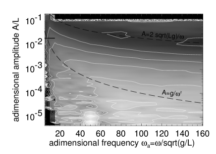
FIG. 4.: Phase diagram of our system, and the damping regimes. (a): explicitly analyzed regions, the value of the damping parameter $b$ shown by grey scale vs the adimensional frequency and amplitude of shaking (white - highest damping). “Mountains” at low amplitudes are caused by fluctuations in the glassy state. The black stripe at the very top of the picture represents empty data and should not be taken into account. The diagram (b) is a summary of regimes based on the entire analysis. The narrow region between the glass state and dashed line is found to be a non-glassy “solid”.

At the glass transition point, $\Gamma\approx 1$, particle ensembles get trapped in their momentary position. In the glassy regime the rate of dissipated energy is strongly sensitive to the configurational arrangement of the particles i.e. to the history of the system. In other words, depending on initial conditions, for the same parameters of oscillation $A$ and $\omega$, the system can settle in different configurational arrangements, and exhibit different dissipation rates. Transitions between different condensed phases based on multi-particle condensation have been suggested earlier by two of the authors [2].

To demonstrate this fact, in Fig. 3a two different sets of data points are shown by filled and open symbols; they refer to “fast” and “slow” cooling. By fast cooling we mean an instantaneous transition from any fluidized initial state to the specified amplitude and frequency of vibration. The initial conditions, namely, random positions and velocities of particles, are kept the same for each data point. Thus, there is no memory of the preceding evolution. Having the first 30 cycles of the driving oscillation discarded, the mean dissipation is obtained by averaging over 30 cycles of shaking. The large fluctuation of the dissipation rate $b$ is not due to insufficient data averaging: averaging over 100 cycles, instead of 30, leads to the same results. In the case of slow cooling, the system is initialized only once for each frequency, and the final state for a certain amplitude $A$ serves as the initial one for the next amplitude to be investigated. The amplitude of vibration in each simulation is diminished by a factor of 1.2. The behavior in this case can be sensitive to the entire history of the experiment. According to the mechanism discussed in Fig. 3a, in the region $\Gamma\lesssim 1$ the fast cooling data points begin to fluctuate, whereas the slow cooling data are relatively smooth. Thus, for accelerations $\Gamma\lesssim 1$ one identifies a glass regime.

The different damping regimes can be clearly appreciated in Fig. 4a, where a shaded contour plot of the effective damping parameter is shown as a function of the adimensional amplitude and frequency of shaking [10]. These results suggest that, on the $(A,\omega)$ plane, the regime boundaries form a diagram similar to the Van der Waals system, with the “triple point” roughly located at $(L,\sqrt{g/L})$. Above this point, direct “sublimation” is achieved at $A\omega^{2}\approx g$. Convection rolls can develop at $A<L$ above a critical velocity, as has been discussed. This diagram is shown schematically in Fig. 4b, where for the seek of clarity the boundaries between regimes are sharpened. The damping decrement along with convection dynamics provide indicative suggestions about “phases” which we discuss here. Any sound indentification of transitions and phases can only be based on studies of appropriate order parameters. In principle, it is conceivable that some “phases” may represent only preferred dynamic states.

The fluidized regime is amendable to hydrodynamical arguments. Let us consider the “gas” state, where the dissipation is dominated by collisions with the walls of the container. The pressure transmitted to the vertical wall by the granular cloud of density $\rho$ which moves with velocity $v=A\omega$ relative to the wall is $\sim\rho A^{2}\omega^{2}$. Neglecting other contributions, the dissipated power during the collision is then roughly a fraction of the quantity $\rho v^{3}L$. Using Eq. (4) one finds

$$b=C_{g}\frac{A\omega}{L}\,.$$ (6)

Formula (6) is applicable at $A\omega\gtrsim\sqrt{Lg}$. $C_{g}$ is some unknown numerical prefactor. This expression is simply proportional to the collision frequency of independent gas particles moving at velocity $A\omega$ and having a mean free path of the order of $L$. In other words, collective modes are irrelevant in the “gas” phase as it should be.

For velocities $A\omega<\sqrt{Lg}$, the system is only partially fluidized. This means that the pressure transmitted by the container walls does not exceed the static stress that the condensed particles can sustain. The latter is roughly of the order of $p=\rho gL$ in horizontal direction. As long as there is any fluidized material in the system, these stresses cannot be lower. Therefore, the dissipated power is $pHv$, where $H$ is the height of the system. Dividing it by the total kinetic energy $\frac{1}{2}\rho HLv^{2}$ one gets

$$b=C_{l}\frac{g}{A\omega}\,.$$ (7)

Formula (7) is applicable at $A\omega^{2}\gtrsim g$, $A\omega\gtrsim\sqrt{Rg}$, $A\omega\lesssim\sqrt{Lg}$, and $C_{l}$ is the unknown numerical prefactor. Very roughly, in this regime some condensed particles transmit their motion to other particles and the latter can move against gravity. $b$ is the inverse time needed to decelerate them. The best fit of the curves of Fig. 3 provides the values $C_{g}=0.1$ and $C_{l}=0.45$ for our simulated system, giving a value for the minimum $(A\omega)_{G}=2.1\sqrt{Lg}$. This is obviously consistent with the upper curve shown in Fig. 4a, separating the “fluid” and “gas” regimes.

To summarize, by means of MD simulations we have shown how the analysis of energy-loss rate displays different damping regimes. In particular, one finds that fully convective states correspond to minimal damping decrement. Performing two types of measurements, referred as to slow and fast cooling, one identifies a glass regime. This regime, in which configurational states affect the dynamical properties of the system, is separated from the fluidized regime by the value of the forcing parameter, $\Gamma\equiv A\omega^{2}/g\sim 1$. For higher forcing one may find a non-glassy solid phase as long as the velocity of shaking is smaller than $A\omega\lesssim\sqrt{Rg}$. The $A\omega$-scaling of the damping curves signals the beginning of the “fluid” regime. Here convective states can develop in a region of the plane $(\omega,A)$ above the critical velocity $A\omega\sim\sqrt{Rg}$, critical acceleration $A\omega^{2}/g\gtrsim 1$ and below “evaporation” threshold $A=\sqrt{Lg}/\omega$. The damping decrement passes through the minimum for velocities $A\omega\sim\sqrt{Lg}$, and at higher velocities a gas-like state can be identified, where the effects of gravity are negligible.

The authors thank V. Buchholtz for discussions. Invaluable help and encouragement by S. Simonian and multiple discussions of practical issues are gratefully acknowledged. The calculations have been done on the parallel computer KATJA (http://summa.physik.hu-berlin.de/KATJA/) of the medical department Charité at the Humboldt University in Berlin. The work was supported in part by Deutsche Forschungsgemeinschaft through Po 472/3-2.

REFERENCES

- [1] C. Grubin, ASME Journal of Applied Mechanics 23, 373 (1956); A. Papalou and S. F. Masri, ASME J. Vibr. Acoust. 118, 614 (1996); H. V. Panossian, ASME J. Vibr. Acoust. 114, 101 (1992); S. S. Simonian, Proceedings SPIE 2445 149, (1995).
- [2] I. Goldhirsch and G. Zanetti, Phys. Rev. Lett. 70, 1619 (1993); S. McNamara and W. R. Young, Phys. Rev. E 50 R28 (1993); S. E. Esipov and T. Pöschel, J. Stat. Phys. 86, 1385 (1997); T. Schwager and T. Pöschel, Phys. Rev. E 57, 650 (1998); K. Shida, T. Kawai, Physica A 162, 145 (1989).
- [3] We use 500 circular particles with radii homogeneously distributed in and density , placed in a square container of side . The filling fraction is 20%. The rough inner walls of the container are simulated by attaching additional particles of the same material properties, technique which is similar to “real” experiments, e.g. E. E. Ehrichs et al. Science 267, 1632 (1995).
- [4] P. A. Cundall and O. D. L. Strack, Géotechnique 29, 47 (1979).
- [5] G. Kuwabara and K. Kono, Jpn. J. Appl. Phys. 26, 1230 (1987); N. V. Brilliantov, F. Spahn, J.-M. Hertzsch, and T. Pöschel, Phys. Rev. E, 53, 5382 (1996); W. A. M. Morgado and I. Oppenheim, Phys. Rev. E 55, 1940 (1997).
- [6] P. K. Haff and B. T. Werner, Powder Technol. 48, 239 (1986).
- [7] K. Liffman, G. Metcalfe, P. Cleary, Phys. Rev. Lett. 79, 4574 (1997); K. Liffman and G. Metcalfe, In: R. P. Behringer and J. T. Jenkins, Powders and Grains ’97, p. 405, Balkema (Rotterdam, 1997); C. Salueña, S. E. Esipov, and T. Pöschel, ibid p. 341.
- [8] Many examples and related research can be found in http://summa.physik.hu-berlin.de/~kies.
- [9] The rotational energy has not been taken into account in the denominator of (4) because the rotational energy represents a small fraction of the translational kinetic energy (less than 5%).
- [10] Note that the existence of the -dependent transition point along with system-independent threshold , makes it necessary to perform a proper scaling of amplitudes (by ), frequencies (by ) and velocities (by ) in order to compare results for different container lengths in the shaking direction.
- [11] G. H. Ristow, G. Straßburger, I. Rehberg, Phys. Rev. Lett. 79 5, 833 (1997).