Quantum kinetics and thermalization in a particle bath model

Abstract

We study the dynamics of relaxation and thermalization in an exactly solvable model of a particle interacting with an harmonic oscillator bath. Our goal is to understand the effects of non-Markovian processes on the relaxational dynamics and to compare the exact evolution of the distribution function with approximate Markovian and Non-Markovian quantum kinetics. There are two different cases that are studied in detail: i) a quasiparticle (resonance) when the renormalized frequency of the particle is above the frequency threshold of the bath and ii) a stable renormalized ‘particle’ state below this threshold. The time evolution of the occupation number for the particle is evaluated exactly using different approaches that yield to complementary insights. The exact solution allows us to investigate the concept of the formation time of a quasiparticle and to study the difference between the relaxation of the distribution of bare particles and that of quasiparticles. For the case of quasiparticles, the exact occupation number asymptotically tends to a statistical equilibrium distribution that differs from a simple Bose-Einstein form as a result of off-shell processes whereas in the stable particle case, the distribution of particles does not thermalize with the bath. We derive a non-Markovian quantum kinetic equation which resums the perturbative series and includes off-shell effects. A Markovian approximation that includes off-shell contributions and the usual Boltzmann equation (energy conserving) are obtained from the quantum kinetic equation in the limit of wide separation of time scales upon different coarse-graining assumptions. The relaxational dynamics predicted by the non-Markovian, Markovian and Boltzmann approximations are compared to the exact result. The Boltzmann approach is seen to fail in the case of wide resonances and when threshold and renormalization effects are important.

I Introduction and Motivation

Recent advances in semiconductor femtosecond spectroscopy[1, 2] highlight the need for a deeper theoretical understanding of the relaxational dynamics of hot carriers that goes beyond Boltzmann kinetics. Boltzmann or semiconductor Bloch equations, are based on strict energy conservation and result in a Markovian description as a consequence of averaging over microscopic time scales. On short time scales, the time-energy uncertainty principle comes into play and off-shell (non-energy conserving) processes lead to quantum kinetic equations with memory effects, i.e. non-Markovian effects.

Ultrafast relaxation in semiconductors are typically studied by exciting a semiconductor sample with a femtosecond laser[3]-[5]. The subsequent dynamics of the photoexcited carriers is then studied by measuring the optical or transport properties of the sample at different time delays. These experiments demonstrate the breakdown of Boltzmann kinetics for periods less than the optical lattice oscillation period (around 115 fs in GaAs[5]) and emphasize the need for a quantum kinetic description of the relaxational dynamics.

Motivated by these new developments, there is a rekindled interest on a deeper theoretical understanding of quantum kinetics and critical analysis of transport and kinetic approaches are beginning to emerge[8]-[24]. In particular recently the initial stages of pre-equilibration during which quasiparticle correlations begin to build had been investigated in a many body system[8]. The pre-equilibrium stage cannot be studied within a Boltzmann approach because the early time dynamics depends on the initial preparation of the state and is determined by virtual processes that do not conserve energy on short times (off-shell).

Besides semiconductor systems, the interest in quantum kinetics is truly interdisciplinary: in dense plasma[9], nuclear matter[8, 10, 11] and high energy physics and cosmology[12]-[14] to cite but a few applications.

A very powerful method to derive quantum kinetic equations uses the non-equilibrium Green’s functions within the Keldysh formalism[15] which leads to the Kadanoff-Baym equations[16]. In order to derive quantum kinetic equations some assumptions must be invoked. Usually the generalized Kadanoff-Baym ansatz[17]-[21] with renormalized one particle Green’s function propagators[22] is used to relate the two-time correlation functions with the one-time distribution function. An alternative approach to derive quantum kinetic equations is by truncating the Bogolyubov-Born-Green-Kirkwood-Yvon (BBGKY) hierarchy[23, 24].

Although there is ample experimental and numerical confirmation of kinetics described by Boltzmann or kinetic Bloch equations in processes in which there is a wide separation between relaxational and microscopic time scales, the situation for non-Markovian quantum kinetics is less well understood.

An important limitation in the numerical study of non-Markovian kinetic equations is the very intensive computational requirements to analyze integro-differential equations with memory[25]. Thus it is important to try to test relaxation via non-Markovian quantum kinetic equations in systems which afford an exact solution. Recently non-Markovian quantum kinetics has been studied within the context of hot electron relaxation[21] in one dimension. This model affords an exact solution via bosonization and allows a direct comparison to an approximate kinetic treatment. Furthermore, improved transport equations that include the effects of correlations leading to a non-Markovian description have been recently proposed[24] and compared to available exact solutions in low dimensional models.

Thus the current experimental efforts in femtosecond relaxation in semiconductors and the necessity for a deeper understanding of quantum kinetics via non-Markovian transport equations justifies the study of model systems that can be solved exactly and thus provide a testing ground for the different types of approximations.

The goal of this article is to study the description of thermalization and relaxational dynamics in a simple and exactly solvable many body theory to obtain a deeper understanding of the off-shell processes (not energy conserving on short time scales) involved in thermalization and to provide a yardstick to test different approximations.

The aspects that we seek to study in this article are the following:

• How do off-shell effects modify the dynamics of thermalization and relaxation? By off-shell we here refer to processes that do not conserve energy on short time scales and threshold effects that are not incorporated in the usual Boltzmann equation. These are responsible for quasiparticle properties such as widths and wave function renormalization.

• A detailed understanding of the relaxation of quasiparticles vs. that of bare and dressed particles and to explore the definition of a quasiparticle distribution function that is valid beyond the narrow width approximation. The model under consideration also allows us to study the formation time of the quasiparticle.

• A comparison of the validity of Markovian (coarse grained) approximations including the Boltzmann equation, to a non-Markovian description of relaxation which is a simplified form of the Kadanoff-Baym equations.

Although we anticipate that the answer to many of these questions will in general depend on the details of the microscopic model, we propose to study a model of a particle (harmonic oscillator) interacting linearly with a bath of harmonic oscillators. As it will be seen in what follows this model bears many of the properties of more realistic interacting systems. By studying different couplings between the particle and the bath, we provide answers to these (and other) questions and obtain further intuition into more complex situations.

In section II we introduce the model and discuss the different approaches to study the dynamical evolution of the distribution function. In section III we analyze the dynamics from the point of view of the time evolution of an initially prepared density matrix which allows us to establish contact with the fluctuation dissipation relation. Here we distinguish between bare particle and dressed particle and quasi-particle distributions. The exact solution of the Heisenberg equations of motion is presented in section IV. In section V we study in detail the long time dynamics of the distribution function. In section VI we discuss the exact solution in terms of normal modes and analyze the definition of the quasiparticle number operator that describes the relaxational dynamics. In section VII we analyze the approximate relaxational dynamics in terms of i) the Boltzmann equation, ii) the non-Markovian quantum kinetic equation and iii) a Markovian approximation to the quantum kinetic equation. We provide a numerical comparison of the exact and approximate kinetics in section VIII. Our conclusions are summarized in section IX.

II The Model

As stated in the introduction, we seek to study aspects of quantum kinetics in a model that allows to compare approximate treatments of the relaxational dynamics to exact solutions. The model that we choose to describe this situation is that of an oscillator of bare frequency $\omega_{0}$ (representing the physical mass of the in particle states before the interaction) coupled linearly with a bath with an infinite number of degrees of freedom given by harmonic oscillators with frequencies $\omega_{k}$. Although this is a drastic simplification of microscopic interacting theories, this model continues to serve as a testing ground for studies of dissipation in quantum systems[26]-[32].

The Lagrangian is given by

$$L[q,Q_{k}]\,=\,\frac{1}{2}\left(\dot{q}^{2}\,-\,\omega_{0}^{2}q^{2}\right)\,+\,\frac{1}{2}\sum_{k}\left(\dot{Q}_{k}^{2}\,-\,\omega_{k}^{2}~{}Q_{k}^{2}\right)\,-\,q\sum_{k}C_{k}~{}Q_{k},$$

where the different coefficients of $\dot{q}^{2};~{}\dot{Q}^{2}_{k}$ (oscillator masses) had been absorbed by a canonical transformation into a redefinition of the couplings $C_{k}$. We now refer to the oscillator $q$ as the ‘system’ i.e. the degree of freedom whose dynamics we are interested in studying, and the oscillators $Q_{k}$ as the ‘bath’, these will be integrated out in the non-equilibrium effective action. This model also describes the interaction of an electron with a phonon or photon bath in the dipole approximation[31, 32].

We will eventually take the limit in which the bath oscillators are distributed continuously by introducing the bath spectral density $J(\omega)$ and where appropriate replacing the discrete distribution with a continuum one in the following manner:

$$J(\omega)=\frac{\pi}{2}\sum_{k}\frac{C^{2}_{k}}{\omega_{k}}~{}\delta(\omega-\omega_{k})$$

in such a way that

$$\sum_{k}C^{2}_{k}~{}f(\omega_{k})\rightarrow\frac{2}{\pi}\;\int d\omega\;\omega\;J(\omega)~{}f(\omega).$$ (1)

Our main goal is to study the evolution of the number of excitations or ‘particle distribution’ associated with the quanta of the system. Anticipating self-energy renormalization effects by the bath, we define a reference frequency $\Omega$ and introduce the operator that counts the number of quanta of the system’s degrees of freedom associated with this frequency

$$\hat{n}(t)\,=\,\frac{1}{2\Omega}\left[p^{2}(t)\,+\,{\Omega}^{2}q^{2}(t)\right]\,-\,\frac{1}{2}\;,$$ (2)

where $p(t)$ is the momentum of the particle. The reference frequency could either be taken to be the bare frequency $\omega_{0}$, or the frequency renormalized by the interaction with the bath, we will leave this choice unspecified for the moment.

Since the theory is quadratic we can resort to a number of different ways to study the dynamical evolution:

1. Given an initial density matrix we can evolve it in time exactly and obtain all of the non-equilibrium correlation functions.

2. The Heisenberg equations of motion for the operators can be solved exactly and again we can obtain any correlation function.

3. The normal modes can be found exactly, from which we can find the exact ground state and also obtain the operators that create the particle or quasiparticle states to study the asymptotic evolution of non-equilibrium states.

4. We compute exactly the expectation value of the proposed number operator in the canonical ensemble of the system plus bath and compare the result to the asymptotic form of the non-equilibrium distribution function. This allows an unequivocal description of thermalization in terms of the density matrix.

We will pursue all of the above different approaches, since each particular method provides different insights and the main goal is to understand this simpler model in detail to provide intuition into more realistic cases.

III Time evolution of an initial Density Matrix

The first method is to calculate the time evolution of the reduced density matrix, $\rho_{r}(t)$, of the particle that has been prepared at some initial time $t_{i}$.

This can be achieved by treating the infinite set of harmonic oscillators, $Q_{k}$, as a ‘bath’ and obtaining an influence functional[27]-[31] by tracing out the bath degrees of freedom. We assume that the total density matrix for the particle-bath system decouples at the initial time $t_{i}$, i.e.

$$\rho(t_{i})\,=\,\rho_{s}(t_{i})\,\otimes\,\rho_{R}(t_{i}),$$

where $\rho_{R}(t_{i})$ is the density matrix of the bath which describes infinite set of harmonic oscillators in thermal equilibrium at a temperature $T$ and $\rho_{s}(t_{i})$ is the density matrix of the particle which is taken to be that of a harmonic oscillator in thermal equilibrium at temperature $T_{0}$. More complicated initial density matrices, including correlations between system and bath degrees of freedom can be studied by following the methods found in[28].

The complete information of non-equilibrium expectation values and correlation functions is completely contained in the time dependent density matrix

$$\rho(t)=U(t,t_{i})~{}\rho(t_{i})~{}U^{-1}(t,t_{i})$$

with $U(t,t_{i})$ the time evolution operator. Real time non-equilibrium expectation values and correlation functions can be obtained via functional derivatives with respect to sources of the generating functional[15, 33]

$$Z[j^{+},j^{-}]=Tr\left[U(\infty,t_{i};j^{+})~{}\rho(t_{i})~{}U^{-1}(\infty,t_{i};j^{-})\right]/Tr\rho(t_{i}),$$

where $j^{\pm}$ are sources coupled to the particle coordinate. This generating functional is readily obtained using the Schwinger-Keldysh method which involves a path integral in a complex contour in time[15, 33]. Real time, non-equilibrium Green’s functions are now obtained as functional derivatives with respect to the sources. There are four types of free propagators[15, 33]

$$\begin{array}[]{lclcl}\left<Q^{+}_{k}(t)Q^{+}_{k}(t^{\prime})\right>&=&-i\,G^{++}_{k}(t,t^{\prime})&=&-i\left[G^{>}_{k}(t,t^{\prime})\theta(t-t^{\prime})+G^{<}_{k}(t,t^{\prime})\theta(t^{\prime}-t)\right]\\ &&&&\vspace{-2ex}\\ \left<Q^{-}_{k}(t)Q^{-}_{k}(t^{\prime})\right>&=&-i\,G^{--}_{k}(t,t^{\prime})&=&-i\left[G^{>}_{k}(t,t^{\prime})\theta(t^{\prime}-t)+G^{<}_{k}(t,t^{\prime})\theta(t-t^{\prime})\right]\\ &&&&\vspace{-2ex}\\ \left<Q^{+}_{k}(t)Q^{-}_{k}(t^{\prime})\right>&=&i\,G^{+-}_{k}(t,t^{\prime})&=&-i\,G^{<}_{k}(t,t^{\prime})\\ &&&&\vspace{-2ex}\\ \left<Q^{-}_{k}(t)Q^{+}_{k}(t^{\prime})\right>&=&i\,G^{-+}_{k}(t,t^{\prime})&=&-i\,G^{>}_{k}(t,t^{\prime})=-i\,G^{<}_{k}(t^{\prime},t),\end{array}$$ (3)

where the signs $\pm$ in the above expressions correspond to the fields and sources on the forward ($+$) and backward $(-)$ branches and

$$G^{>}_{k}(t,t^{\prime}) = \frac{i}{2\omega_{k}}\bigg{[}\left(1\,+\,N_{k}\right)\mbox{exp}\left\{-i\omega_{k}(t-t^{\prime})\right\}\,+\,N_{k}\,\mbox{exp}\left\{i\omega_{k}(t-t^{\prime})\right\}\bigg{]}$$ (4)

$$G^{<}_{k}(t,t^{\prime}) = \frac{i}{2\omega_{k}}\bigg{[}\left(1\,+\,N_{k}\right)\mbox{exp}\left\{i\omega_{k}(t-t^{\prime})\right\}\,+\,N_{k}\,\mbox{exp}\left\{-i\omega_{k}(t-t^{\prime})\right\}\bigg{]}$$ (5)

$$N_{k} = \frac{1}{\mbox{exp}\left\{\beta\omega_{k}\right\}\,-\,1}.$$ (6)

A The reduced density matrix

The reduced density matrix, $\rho_{r}(t)$, is defined as[27]-[31]

$$\rho_{r}(t)\,=\,\frac{{Tr}_{R}\rho(t)}{{Tr}\rho_{R}(t_{i})},$$

where the subscript $R$ in ${Tr}_{R}$ refers to tracing over the bath degrees of freedom. Taking the trace over $Q_{k}$, one obtains the reduced density matrix in terms of the influence functional[27]-[31], ${\cal F}[q^{+},q^{-}]$

$$\rho_{r}[q,q^{\prime};t]\,=\,\int dq_{1}dq_{2}~{}\rho_{0}[q_{1},q_{2}]\int{\cal D}q^{+}{\cal D}q^{-}\mbox{exp}\left\{i\int dt\left(L_{0}[q^{+}]\,-\,L_{0}[q^{-}]\right)\right\}\times{\cal F}[q^{+},q^{-}],$$ (7)

with the following boundary conditions on the fields: $q^{+}(t_{i})=q_{1};~{}q^{+}(\infty)=q;~{}q^{-}(\infty)=q^{\prime};~{}q^{-}(t_{i})=q_{2}$. $\rho_{0}[q_{1},q_{2}]$ is the initial density matrix of the particle and

$${\cal F}[q^{+},q^{-}] = \mbox{exp}\left\{\frac{i}{2}\sum_{k}C_{k}^{2}\int dt\int dt^{\prime}\sum_{a,b}q^{a}(t)G_{k}^{ab}(t,t^{\prime})q^{b}(t^{\prime})\right\}\;;\quad a,b=+,-$$ (8)

$$L_{0}[q^{\pm}] = \frac{1}{2}\left[(\dot{q}^{\pm})^{2}\,-\,\omega_{0}^{2}(q^{\pm})^{2}\right]\;.$$ (9)

We will choose the initial density matrix of the particle to be that of an harmonic oscillator of reference frequency $\Omega$ in thermal equilibrium at temperature $T_{0}$ given by

$$\rho_{0}[q_{1},q_{2}] = \sqrt{\frac{1}{2\pi\sigma}}\,\mbox{exp}\left\{ip_{i}(q_{1}-q_{2})\right\}$$ (11)

$$\times\,\mbox{exp}\left\{-\frac{\Omega}{2\mbox{sinh}\left[\beta_{0}\Omega\right]}\Big{[}\left((q_{1}-q_{i})^{2}+(q_{2}-q_{i})^{2}\right)\mbox{cosh}\left[\beta_{0}\Omega\right]\,-\,2(q_{1}-q_{i})(q_{2}-q_{i})\Big{]}\right\},$$

where $q_{i}$ and $p_{i}$ are respectively the average position and momentum of the particle, $\beta_{0}=1/T_{0}$ and

$$\sigma\,=\,\frac{1}{2\Omega}\mbox{coth}\left[\frac{\beta_{0}\Omega}{2}\right]=\frac{1+2n(0)}{2\Omega}\;\;;\;\;n(0)=\frac{1}{e^{\beta_{0}\Omega}-1}.$$

The reference frequency $\Omega$ will allow to understand the different features of the dynamics of the dressed particle in the medium, rather than the bare particle with frequency $\omega_{0}$. We will specify this reference frequency below when we study the dynamics in detail.

Using the Wigner coordinates[27]-[31] which are defined as

$$x(t^{\prime})\,=\,\frac{1}{2}\left(q^{+}(t^{\prime})\,+\,q^{-}(t^{\prime})\right)\hskip 21.68121pt,\hskip 21.68121ptr(t^{\prime})\,=\,q^{+}(t^{\prime})\,-\,q^{-}(t^{\prime}),$$ (12)

the integrals in eq. (7) can be evaluted easily and one obtains the reduced density matrix

$$\rho_{r}[x_{f},r_{f};t] = {\frac{1}{2\,{\sqrt{\pi\,A(t)}}}}\,\mbox{exp}\left\{-\frac{1}{2}\left[{\frac{\,\sigma}{\left(g^{-}(t)\right)^{2}}}+{R^{--}(t)}-\,{\frac{B^{2}(t)}{2\,A(t)}}\right]r_{f}^{2}\,-\,\frac{1}{4\,A(t)}x_{f}^{2}\right.$$ (15)

$$+\,\,i\left[\frac{\dot{g}(t)}{g(t)}-\frac{B(t)}{2\,A(t)}\right]\,x_{f}\,r_{f}\,+\,i\left[\frac{B(t)}{2\,A(t)}\Big{(}p_{i}\,g(t)+q_{i}\dot{g}(t)\Big{)}\,-\,\frac{q_{i}}{g^{-}(t)}\right]\,r_{f}$$

$$\left.+\,\,\frac{1}{2\,A(t)}\Big{(}p_{i}g(t)+q_{i}\dot{g}(t)\Big{)}\,x_{f}\,-\,\frac{1}{4\,A(t)}\Big{(}p_{i}g(t)+q_{i}\dot{g}(t)\Big{)}^{2}\right\},$$

where

$$A(t) \equiv \frac{\Omega^{2}\,\sigma}{2}g^{2}(t)\,+\,\frac{1}{2}R^{++}(t)\,+\,\frac{\sigma}{2}\dot{g}^{2}(t)$$ (16)

$$B(t) \equiv \frac{\sigma}{g^{-}(t)}\dot{g}(t)\,-\,R^{+-}(t)$$ (17)

$$R^{++}(t) \equiv \int_{0}^{t}dt^{\prime}\int_{0}^{t}dt^{\prime\prime}\,g(t-t^{\prime})\,K(t^{\prime}-t^{\prime\prime})\,g(t-t^{\prime\prime})$$ (18)

$$R^{--}(t) \equiv \int_{0}^{t}dt^{\prime}\int_{0}^{t}dt^{\prime\prime}\,\frac{g^{-}(t^{\prime})}{g^{-}(t)}\,K(t^{\prime}-t^{\prime\prime})\,\frac{g^{-}(t^{\prime\prime})}{g^{-}(t)}$$ (19)

$$R^{+-}(t) \equiv \int_{0}^{t}dt^{\prime}\int_{0}^{t}dt^{\prime\prime}\,g(t-t^{\prime})\,K(t^{\prime}-t^{\prime\prime})\,\frac{g^{-}(t^{\prime\prime})}{g^{-}(t)}$$ (20)

$$K(t^{\prime}-t^{\prime\prime}) \equiv \sum_{k}\frac{C_{k}^{2}}{2\omega_{k}}\mbox{coth}\left[\frac{\beta\omega_{k}}{2}\right]\cos\left[\omega_{k}(t^{\prime}-t^{\prime\prime})\right]$$ (21)

$$g^{-}(t^{\prime}) \equiv \frac{\dot{g}(t)\,g(t-t^{\prime})\,-\,g(t)\,\dot{g}(t-t^{\prime})}{g(t)\,\ddot{g}(t)\,-\,\dot{g}^{2}(t)}.$$ (22)

The dynamics of the reduced density matrix is completely determined by the function $g(t)$ which satisfies the following differential equation

$$\ddot{g}(t)+\omega_{0}^{2}~{}g(t)\>-\>\int_{0}^{t}dt^{\prime}\Sigma(t-t^{\prime})\>g(t^{\prime})\>=\>0$$ (23)

with initial conditions $g(0)=\ddot{g}(0)=0$ and $\dot{g}(0)=1$. The kernel $\Sigma(t-t^{\prime})$ is the retarded self energy of the system degree of freedom and it is given by

$$\Sigma(t-t^{\prime}) = \theta(t-t^{\prime})\sum_{k}\frac{C_{k}^{2}}{\omega_{k}}\sin\left[\omega_{k}(t-t^{\prime})\right].$$ (24)

We will postpone the computation of the function $g(t)$ to the next section and we will specify the spectral density for the bath in a later section wherein we will compare exact results to different approximations.

Having obtained the reduced density matrix, we can now obtain the expectation values of $q^{2}(t)$ and $p^{2}(t)$ and to compute the expectation value of the number operator (2), which after some straightforward algebra is shown to be given by

$$\left<n(t)\right> = -\frac{1}{2}\,+\,{\cal R}(t)\,+\,\frac{\Omega}{2}\left(p_{i}^{2}+\Omega^{2}\sigma\right)\,g^{2}(t)\,+\,\frac{\left(q_{i}^{2}+\sigma\right)}{2\,\Omega}\,\ddot{g}^{2}(t)$$ (26)

$$+\,\,\frac{p_{i}^{2}\,+\Omega^{2}\left(q_{i}^{2}\,+2\sigma\right)}{2\,\Omega}\,\dot{g}^{2}(t)\,+\,\frac{p_{i}q_{i}}{\Omega}\left(\ddot{g}(t)+\Omega^{2}g(t)\right)\,\dot{g}(t),$$

where we have introduced the shorthand notation

$${\cal R}(t)\,\equiv\,\frac{1}{2\,\Omega}\left[R^{--}(t)\,+\,2\,\frac{\dot{g}(t)}{g(t)}\,R^{+-}(t)\,+\,\left(\frac{\dot{g}^{2}(t)}{g^{2}(t)}\,+\,\Omega^{2}\right)\,R^{++}(t)\right].$$ (27)

The expression for ${\cal R}(t)$ can be simplified by introducing the functions

$$h(\omega,t) \equiv \int_{0}^{t}d\tau\,e^{-i\omega\tau}\,g(\tau)$$ (28)

$$k(\omega,t) \equiv \int_{0}^{t}d\tau\,e^{-i\omega\tau}\,\dot{g}(\tau)$$ (29)

$$= i\omega h(\omega,t)+e^{-i\omega t}g(t).$$ (30)

In terms of these functions, ${\cal R}(t)$ can be written as

$${\cal R}(t)\,=\,\frac{1}{4\Omega}\sum_{k}\frac{C_{k}^{2}}{\omega_{k}}\Big{(}1+2N(\omega_{k})\Big{)}\left(\,|k(\omega_{k},t)|^{2}+\Omega^{2}\,|h(\omega_{k},t)|^{2}\right).$$ (31)

The expectation value of the number operator (26) in the non-equilibrium density matrix has two contributions: one that is completely determined by the initial state of the system (proportional to $p_{i}\;;\;q_{i}\;;\;\sigma$) and the other, determined by the bath and given by ${\cal R}(t)$. Detailed understanding of the particle number relaxation requires the knowledge of the dynamical function $g(t)$ which will be studied in the following section.

B Calculating $g(t)$

Before specifying a choice of the spectral density of the bath $J(\omega)$ we can obtain more insight by analyzing the real time behavior of $g(t)$ and consequently of $<n(t)>$ in general. Having determined the general features of the evolution, we will then specify a particular choice of $J(\omega)$ and provide a detailed numerical study comparing with different approximations in a later section. In general the spectral density fullfils

$$J(\omega)=\left\{\begin{array}[]{cc}\neq 0&\mbox{for \, $\omega_{th}<|\omega|<\omega_{c}$}\\ 0&\mbox{otherwise}\end{array}\right.$$ (32)

where $\omega_{th}\;;\omega_{c}$ are threshold and cutoff frequencies respectively.

The real time evolution of $g(t)$ can be obtained by taking the Laplace transform of eq. (23). Solving for the Laplace transform of $g(t)$, namely $\tilde{g}(s)$, one can show that

$$\tilde{g}(s)\,=\,\frac{1}{s^{2}\,+\,\omega_{0}^{2}\,+\,\tilde{\Sigma}(s)}$$ (33)

with the Laplace transform of the retarded self energy given by

$$\tilde{\Sigma}(s)\,=\,-\sum_{k}\frac{C_{k}^{2}}{\omega_{k}}\frac{\omega_{k}}{s^{2}+\omega_{k}^{2}}\rightarrow-\frac{2}{\pi}\int d\omega J(\omega)\frac{\omega}{s^{2}+\omega^{2}},$$ (34)

where we have taken the limit of a continuum distribution of bath oscillators as given by (1).

The function $g(t)$ is then given by the inverse Laplace transform

$$g(t)=\frac{1}{2\pi i}\int_{\Gamma}e^{st}\tilde{g}(s)ds,$$ (35)

where $\Gamma$ refers to the Bromwich contour running along the imaginary axis to the right of all the singularities of $\tilde{g}(s)$ in the complex $s$-plane. Therefore we need to understand the analytic structure of $\tilde{g}(s)$ to obtain the real time dynamics of the particle occupation number.

From the expression (34) for the Laplace transform of the retarded self-energy, we find that $\tilde{\Sigma}_{S}(s)$ has cuts along the imaginary $s$-axis for $s=i\omega\;;\omega_{th}<|\omega|<\omega_{c}$ as can be seen from

$$\tilde{\Sigma}_{S}(s=i\omega\pm 0^{+})\,=\,\Sigma_{R}(\omega)\,\pm\,i\,\Sigma_{I}(\omega)$$

with

$$\Sigma_{R}(\omega) = \frac{2}{\pi}\,{\cal P}\int d\omega^{\prime}\;\frac{\omega^{\prime}\;J(\omega^{\prime})}{{\omega}^{2}-{\omega^{\prime}}^{2}}$$ (36)

$$\Sigma_{I}(\omega) = {2}\>\mbox{sign}(\omega)\>\int d\omega^{\prime}J(\omega^{\prime})\;\omega^{\prime}\;\delta({\omega^{\prime}}^{2}-\omega^{2})$$ (37)

$$= \,\mbox{sign}(\omega)\;{J(|\omega|)}\;.$$ (38)

It is convenient to introduce a renormalized frequency by performing a subtraction of the self-energy. Clearly the subtraction point is arbitrary, and we choose to subtract at $s=0$. We thus introduce the renormalized frequency as

$$\omega^{2}_{R}\,=\,\omega^{2}_{0}+\tilde{\Sigma}(s=0)=\,\omega^{2}_{0}\,-\,\frac{2}{\pi}\int d\omega\;\frac{J(\omega)}{\omega}\;,$$ (39)

and the once subtracted self energy is given by

$$\tilde{\Sigma}_{S}(s)\,=\,{\Sigma}(s)-{\Sigma}(s=0)=\,\frac{2}{\pi}\int_{0}^{\infty}d\omega\;\frac{J(\omega)}{\omega}\;\frac{s^{2}}{s^{2}\,+\,\omega^{2}}\;.$$

Isolated poles of $\tilde{g}(s)$ are at the values $s_{p}$ which satisfy

$$s_{p}^{2}\,+\,\omega_{R}^{2}\,+\,\tilde{\Sigma}_{S}(s_{p})\,=\,0.$$

These are purely imaginary when they are below the threshold frequency of the bath ($\omega_{th}$)(see eqn.32), corresponding to renormalized exact stable states of the particle-bath interacting system.

If the imaginary part of the pole (in the $s$-variable) $\omega_{p}$ is above threshold ($\omega_{p}>\omega_{th}$, then the pole is in the second (unphysical) Riemann sheet and for weak couplings the spectral density $S(\omega)$, defined below, will feature a Breit-Wigner resonance shape where the width of the resonance is related to the imaginary part of the kernel $\tilde{\Sigma}_{S}$ and the peak of the resonance is at $\omega_{p}$. The position of these complex poles can be parametrized in terms of real and imaginary parts as

$$s_{p}=i\omega_{p}-\Gamma.$$

These correspond to decaying states and are not eigenstates of the interacting Hamiltonian. If the width $\Gamma<<\omega_{p}$ these long-lived resonances are almost energy eigenstates and will be identified with the quasiparticles of the interacting system in the next section.

Depending on the strength of the coupling with the environment, $J(\omega)$, and the value of $\omega_{R}$, the imaginary part of the pole, $\omega_{p}$, can be above or below the threshold, $\omega_{th}$.

I) Consider first the case in which the pole is above threshold, i.e. $\omega_{p}>\omega_{th}$. Since there are no isolated singularities below threshold, only the cut will contribute to the integral (35).The Bromwich contour $\Gamma$ in the complex $s$-plane is chosen as the one shown in fig. 1(b) where all the singularities of $\tilde{g}(s)$ are to the left of the contour. Evaluating the integral along this contour, we obtain

$$g(t)\>=\>\frac{2}{\pi}\int_{\omega_{th}}^{\omega_{c}}d\omega\,S(\omega)\,\sin(\omega t),$$ (40)

where the spectral density $S(\omega)$ is given by

$$S(\omega)=\Sigma_{I}(\omega)\,\left|\tilde{g}(s=i\omega+\epsilon)\right|^{2}=\frac{\Sigma_{I}(\omega)}{[\omega^{2}-\omega^{2}_{R}-\Sigma_{R}(\omega)]^{2}+[\Sigma_{I}(\omega)]^{2}}\;.$$ (41)

From the initial condition $\dot{g}(0)=1$ we find the sum rule

$$\frac{2}{\pi}\int_{\omega_{th}}^{\omega_{c}}d\omega\,S(\omega)=1\;.$$ (42)

For weak coupling, the spectral density can be approximated by a Breit-Wigner resonance and asymptotically $g(t)$ is approximately given by[34]

$$\dot{g}(t)\sim Z\;{\cos(\omega_{p}t+\alpha)}\;e^{-\Gamma\,t}\quad;\quad\Gamma\sim\frac{Z\Sigma_{I}(\omega_{p})}{2\omega_{p}}\quad;\quad Z=\left[1-\frac{\partial\Sigma_{R}(\omega)}{\partial\omega^{2}}\right]^{-1}_{\omega=\omega_{p}}$$ (43)

with $\alpha$ a constant phase-shift[34]. We identify this behavior with a typical quasiparticle which acquires a width through medium effects and whose residue at the quasiparticle pole, i.e. the wave function renormalization constant, is smaller than one as a consequence of the overlap between the initial bare particle state and the continuum of the bath. This interpretation will be further clarified when we study the exact normal modes in the next section.

II) Consider next the case in which there is only a single isolated pole below the cut. In this case, there are two contributions to the integral (35); the pole contribution and the cut contribution. In this case we find

$$\dot{g}(t)\>=\>{Z}~{}{\cos(\omega_{p}t)}+\frac{2}{\pi}\int_{\omega_{th}}^{\omega_{c}}d\omega\,\omega\,S(\omega)\,\cos(\omega t)\;,$$ (44)

where we define the wave function renormalization $Z$ as in (43) above,

$$Z=\left[1-\frac{\partial\Sigma_{R}(\omega)}{\partial\omega^{2}}\right]^{-1}_{\omega=\omega_{p}}.$$ (45)

Asymptotically at long time, the cut contribution vanishes with a power law determined by the behavior of $S(\omega)$ near threshold[34], and $g(t)$ oscillates with the pole frequency $\omega_{p}$. Just as in the previous case, the bare particle has been dressed by the bath, and to distinguish from the bare or quasiparticle we call this state the dressed particle. The position of the dressed particle pole has been shifted and its residue is smaller than one as a result of the overlap with the continuum of states of the bath.

From the initial condition $\dot{g}(0)\,=\,1$, we derive the important sum rule

$${Z}\,+\,\frac{2}{\pi}\int_{\omega_{th}}^{\omega_{c}}d\omega\,\omega\,S(\omega)\,=\,1.$$ (46)

Both cases of the sum rule (42) and (46) are a consequence of the canonical commutation relations[16]. Since the spectral density $S(\omega)$ is positive semi-definite, the above sum rule determines that $Z\leq 1$.

The expression (44) allows us to explore the concept of the dressing time of the particle. At long times the contribution to $g(t)$ from the continuum vanishes typically as a power law determined by the behavior of the spectral density near threshold[34] and the contribution from the pole dominates the dynamics. This contribution results in a asymptotic oscillatory behavior of $\dot{g}(t)$ with an amplitude determined by the residue $Z$ at the particle pole. The formation time can be defined to be the time it takes for the amplitude of $\dot{g}(t)$ to reach its asymptotic value $Z$ (initially $\dot{g}(0)=1$). In the case in which the pole is embedded in the continuum (unphysical Riemann sheet) and we deal with quasiparticles, a similar concept can be introduced, now being the formation time of the quasiparticle. There are now two competing time scales: the formation time scale during which the quasiparticle pole dominates the dynamics and the contribution of the continuum becomes subleading, and the relaxation time scale which is determined by the imaginary part of the self energy at the quasiparticle pole, i.e. the width of the resonance. The time scale of formation of the quasiparticle can be defined to be the time it takes until the exponential fall-off of the correlation function ensues.

In this case, the two different time scales can only be resolved if they are widely separated which requires that the resonance be very narrow and the exponential relaxation associated with the decay of the quasiparticle allows many oscillations to occur. This condition can be quantified as $\Gamma/\omega_{p}<<1$ which requires a weak coupling to the bath. We will explore these situations numerically in a later section where a particular density of states of the bath will be proposed.

C Fluctuation-Dissipation

The main advantage of studying the time evolution of the reduced density matrix is that it allows to establish a direct relationship between the relaxation of the occupation number of the “system” and the fluctuation dissipation theorem. The connection between the fluctuation-dissipation and the Boltzmann equation has been investigated recently in the semi-classical regime[13].

This relationship is established by re-writing the path integral (P.I.) in eq. (7) in terms of the Wigner coordinates which can be cast in the following probabilistic form[27, 28, 30]

P.I. $$= \int{\cal D}x{\cal D}r{\cal D}\xi P[\xi]e^{i\tilde{S}_{eff}(x,r,\xi)}$$ (47)

$$\tilde{S}_{eff}(x,r,\xi) = \int^{t}_{t_{0}}dt^{\prime}r(t^{\prime})\left\{-\left(\ddot{x}(t^{\prime})+\omega^{2}_{0}x(t^{\prime})\right)+\int dt^{\prime\prime}\Sigma(t^{\prime}-t^{\prime\prime})x(t^{\prime\prime})+\xi(t^{\prime})\right\}$$ (48)

$$P[\xi] = \exp\left\{-\frac{1}{2}\int dt\int dt^{\prime}\xi(t)K^{-1}(t-t^{\prime})\xi(t^{\prime})\right\}.$$ (49)

The path integral over the relative coordinate, $r(t)$, leads to a non-Markovian Langevin equation for the center of mass coordinate, $x(t)$, in the presence of a stochastic Gaussian (but colored) noise term $\xi(t)$[27, 28, 30]. The noise correlation function is determined by $K(t-t^{\prime})$ given by eq. (22).

The fluctuation-dissipation relation is established in the following manner[31]. In the limit of a continuum distribution of the bath oscillators we find the time Fourier transform of the retarded self-energy $\Sigma(t)$, eq. (24), to be given by the analytic continuation of the Laplace transform (34) $s\rightarrow\omega-i\epsilon$, i.e.

$$\tilde{\Sigma}(\omega-i\epsilon)=-\frac{2}{\pi}\int d\omega^{\prime}\frac{\omega^{\prime}~{}J(\omega^{\prime})}{\left[(\omega^{\prime})^{2}-(\omega-i\epsilon)^{2}\right]}.$$ (50)

Then we find (for $\omega>0$)

$$\mbox{Im}\left[\tilde{\Sigma}(\omega)\right]=J(\omega)$$ (51)

and the Fourier transform in time of the kernel $K(t)$ (22) is given by

$$\tilde{K}(\omega)=\frac{1}{2\pi}\mbox{Im}\left[\tilde{\Sigma}(\omega)\right]\coth\left[\frac{\beta\omega}{2}\right].$$ (52)

This is the usual fluctuation-dissipation relation[31]. Finally we obtain the bath contribution to the non-equilibrium occupation number eqn.(26), which is determined by ${\cal R}(t)$ given by eqn.(31), in a form that displays clearly its relationship to the fluctuation dissipation relation

$${\cal R}(t)\,=\,\frac{1}{\Omega}\int d\omega\tilde{K}(\omega)\left(\,|k(\omega,t)|^{2}+\Omega^{2}\,|h(\omega,t)|^{2}\right),$$ (53)

where $\tilde{K}(\omega)$ is the power spectrum of the bath. This expression makes explicit the stochastic nature of thermalization and establishes a direct relationship with the fluctuation dissipation theorem.

IV The Heisenberg Operators

The above results can be understood in an alternative manner by obtaining the real time evolution of the Heisenberg picture operators, from which the expectation value of the number operator can be obtained by providing an initial density matrix.

The equation of motion of the Heisenberg operator $q(t)$ is given by

$$\ddot{q}(t)+\omega_{0}^{2}q(t)-\sum_{k}\frac{C_{k}^{2}}{\omega_{k}}\int_{0}^{t}dt^{\prime}\;\sin\left[\omega_{k}(t-t^{\prime})\right]\;q(t^{\prime})\;=\;-\;\sum_{k}{C_{k}}Q_{k}^{(0)}(t),$$ (54)

where $Q_{k}^{(0)}(t)$ satisfies the homogeneous equation

$$\ddot{Q_{k}}^{(0)}(t)+\omega_{k}^{2}Q_{k}^{(0)}(t)\,=\,0$$ (55)

Eq. (54) can be solved using Laplace transform, and the operator solution with the initial condition $q(t=0)=q(0)\;;\;\dot{q}(t=0)=p(0)$ is found to be given by

$$q(t)\;=\;p(0)g(t)+q(0)\dot{g}(t)-\sum_{k}{C_{k}}\int_{0}^{t}d\tau\;Q_{k}^{(0)}(t-\tau)\;g(\tau),$$ (56)

where $g(t)$ is the same function which was defined in the previous section.

Since the initial density matrix describes a thermal distribution for the quanta of a harmonic oscillator of reference frequency $\Omega$, it is convenient to write the initial position and momentum operators in terms of the creation and annihilation operators of a quanta of frequency $\Omega$ as

$\displaystyle q(0)\;=\;\frac{1}{\sqrt{2\Omega}}\left[b\;+\;b^{{\dagger}}\right]\quad;\quad p(0)\;=\;-i\;\sqrt{\frac{\Omega}{2}}\left[b\;-\;b^{{\dagger}}\right].$Also, it is convenient to write $Q_{k}^{(0)}(t)$ in terms of the creation and annihilation operators of a quanta of frequency $\omega_{k}$ as

$$Q_{k}^{(0)}(t)\;=\;\frac{1}{\sqrt{2\omega_{k}}}\left[a_{k}\,e^{-i\omega_{k}t}\,+\,a_{k}^{{\dagger}}\,e^{i\omega_{k}t}\right].$$ (57)

Gathering all terms, $q(t)$ and $p(t)$ become

$$q(t) = \frac{1}{\sqrt{2\Omega}}\left[b\left(\dot{g}(t)-i\Omega g(t)\right)+b^{{\dagger}}\left(\dot{g}(t)+i\Omega g(t)\right)\right]-\sum_{k}\frac{C_{k}}{\sqrt{\omega_{k}}}\left[a_{k}^{{\dagger}}\,e^{i\omega_{k}t}\,h(\omega_{k},t)+h.c.\right],$$ (58)

$$p(t) = \frac{1}{\sqrt{2\Omega}}\left[b\left(\ddot{g}(t)-i\Omega\dot{g}(t)\right)+b^{{\dagger}}\left(\ddot{g}(t)+i\Omega\dot{g}(t)\right)\right]-\sum_{k}\frac{C_{k}}{\sqrt{\omega_{k}}}\left[a_{k}^{{\dagger}}\;e^{i\omega_{k}t}k(\omega_{k},t)+h.c.\right],$$ (59)

where $h(\omega_{k},t)~{};k(\omega_{k},t)$ are defined in eq.(30). The expression (59) reveals that the particle operators create states with overlap with bath continuum.

The expectation value of the occupation number operator $n(t)$ in (2) can be evaluated using an initial density matrix which is diagonal in the basis of the number operators for system and bath. Assuming a continuum spectrum of the bath oscillators, using (1) and considering for simplicity the case of vanishing expectation values of $q(0)\;;\;p(0)$ in the initial density matrix, we find

$$\left<n(t)\right> = -\,\frac{1}{2}\,+\,\frac{1+2n(0)}{4\Omega^{2}}\left(\ddot{g}^{2}(t)+2\Omega^{2}\dot{g}^{2}(t)+\Omega^{4}g^{2}(t)\right)$$ (61)

$$+\quad\frac{1}{2\pi\Omega}\int d\omega{J(\omega)}\Big{(}1+2N(\omega)\Big{)}\left(\,|k(\omega,t)|^{2}+\Omega^{2}\,|h(\omega,t)|^{2}\right).$$

Setting $q_{i}=0\;;\;p_{i}=0$ in the result (26) we find that (61) reduces to the expression obtained by the time evolution of the density matrix (26) and the last term is identified with ${\cal R}(t)$.

The operator method allows to compute any correlation function of operators in the initial density matrix at arbitrary times, whereas the time evolution of the density matrix would require the introduction of external sources and taking functional derivatives with respect to those to obtain unequal time correlation functions.

V Asymptotic behavior of the occupation number

The asymptotic behavior of $\left<n(t)\right>$ is completely determined by the long time dynamics of $g(t)$. We have shown that $g(t)$ vanishes asymptotically for poles in the continuum while the contribution from the isolated pole dominates for the case in which the pole is below threshold. We will consider each individual case in detail.

A Poles in the continuum ($\omega_{p}>\omega_{th}$)

In this case the function $g(t)$ vanishes exponentially at asymptotically long times (43) and the asymptotic behavior of the particle occupation number is given by

$$\left<n(\infty)\right>=-\frac{1}{2}+{\cal R}(\infty)$$ (62)

with

$${\cal R}(\infty)=\frac{1}{2\pi\Omega}\int^{\omega_{c}}_{\omega_{th}}d\omega\;\left[1+2N(\omega)\right]\;S(\omega)\;\left(\Omega^{2}+\omega^{2}\right)\;,$$ (63)

where we used eqs.(38) and (41), recognized the Laplace transform of $g(t)$ in the long time limit for eq.(31) (using the vanishing of $g(t)$ at long times)

$$\left|h(\omega,\infty)\right|^{2} = \left|\tilde{g}(s=i\omega+\epsilon)\right|^{2}$$ (64)

$$\left|k(\omega,\infty)\right|^{2} = \omega^{2}\left|h(\omega,\infty)\right|^{2}\;\;.$$ (65)

It is clear that the asymptotic value of $\left<n(\infty)\right>$ is different from the equilibrium occupation number of the bath $N(\omega_{p})$.

Suppose that the spectral density $S(\omega)$ can be approximated by a narrow Breit-Wigner resonance with

$$S(\omega)\,=\,\frac{Z}{2\omega_{p}}~{}\frac{\Gamma}{(\omega-\omega_{p})^{2}+\Gamma^{2}}\stackrel{{\scriptstyle\Gamma\rightarrow 0}}{{\rightarrow}}\quad\frac{\pi Z}{2\omega_{p}}\delta(\omega-\omega_{p}),$$ (66)

where

$$\Gamma=\frac{Z\Sigma_{I}(\omega_{p})}{2\omega_{p}}$$ (67)

as would be the case for weak coupling. Then the asymptotic occupation number becomes

$$\left<n(\infty)\right>={Z}\left(\frac{\Omega^{2}+\omega^{2}_{p}}{2\Omega\omega_{p}}\right)\left[N(\omega_{p})+\frac{1}{2}\right]-\frac{1}{2}\;,$$ (68)

which is different from the equilibrium value of the bath.

We now see that choosing the reference frequency $\Omega=\omega_{p}$, and introducing a quasiparticle number operator as

$$n_{quasi}(t)=\frac{1}{2\omega_{p}Z}\left[p^{2}(t)+\omega^{2}_{p}q^{2}(t)\right]-\frac{1}{2Z}$$ (69)

we see that

$$n_{quasi}(\infty)=N(\omega_{p})+\frac{1}{2}(1-\frac{1}{Z})$$ (70)

thus the quasiparticle reaches an asymptotic distribution function of almost thermal form with corrections arising from the wave function renormalization. The factor Z in the definition of the quasiparticle number operator reflects the fact that the quasiparticle pole has strength Z rather than one. In the following section it will become clear that the result (70) is a consequence of the complete thermalization of the quasiparticle with the bath and that the occupation number of quasiparticles becomes the one predicted by the canonical ensemble as follows from the discussion leading to the eqs.(91,92) below. This expression, thus reveals the importance of counting the quasiparticles instead of the bare particles. Even in the weak coupling limit the distribution of bare particles is not thermal whereas the true quasiparticle distribution departs perturbatively from a Bose Einstein distribution at the temperature of the bath.

The asymptotic value of the distribution is approached exponentially. The thermalization time scale is given by $\tau_{th}=1/2\Gamma$ since it is determined by $g^{2}(t)$ which is the dependence of the occupation number on the function that determines the real time evolution either of the density matrix or of the Heisenberg operators.

Even when the occupation number is defined in terms of the true ‘in medium’ pole, there will be departures from the Bose-Einstein distribution for non-negligible width $\Gamma$ and when the strength of the pole $Z$ is substantially smaller than one. These corrections will arise in the case of broad resonances and may lead to large departures from the Bose-Einstein distribution. This situation will be explored numerically later.

In the case of a wide resonance, the product $N(\omega)\,S(\omega)$ is sensitive to the width of the resonance. For bath temperature $T<<\omega_{th}$ the Bose-Einstein distribution will only probe the tail of the broad spectral density closer to threshold and the product is only sensitive to the threshold behavior of $S(\omega)$[32].

In particular if near threshold $S(\omega)\approx(\omega-\omega_{th})^{\alpha}$ then for temperatures $T<<\omega_{th}$ the temperature dependence of the equilibrium abundance of unstable particles in the bath is approximately given by

$$n(T;t=\infty)-n(0;t=\infty)\approx e^{-\frac{\omega_{th}}{T}}~{}T^{\alpha+1}$$

which reveals threshold corrections to the Boltzmann exponential suppression. This result has been anticipated in[32] within a different context.

In the opposite limit when $T>>\omega_{p}$ the product is sensitive to the width of the resonance and the details of the spectral density. Thus in the case of a broad resonance the departures from a Bose-Einstein distribution function for the quasiparticles will be important. Clearly this is the regime in which a Boltzmann approximation could be unreliable.

These corrections originate in off-shell effects that will depend on the particular spectral density of the bath and the coupling between the particle of the bath. We will quantify the corrections for a particular choice of $J(\omega)$ in a following section.

Moreover, the asymptotic value of the particle number does not depend on the initial condition of the particle; e.g. initial expectation values of position and momentum, temperature or occupation number.

B Isolated poles ($\omega_{p}<\omega_{th}$)

In this case the asymptotic time dependence of the function $g(t)$ is completely determined by the isolated pole below the bath continuum and the function “rings” with this frequency and with asymptotic amplitude determined by the wave function renormalization $Z$ given by (45). The asymptotic behavior of the particle occupation number defined at a reference frequency $\Omega$ is now given by

$$\left<n(\infty)\right> = -\frac{1}{2}\,+\,{\cal R}(\infty)\,+\,\frac{Z^{2}\sin^{2}(\omega_{p}t)}{2\,\Omega\omega_{p}^{2}}\left[p_{i}^{2}\Omega^{2}+(\Omega^{4}+\omega_{p}^{4})\sigma+\omega_{p}^{4}q_{i}^{2}\right]$$ (72)

$$+\;\frac{p_{i}q_{i}Z^{2}}{2}\left(\frac{\Omega}{\omega_{p}}-\frac{\omega_{p}}{\Omega}\right)\,\sin(2\omega_{p}t)\,+\,\frac{Z^{2}\cos^{2}(\omega_{p}t)}{2}\left(\frac{p_{i}^{2}}{\Omega}+2\Omega\sigma+\Omega q_{i}^{2}\right),$$

where ${\cal R}(\infty)$ is the limit value of ${\cal R}(t)$. For $\Omega=\omega_{p}$, i.e. the position of the dressed particle pole, the asymptotic value of the occupation number obtains the simple form

$$\left<n(\infty)\right>=-\frac{1}{2}\,+\,{\cal R}(\infty)+{Z^{2}}\left[n(0)+\frac{1}{2}\right]+\frac{Z^{2}}{2\Omega}\left[{p_{i}^{2}}+\Omega^{2}q_{i}^{2}\right].$$ (73)

The last term can be identified as the contribution from the expectation values of $p(0)\;;\;q(0)$ ($p_{i}\;;\;q_{i}$ respectively) in the initial density matrix.

Unlike the case in which the pole is in the continuum, the asymptotic value of the particle occupation does depend on how the particle was prepared initially since expression (73) depends on $p_{i}$, $q_{i}$ and $n(0)$.

In this case, ${\cal R}(\infty)$ has contributions from both the continuum cut and the isolated pole below the continuum.

In order to compare the results to those obtained from an approximate quantum kinetic equation obtained via a perturbative expansion in the next section, it is useful to obtain an expression for ${\cal R}(\infty)$ up to first order in $J(\omega)$. The expression for ${\cal R}(\infty)$ (63) is proportional to the spectral density $S(\omega)$ given by (41). When the pole is below the continuum, the contribution from the cut is proportional to $J(\omega)$ and perturbatively small when $J(\omega)$ is small. Furthermore the continuum contribution dephases rapidly at long times, and asymptotically the relevant contribution to $g(t)$ arises from the isolated pole. After some straightforward algebra we find for $\Omega=\omega_{p}$ that at long times

$$|k(\omega,t)|^{2}+\Omega|h(\omega,t)|^{2}\;=\;Z^{2}\left\{\frac{1-\cos(\omega_{+}t)}{\omega_{+}^{2}}+\frac{1-\cos(\omega_{-}t)}{\omega_{-}^{2}}\right\}$$ (74)

with

$$\omega_{\pm}\equiv\Omega\pm\omega$$ (75)

and to lowest order in $J(\omega)$, the asymptotic contribution ${\cal R}(\infty)$ is given by

$${\cal R}(\infty)\,=\,\frac{Z^{2}}{2\pi\Omega}\int d\omega\;J(\omega)\;\left[1+2N(\omega)\right]\left(\frac{1}{\omega_{+}^{2}}+\frac{1}{\omega_{-}^{2}}\right)+{\cal O}\left(J^{2}\right)\;,$$

which for easier comparison with the results from kinetics, can be written in the following form

$${\cal R}(\infty)\,\approx\,\frac{1}{2}(1-Z^{2})+\frac{Z^{2}}{\pi\Omega}\int d\omega\;J(\omega)\left\{\frac{1+N(\omega)}{\omega^{2}_{+}}+\frac{N(\omega)}{\omega^{2}_{-}}\right\}+{\cal O}\left(J^{2}\right)\;,$$

where the term $(1-Z^{2})\approx 2(1-Z)$ and we have used the sum rule (46) to lowest order.

Setting $p_{i}=q_{i}=0$ in eq.(73), the asymptotic occupation number becomes

$$\left<n(\infty)\right> = Z^{2}\left[n(0)+\frac{1}{\pi\Omega}\int d\omega J(\omega)\left\{\frac{1+N(\omega)}{\omega^{2}_{+}}+\frac{N(\omega)}{\omega^{2}_{-}}\right\}\right]+{\cal O}\left(J^{2}\right)\;.$$ (76)

We have purposedly kept $Z$ in the above expression to compare it to the results from the quantum kinetics approximation to be obtained later.

Clearly this result depends on the initial distribution of the particle and the details of the spectral density of the bath, leading to the conclusion that in the case in which the particle pole is real (below threshold), the particle does not thermalize with the bath.

VI Collective Normal Modes and Quasiparticles

In a many body problem, the poles of the exact two particle Green’s functions are identified with the collective modes. In general the poles are complex resulting in the damping of the collective excitations. We can make contact with this many body concept by studying the normal modes of the total Hamiltonian for the particle-bath system under consideration.

Since the Hamiltonian is quadratic, it can be diagonalized by a canonical transformation in terms of the normal modes. In order to establish a correspondence with the continuum distribution of bath oscillators it is convenient to write the Hamiltonian in the continuum form

$$H = \frac{1}{2}(p^{2}+\omega^{2}_{0}~{}q^{2})+\frac{1}{2}\int_{\omega_{th}}^{\omega_{c}}d\omega\left[P^{2}(\omega)+\omega^{2}\;Q^{2}(\omega)\right]+q\int_{\omega_{th}}^{\omega_{c}}d\omega\;C(\omega)\;Q(\omega)$$ (77)

$$J(\omega) = \pi\;\frac{C^{2}(\omega)}{2\omega}\;.$$ (78)

The Hamiltonian of this rather simple model can be diagonalized by finding the normal modes. Let us write the linear change coordinates and momenta (canonical transformation) to the normal modes as[26, 32]

$$q = {\bf{\cal S}}_{\lambda}~{}\alpha(\lambda){\cal Q}(\lambda)\quad;\quad p={\bf{\cal S}}_{\lambda}~{}\alpha(\lambda){\cal P}(\lambda)$$ (79)

$$Q(\omega) = {\bf{\cal S}}_{\lambda}~{}\beta(\omega,\lambda){\cal Q}(\lambda)\quad;\quad P(\omega)={\bf{\cal S}}_{\lambda}~{}\beta(\omega,\lambda){\cal P}(\lambda),$$ (80)

where the symbol ${\bf{\cal S}}_{\lambda}$ stands for the sum over the discrete and integral over the continuum normal mode eigenvalues $\lambda$ that render the Hamiltonian in diagonal form

$$H=\frac{1}{2}{\bf{\cal S}}_{\lambda}~{}\left[{\cal P}^{2}(\lambda)+\lambda^{2}{\cal Q}^{2}(\lambda)\right]\;.$$

The vectors $V(\lambda)=\left(\alpha(\lambda),\beta(\omega,\lambda)\right)$ obey the normal mode eigenvalue equation which in components reads

$$\omega^{2}_{0}\;\alpha(\lambda)+\int_{\omega_{th}}^{\omega_{c}}d\omega\;C(\omega)\;\beta(\omega,\lambda) = \lambda^{2}\;\alpha(\lambda)$$ (81)

$$C(\omega)\;\alpha(\lambda)+\omega^{2}\beta(\omega,\lambda) = \lambda^{2}\;\beta(\omega,\lambda)$$ (82)

and the $\lambda^{\prime}s$ are the exact eigenenergies of the Hamiltonian.

Solving for $\beta(\omega,\lambda)$ in terms of $\alpha(\lambda)$ in eq.(82) and inserting the solution back into (81) we find the solution for the coefficients and the secular equation for the eigenvalues to be given by

$$\beta(\omega,\lambda)=\frac{C(\omega)\;\alpha(\lambda)}{(\lambda-i\epsilon)^{2}-\omega^{2}}+B\;\delta(\lambda-\omega)$$ (83)

$$\left[\lambda^{2}-\omega^{2}_{0}-\frac{2}{\pi}\int_{\omega_{th}}^{\omega_{c}}d\omega\frac{\omega\;J(\omega)}{(\lambda-i\epsilon)^{2}-\omega^{2}}\right]\alpha(\lambda)=B\;C(\lambda)\;,$$ (84)

where we used ‘retarded’ boundary conditions (with the $i\epsilon$ prescription) to establish contact with the previous results, and $B$ is determined by normalizing the eigenstates.

There are two distinct possibilities: I) an isolated pole below the continuum threshold of the bath corresponding to a dressed stable particle, II) a continuum of states and a quasiparticle pole in the unphysical Riemann sheet (resonance).

I) Isolated poles: The condition for isolated poles below the bath continuum requires setting $B=0$ since the spectrum of the bath has no support below threshold. The position of the pole is found from the secular equation

$$\omega_{p}^{2}-\omega^{2}_{0}-\frac{2}{\pi}\int_{\omega_{th}}^{\omega_{c}}d\omega\frac{\omega\,J(\omega)}{\omega_{p}^{2}-\omega^{2}}=0\;.$$

This expression is identified as the condition for isolated poles in the Laplace transform $\tilde{g}(s)$ (see eq.(33)) for $s=i\omega_{p}$. The value of $\alpha(\omega_{p})$ is determined from normalization and we find

$$\alpha(\omega_{p})=\sqrt{Z}$$

with $Z$ the wave function renormalization given by eqs.(36) and (45). Normalization of the vectors is equivalent to the sum rule (46).

II) Continuum states:

For the continuum states we take $B=1$ so that ${\cal Q}(\lambda)\rightarrow Q(\omega)$ when $C(\omega)\rightarrow 0$ and we find the coefficients

$$\displaystyle{\alpha(\lambda)=\frac{C(\lambda)}{(\lambda-i\epsilon)^{2}-\omega^{2}_{0}-\frac{2}{\pi}\int_{\omega_{th}}^{\omega_{c}}d\omega\;\frac{\omega\;J(\omega)}{(\lambda-i\epsilon)^{2}-\omega^{2}}}}$$ (85)

$$\beta(\omega,\lambda)=\delta(\lambda-\omega)+\frac{C(\omega)\;\alpha(\lambda)}{(\lambda-i\epsilon)^{2}-\omega^{2}}\;.$$ (86)

In this case the normalization results in the sum rule given by eq.(42).

Because of our choice of boundary conditions, the coefficients are complex and the resulting new coordinates are not Hermitian. This can be remedied by absorbing the phases by a trivial canonical transformation and defining the coefficients $\alpha(\lambda)\;;\;\beta(\lambda)$ in terms of their absolute values and the ${\cal Q}(\lambda)\;;\;{\cal P}(\lambda)$ to be real. This phase carries the information of the boundary conditions (the $i\epsilon$ prescription) and since it is removed by a canonical transformation the results are independent of these.

Let us consider the case of an isolated pole below the threshold of the bath continuum at $\lambda=\omega_{p}$. This state is the one that evolves from the bare particle degree of freedom upon adiabatically switching-on the system-bath couplings $C_{k}$ and is identified with the position of the isolated pole in the Laplace transform of the function $g(t)$ given by (33).

Separating the contribution from the isolated pole we write

$$q(t) = \sqrt{Z}{\cal Q}_{0}(t)+{\cal Q}_{\mbox{cont}}(t)$$ (87)

$$p(t) = \sqrt{Z}{\cal P}_{0}(t)+{\cal P}_{\mbox{cont}}(t)\;,$$ (88)

where the operators ${\cal Q}_{\mbox{cont}}\;;\;{\cal P}_{\mbox{cont}}$ create excitations in the continuum of the bath out of the exact ground state. Writing ${\cal Q}_{0}\;;\;{\cal P}_{0}$ in terms of creation and annihilation operators of the exact eigenstates, we see that asymptotically long times the operators $q(t)\;;\;p(t)$ create an exact one dressed particle state out of the exact vacuum. In the limit of asymptotically long times and invoking the Riemann-Lebesgue lemma

$$q(t){|\bf{0}>}\;\;{\rightarrow}\;\;\frac{\sqrt{Z}}{\sqrt{2\omega_{p}}}e^{i\omega_{p}t}\;{|\bf{1}_{p}>},$$

where ${|\bf{0}>}$ is the exact ground state and the contribution from the continuum states averages to zero at long times by the dephasing between modes.

The operator

$$A^{\dagger}_{q}(t)=\frac{1}{\sqrt{2\omega_{p}Z}}\big{[}\omega_{p}\;q(t)+ip(t)\big{]}$$ (89)

asymptotically at long times creates a dressed particle state with unit residue out of the exact vacuum. At any finite time the state created by this operator is not an eigenstate of the full Hamiltonian but has overlap with states in the continuum[35]. We associate the operator (89) with dressed particles in the case of isolated poles or quasiparticles for resonances, in contrast to the normal (collective) modes of the system that are exact eigenstates.

Although a priori one would be tempted to define the dressed particle as the normal mode of frequency $\omega_{p}$ associated with the creation and annihilation operators obtained from the normal mode described by ${\cal Q}_{0}\;;\;{\cal P}_{0}$, these are of little use: these operators represent linear combinations of the particle and the degrees of freedom of the bath. Obviously the number operator associated with this normal mode is constant in time. The interpolating operator (89) is the natural candidate for counting quasiparticles[35].

In an experimental situation such as for example an electron in a metal, one would like to write down an evolution equation for the distribution function that describes the particle dressed by the medium. The interpretation of the quasiparticle creation operator is consistent with this physical situation since the added particle will move in the bath being dressed by the interaction with the medium, the resulting quasiparticle will have a new dispersion relation (given here by $\omega_{p}$) and in general a width, and the probability associated with this quasiparticle pole will be reduced by the overlap with the states of the bath. This quasiparticle is not a stationary state because it overlaps with the collective modes and its time evolution involves dephasing.

In the case in which the pole at $\omega_{p}$ has a value larger than the threshold for the bath oscillators, it has moved into the second (unphysical) Riemann sheet upon adiabatically switching-on the interaction and is no longer part of the eigenspectrum of the Hamiltonian. In this case it has become an unstable state and $\omega_{p}$ will have a small negative imaginary part given by $\Gamma$ [see eq.(43)]. In this case the overlap with the continuum results in an almost exponential decay of the quasiparticle distribution after the short formation time of the quasiparticle.

We then see that the interpolating number operator

$$\hat{n}_{quasi}(t)=\frac{1}{2\omega_{p}Z}\left[p^{2}(t)+\omega^{2}_{p}q^{2}(t)\right]-\frac{1}{2Z}$$ (90)

can be interpreted as either the dressed particle distribution function in the case of an isolated pole below the continuum of the bath or the quasiparticle distribution function in the case of a resonance. Besides setting the reference frequency $\lambda\equiv\omega_{p}$ in eq.(2) the wavefunction renormalization factor $Z$ accounts for the strength of the particle or quasiparticle pole. The importance of wave function renormalization has been highlighted within the context of high field transport in semiconductors[36]

Interpretation of results:

This analysis in terms of normal modes reveals several features of the exact solutions obtained in the previous sections.

• Thermalization of quasiparticles (resonances): in the case in which the quasiparticle pole is above threshold, the asymptotic value of the quasiparticle distribution given by eqs.(62)-(63) is a consequence of thermalization. Indeed by using the expansion of $q\;;\;p$ in terms of the normal mode coordinates and momenta given by eqs.(79)-(80) with the coefficients $|\alpha(\lambda)|$ and real ${\cal P}(\lambda);\;;{\cal Q}(\lambda)$ it is straightforward to prove that

  $$<\hat{n}_{quasi}(\infty)>=Tr\left[\hat{n}_{quasi}(0)~{}e^{-\beta H}\right]=\frac{1}{Z}\left[{\cal R}(\infty)-\frac{1}{2}\right]$$ (91)

  with $\hat{n}_{quasi}(0)$ the quasiparticle number operator (90) at the initial time $t=0$. This is a remarkable result: the density matrix, which initially was of a factorized form for particle and bath at different temperatures has evolved in time to the equilibrium density matrix for the total system at the temperature of the bath. However the distribution of quasiparticles is not given by the Bose-Einstein form. Furthermore, the contribution to $\hat{n}_{quasi}(\infty)$ that does not vanish as $T\rightarrow 0$ can be interpreted as a zero point contribution from the resonance. In the case in which the quasiparticle becomes a narrow resonance we see from eqs.(68) and (90) that

  $$<n_{quasi}(\infty)>=N(\omega_{p})+\frac{1}{2}(1-\frac{1}{Z})$$ (92)

  and the number of quasiparticles departs from a Bose-Einstein distribution at the temperature of the bath with the departure determined by the off-shell effects that result in $Z\neq 1$ through the sum rules. The last term, identified above with the zero point contribution is interpreted as the normalization borrowed from the continuum by the quasiparticle. Although in this simple case $Z$ does not depend on temperature and the last term in (92) can be subtracted out as a redefinition of the quasiparticle vacuum, in a general quantum many body theory, the wave function renormalization will be medium dependent and such subtraction would be unjustified.

• Non-Thermalization of stable particles: In the case in which the particle pole is below threshold the asymptotic oscillations in the expression (72) for $\Omega\neq\omega_{p}$ are a consequence of the interference between the state of arbitrary frequency $\Omega$ and the normal mode with frequency $\omega_{p}$. These oscillations disappear when the reference frequency ($\Omega$) is chosen to be the normal mode pole frequency ($\omega_{p}$) which is also the particle frequency, this fact has already been noticed within a different context[14]. The factor $Z^{2}$ in eq.(73) has the following origin: asymptotically at long times $q(t)\rightarrow\sqrt{Z}{\cal Q}_{0}\;;\;p(t)\rightarrow\sqrt{Z}{\cal P}_{0}$ in the sense of matrix elements. But the ${\cal Q}_{0}\;;\;{\cal P}_{0}$ create particle states out of bare states with amplitude $\sqrt{Z}$, therefore one of the factors $Z$ in eq.(73) arises from the asymptotic (weak) limit on the operators, and another factor ${Z}$ arises because the calculation of eq.(73) was performed in terms of the bare states overlap with the particle states given by the wave function renormalization. Using the expansion in terms of normal modes we find that $<\hat{n}_{quasi}(\infty)>$ given by eq.(90) does not coincide with

  $$Tr\left[\hat{n}_{quasi}(0)~{}e^{-\beta H}\right]$$

  unlike the previous case of a resonance.

VII Kinetics

Having provided an analysis of the exact evolution of the distribution function and distinguished between that of renormalized, stable particles and quasiparticles (resonances), we now proceed to obtain kinetic equations in several stages of approximation to compare with the exact results. Kinetic equations are obtained by truncating the hierarchy of equations of motion for the higher order correlation functions under certain assumptions. The typical assumptions are those of slow relaxation as compared to the microscopic time and length scales and rely on a separation of scales. To warrant this separation between scales clearly a perturbative parameter must be invoked and the resulting kinetic equations provide a resummation of the perturbative expansion. Different type of approximations result in different resummation schemes.

A Boltzmann Equation

The simplest kinetic equation to describe the approach to equilibrium is the Boltzmann equation, which is obtained by writing a gain minus loss balance equation in which energy is conserved and using Fermi’s Golden Rule. Writing $q(t)$ and $Q_{k}(t)$ in terms of creation and annihilation operators, we identify the only terms that can contribute by energy conservation: the ‘gain’ term in which one quanta of the system’s oscillator is created and one quanta of the oscillator with label $k$ is annihilated, minus the ‘loss’ term in which a quanta of the system’s oscillator is annihilated and a quanta of the oscillator of label $k$ in the bath is created. The first term has probability given by

$$\mbox{gain}=\frac{C^{2}_{k}}{4\omega_{0}~{}\omega_{k}}(1+n)N_{k}.$$

The second term has a probability

$$\mbox{loss}=\frac{C^{2}_{k}}{4\omega_{0}~{}\omega_{k}}(1+N_{k})~{}n.$$

Thus using Fermi’s Golden Rule we find the usual Boltzmann equation

$$\left<\dot{n}_{B}(t)\right> = (2\pi)\sum_{k}\frac{C^{2}_{k}}{4\omega_{0}\omega_{k}}\left[(1+n(t))N_{k}-(1+N_{k})n(t)\right]\delta(\omega_{k}-\omega_{0})\rightarrow$$ (94)

$$\int d\omega~{}\frac{J(\omega)}{\omega_{0}}\left[(1+n(t))N(\omega)-(1+N(\omega))n(t)\right]\delta(\omega-\omega_{0}),$$

where we have assumed that the bath remains in thermal equilibrium with constant distribution functions. The solution is clearly

$$\left<n_{B}(t)\right>=N(\omega_{0})+\left[n(0)-N(\omega_{0})\right]e^{-2\Gamma_{B}t}\;;\;\Gamma_{B}=\frac{J(\omega_{0})}{2\omega_{0}}=\frac{\Sigma_{I}(\omega_{0})}{2\omega_{0}},$$ (95)

where we recognize the lowest order (Born approximation) to the decay rate which is given by eqs.(38) and (43). Obviously the Boltzmann equation predicts no relaxation in the case in which the pole is below the continuum threshold since in this case $J(\omega_{0})=0$.

Even when the bare frequency is in the continuum of the bath, the Boltzmann approximation predicts no relaxation if $n(0)=N(\omega_{0})$ as the gain and loss processes exactly balance.

As we will see explicitly numerically below the exact solution shows a non-trivial time dependence in this case because the bare particle is dressed by the medium and the asymptotic equilibrium distribution function reveals off-shell effects as discussed in the previous section.

B Quantum Kinetic Equation:

The quantum kinetic equation is obtained by taking the expectation value of the number operator using the Heisenberg equations of motion and truncating the exact equations of motion within a particular approximation.

Since we want to obtain the kinetic equation for the relaxation of the distribution function of particles with frequency $\Omega$ (for quasiparticles this is the pole frequency of the propagator, for bare particles it is simply $\omega_{0}$) it is convenient to write the total Hamiltonian in terms of this frequency adding a counterterm of the form

$$H_{ct}=\frac{\delta\omega^{2}}{2}\;q^{2}(t)\quad;\quad\delta\omega^{2}=\omega^{2}_{0}-\Omega^{2}\;.$$

As usual the counterterm is chosen appropriately in perturbation theory to cancel the contributions recognized as those arising from a shift in the frequency.

Taking the derivative of eq.(2) and using the equations of motion we obtain

$$\dot{n}(t)=-\frac{1}{\Omega}\left\{\sum_{k}{C_{k}}\;Q_{k}(t)\dot{q}(t)+\frac{\delta\omega^{2}}{2}\left[q(t)\;\dot{q}(t)+\dot{q}(t)\;q(t)\right]\right\}\;.$$ (96)

The expectation value of the time derivative of the occupation number is calculated by multiplying eq.(96) by $\rho(0)$ and taking the trace

$$\left<\dot{n}(t)\right>=-\frac{1}{\Omega}\frac{d}{dt^{\prime}}\left.\left\{\sum_{k}C_{k}\left<q^{+}(t^{\prime})\,Q^{-}_{k}(t)\right>+\frac{\delta\omega^{2}}{2}\left<q(t)q(t^{\prime})+q(t^{\prime})q(t)\right>\right\}\right|_{t^{\prime}=t},$$ (97)

where

$$\left<q^{+}(t^{\prime})\,Q^{-}_{k}(t)\right>=\mbox{Tr}\;[{q}(t^{\prime})\rho(0)Q_{k}(t)]\;.$$

We need to evaluate the non-equilibrium matrix element $\left<q^{+}(t^{\prime})\,Q^{-}_{k}(t)\right>$. This can be achieved by treating the interaction term in perturbation theory. The zeroth order term in the perturbative series does not contribute because the initial density matrix commutes with the number operator at the initial time.

A simple diagrammatic analysis of the perturbative series reveals that the kinetic equation can be written exactly as

$$\left<\dot{n}(t)\right> = -\frac{1}{\Omega}\sum_{k}{C_{k}}\frac{d}{dt^{\prime}}\left\{\left.\left[\int_{0}^{t}dt^{\prime\prime}\left(\Sigma^{<}_{k}(t,t^{\prime\prime}){\cal G}^{>}(t^{\prime\prime},t^{\prime})-\Sigma^{>}_{k}(t,t^{\prime\prime}){\cal G}^{<}(t^{\prime\prime},t^{\prime})\right)\right]+\right.\right.$$ (99)

$$\left.\left.\frac{\delta\omega^{2}}{2}\left({\cal G}^{>}(t,t^{\prime})+{\cal G}^{<}(t,t^{\prime})\right)\right\}\right|_{t^{\prime}=t}\;,$$

where ${\cal G}^{<,>}$ are the exact Green’s functions for the system, defined similarly to those of the bath eq.(3) and $\Sigma_{k}^{<,>}$ are the irreducible self-energy components, again defined similarly to eq.(3).

To first order in the interaction we use the free-field propagators and the lowest order contribution to the self-energy. It is straightforward to show that the counterterm contribution vanishes to this order and eq.(97) becomes

$$\left<\dot{n}(t)\right> = \frac{i}{\Omega}\sum_{k}{C^{2}_{k}}\frac{d}{dt^{\prime}}\left[\int_{0}^{\infty}dt^{\prime\prime}\left(\left<q^{+}(t^{\prime})\,q^{+}(t^{\prime\prime})\right>\left<Q^{-}_{k}(t)\,Q^{+}_{k}(t^{\prime\prime})\right>\right.\right.$$ (101)

$$\hskip 108.405pt\,-\left.\left.\,\left<q^{+}(t^{\prime})\,q^{-}(t^{\prime\prime})\right>\left<Q^{-}_{k}(t)\,Q^{-}_{k}(t^{\prime\prime})\right>\right)\right]_{t^{\prime}=t}\;.$$

Substituting the non-equilibrium Green’s functions from eq.(3) in the right hand side of eq.(101), taking the derivative with respect to $t^{\prime}$ and arranging terms, we obtain

$$\left<\dot{n}(t)\right> = \frac{1}{\pi\Omega}\int_{0}^{t}dt^{\prime}\int d\omega J(\omega)\left\{\left[1+n(0)+N(\omega)\right]\cos\left[(\Omega+\omega)(t-t^{\prime})\right]\right.$$ (103)

$$\hskip 108.405pt\,+\left.\left[N(\omega)-n(0)\right]\cos\left[(\Omega-\omega)(t-t^{\prime})\right]\right\},$$

where $n(0)$ is the distribution of quanta for the particle at the initial time and $N(\omega)$ are the Bose-Einstein distributions of the bath which will be taken to be constant and given by eq.(6).

We now propose a scheme that provides a resummation of the perturbative series by replacing the initial distribution $n(0)$ by self-consistently updating the distribution inside the integral in eq.(103) by replacing $n(0)\rightarrow n(t^{\prime})$. It will be shown explicitly below that this prescription leads to a Dyson summation of particular Feynman diagrams and the case where $n$ is constant is understood as the lowest order term in this expansion. Within non-relativistic many-body quantum kinetics, this approximation is known as the generalized Kadanoff-Baym ansatz[17]-[22]. The validity of this approximation in the weak coupling limit is confirmed by comparing the resulting evolution of the distribution function to the exact result obtained in the previous sections as it will be seen below in detail.

The quantum kinetic equation is then given by

$$\left<\dot{n}_{qk}(t)\right> = \frac{1}{\pi\Omega}\int_{0}^{t}dt^{\prime}\int d\omega\;J(\omega)\left\{\left[1+n(t^{\prime})+N(\omega)\right]\cos\left[(\Omega+\omega)(t-t^{\prime})\right]\right.$$ (105)

$$\hskip 108.405pt\,+\left.\left[N(\omega)-n(t^{\prime})\right]\cos\left[(\Omega-\omega)(t-t^{\prime})\right]\right\}.$$

The resulting linear kinetic equation, eq.(105), can now be solved via Laplace transforms. The Laplace transform of $<n_{qk}(t)>$ is given by

$$\tilde{n}_{qk}(s) = \frac{n(0)+\frac{1}{\pi\Omega}\int^{\omega_{c}}_{\omega_{th}}d\omega J(\omega)\left\{\frac{\left(1+N(\omega)\right)}{s}\frac{s}{s^{2}+\omega^{2}_{+}}+\frac{N(\omega)}{s}\frac{s}{s^{2}+\omega^{2}_{-}}\right\}}{s-\frac{1}{\pi\Omega}\int^{\omega_{c}}_{\omega_{th}}d\omega J(\omega)\left\{\frac{s}{s^{2}+\omega^{2}_{+}}-\frac{s}{s^{2}+\omega^{2}_{-}}\right\}},$$ (106)

where $n(0)$ is the initial occupation number of the particle and $\omega_{\pm}$ are given by eq.(75). The dynamics of the occupation number of the particle is obtained by taking the inverse Laplace transform along the Bromwich contour. The analytic structure of $\tilde{n}_{qk}(s)$ consists of cuts along the imaginary axis in the $s$-plane and poles. For the pole contributions, we distinguish two cases :
Case I : Poles in the continuum. In this case there are two poles: 1) a pole where the denominator of eq.(106) vanishes, i.e.

$$s_{p}-\frac{1}{\pi\Omega}\int d\omega J(\omega)\left\{\frac{s_{p}}{s_{p}^{2}+\omega^{2}_{+}}-\frac{s_{p}}{s_{p}^{2}+\omega^{2}_{-}}\right\}=0.$$

For weak coupling, one can solve for the pole, $s_{p}$, in perturbation theory and one can show that the pole is given by (up to first order in $J(\omega)$)

$$s_{p}=-\frac{J(\Omega)}{\Omega}=-2\Gamma,$$

where we used the identity

$$\lim_{s\rightarrow 0}\frac{s}{s^{2}+\omega^{2}_{\pm}}=\pi\delta(\omega_{\pm}),$$ (107)

and $\Gamma$ is given by eq.(67). The contribution from this pole vanishes exponentially for long times. 2) There is a second pole at $s=0$ and the residue of this pole, using eq. (107), is $N(\Omega)$. The average occupation number is then given by the contribution of the two poles and the cut

$$\left<n(t)\right>=N(\Omega)+\mbox{(residue at $s_{p}$)}\;e^{-2\Gamma\,t}+\mbox{ contribution from the cut}\;.$$

Asymptotically the contribution of the cut falls off as a power law[34]. Therefore the contribution from the last two terms vanish and the particle occupation number approaches the equilibrium occupation of the bath with frequency $\Omega$. Comparing the above result for $\Omega=\omega_{p}$ with the one obtained exactly in the small coupling regime, eq. (68), we see that they differ by a factor of order $J(\omega)$ which can be compensated for by considering higher orders in deriving the kinetic equation. Thus we see that for weak coupling ($\omega_{p}\approx\omega_{0}$), the solution of the quantum kinetic equation approaches that of the Boltzmann approximation given by eq.(95).

Case II : Poles below the continuum. Since $J(\omega_{p})$ vanishes for poles below the continuum, there is only one pole at $s=0$. The average occupation number is given by the sum of the residue of the pole and the cut contribution. At long times the cut contribution vanishes at least as a power law[34] and the asymptotic average occupation number is given by

$$\left<n_{qk}(\infty)\right> = \frac{n(0)+\frac{1}{\pi\Omega}\int^{\omega_{c}}_{\omega_{th}}d\omega~{}J(\omega)\left\{\frac{1+N(\omega)}{\omega^{2}_{+}}+\frac{N(\omega)}{\omega^{2}_{-}}\right\}}{1-\frac{1}{\pi\Omega}\int^{\omega_{c}}_{\omega_{th}}d\omega~{}J(\omega)\left\{\frac{1}{\omega^{2}_{+}}-\frac{1}{\omega^{2}_{-}}\right\}}\;.$$ (108)

The denominator of the above equation can be simplified considerably becoming simply $Z^{-2}$ to this order. The above equation is now written as

$$\left<n_{qk}(\infty)\right> = {Z^{2}}\left[n(0)+\frac{1}{\pi\Omega}\int^{\omega_{c}}_{\omega_{th}}d\omega~{}J(\omega)\left\{\frac{1+N(\omega)}{\omega^{2}_{+}}+\frac{N(\omega)}{\omega^{2}_{-}}\right\}\right]\;.$$ (109)

Comparing the above result with the one obtained exactly in the small coupling regime, eq.(76), we see that the two results coincide.

Obviously this quantum kinetic equation includes contributions from intermediate states that do not conserve energy and therefore provide off-shell corrections. For the case in which the quasiparticle pole is in the continuum, we see that asymptotically at long times the distribution becomes similar to that obtained in the Boltzmann approximation with the same relaxation rate. However at early times the solution of the quantum kinetic equation differs appreciably from the Boltzmann solution in that the relaxation rate vanishes at the initial time, whereas it is a constant for Boltzmann. The vanishing of the relaxation rate at the initial time is a consequence of the fact that the initial density matrix is diagonal in the number representation, thus whereas the quantum kinetic equation describes correctly the initial evolution, the Boltzmann equation has coarse grained over these time scales and misses the early time behavior.

This is important experimentally if the resolution in time of the measurement allows to study time scales that reveal features of the initial preparation. Such is the case in femtosecond resolved studies of relaxation of hot carriers as described in the introduction.

C Markovian approximation:

If the particle occupation number varies on time scales larger than the memory of the kernel in the kinetic equation, a Markovian approximation may be reasonable. In this approximation, the particle occupation number $n(t^{\prime})$ in eq.(105) is replaced by $n(t)$ and taken outside the integral. This approximation would be justified in a weak coupling limit, in this case when the spectral density of the bath $J(\omega)$ includes a small coupling (as it will be specified in the next section) $\eta$. The rational behind this approximation is the realization of multi-time scales: a microscopic or short time scale given by $t\approx 1/\omega_{p}$ and another relaxation or long time scale $t_{1}\approx\eta t$.

Thus in the Markovian approximation, eq.(105) becomes

$$\left<\dot{n}(t)\right> = \frac{1}{\pi\Omega}\int d\omega J(\omega)\left\{\frac{(1+N(\omega))\sin(\omega_{+}t)}{\omega_{+}}+\frac{N(\omega)\sin(\omega_{-}t)}{\omega_{-}}\right\}$$ (111)

$$\;+\;\frac{n(t)}{\pi\Omega}\int d\omega J(\omega)\left\{\frac{\sin(\omega_{+}t)}{\omega_{+}}-\frac{\sin(\omega_{-}t)}{\omega_{-}}\right\}.$$

A computational advantage of this equation is that it provides a local update procedure. A connection with the Boltzmann approximation is made with a second stage of approximation, known in the Boltzmann literature as the ‘completed collision approximation’ and consists in taking the limit $t\rightarrow\infty$ in the arguments of the sine functions in eq.(111). This approximation enforeces strict energy conservation. This can be understood by using the limiting distribution

$${lim}_{t\rightarrow\infty}\frac{\sin[\omega_{\pm}t]}{\omega_{\pm}}=\pi\delta(\omega_{\pm})$$

which is used in the derivation of Fermi’s Golden Rule. Noticing that only $\omega_{-}$ could vanish leading to the Boltzmann expression

$$\left<\dot{n}(t)\right>=\frac{J(\Omega)}{\Omega}\left[N(\Omega)-n(t)\right]$$

which coincides with the Boltzmann equation obtained above [eq.(94)] within the limit of validity of the perturbative expansion, since perturbatively $\Omega\approx\omega_{0}$ if $\Omega$ is taken as the position of the quasiparticle pole.

VIII Numerical Analysis

In order to compare the particle number relaxation $n(t)$ between the exact results eq.(26) and the various approximations to the kinetic description eq.(105), Boltzmann and Markovian, we have solved numerically for a particular choice of the spectral density of the bath.

We will choose the following model for $J(\omega)$

$$J(\omega)\,=\,\eta\,\left(\omega\,-\omega_{th}\right)\,\theta(\omega-\omega_{th})\,\theta(\omega_{c}-\omega).$$ (112)

This is a generalization of the Ohmic bath in which $J(\omega)$ vanishes for frequencies below a threshold frequency $\omega_{th}$ and above a cutoff frequency $\omega_{c}$, and $\eta$ is a coupling parameter. This is the simplest spectral density of the bath that allows us to model important features of relevant microscopic models and illuminates the main aspects of relaxational dynamics.

This form of the spectral density for the bath has been motivated by previous studies of decoherence and dissipation in similar model theories[26]-[32]. It is the simplest realization that allows us to vary parameters and investigate the different regimes for the phenomena discussed in the previous section. By varying the coupling $\eta$ and the value of the bare (or renormalized) frequency we can test the different scenarios.

For the case of the quasiparticle pole embedded in the continuum the dimensionless parameter that determines the separation of time scales is given for the spectral density (112) by

$$\frac{\Gamma}{\omega_{p}}\cong\frac{\eta}{2\omega^{2}_{p}}(\omega_{p}-\omega_{th})\;.$$

When this ratio is $<<1$ the resonance is rather narrow and there are many oscillations before the decay, the time scales are widely separated. In the other limit when this ratio $\approx 1$ the particle is strongly coupled to the bath, resulting in a wide resonance and a potential for large off-shell effects including effects related to the proximity of the peak of the resonance to the threshold.

The dynamical function $g(t)$ satisfies eq. (23). In terms of the renormalized frequency $\omega_{R}$ given by eq.(39), $g(t)$ can be shown to satisfy the following equation

$$\ddot{g}(t)+\omega_{R}^{2}g(t)+\frac{2}{\pi}\int_{0}^{t}dt^{\prime}\int d\omega\frac{J(\omega)}{\omega}\cos\left[\omega(t-t^{\prime})\right]\dot{g}(t^{\prime})\,=\,0\;;\;g(0)=0\;;\;\dot{g}(0)=1.$$

We scale our results to an arbitrary unit of frequency and refer all dimensionful quantities to this unit since the important physical quantities are dimensionless ratios (such as $\omega/T$ etc).

Now we study different scenarios in detail.

Figure 2 shows the case for which the dressed particle pole is below threshold. In this case the Boltzmann equation predicts that no relaxation occurs because the imaginary part of the self-energy evaluated on shell (damping rate) vanishes. The exact solution, and the quantum kinetic approximation along with the Markovian limit all predict non-trivial relaxation, and for this weak coupling case all agree to within few percent. Obviously in this case the relaxation is solely due to off-shell effects since the dissipative effects associated with processes that conserve energy (on-shell) vanish. The insert of the figure shows the dynamics of dressing of the particle and the time scales predicted by the exact result are well reproduced by both the quantum kinetic equation and its Markovian approximation.

In contrast, fig.3 shows the case for which the quasiparticle pole is in the continuum but with a narrow width $\Gamma/\omega_{p}\approx 0.02$. The bath temperature is fixed $T=100$ and the initial temperature of the particle ($T_{0}$) is varied. We notice that in the case in which the temperature of the bath and that of the bare particle are the same, the Boltzmann equation predicts no relaxation because the gain and loss processes balance exactly, this is the straight line in the graph for bare particle temperature $T_{0}=100$. The exact solution as well as the kinetic and Markovian approximation predict relaxation, the kinetic and the Markovian approximations are very close to the exact expression. Analytically we know that the exact, Markovian and kinetic will asymptotically approach the Boltzmann result (with very small corrections) in this very narrow width case. Obviously the time scales for relaxation and the early time dynamics are features not reproduced by the Boltzmann equation and clearly a result of off shell effects, since all of the energy conserving detailed balance processes are contemplated by the Boltzmann equation.

Figure 4 compares two situations: the left figures correspond to the case of a pole just slightly below (dressed particle) and the right figures just slightly above threshold (quasiparticle). This case provides for strong renormalization effects because the wave function renormalization departs significantly from one. The left figure for $\dot{g}(t)$ depicts clearly the dressing time of the particle, with $\dot{g}(0)=1$ we see that after a short time the asymptotic value $\dot{g}(t)\approx Z\cos(\omega_{p}t)$ is achieved. This figure thus reveals two time scales, one associated with the oscillation scale of the dressed particle $1/\omega_{p}$ and the other associated with the decay to the asymptotic form, this time scale determines the dressing time of the particle and for the case under consideration corresponds to just a few oscillations. This dressing time scale clearly depends on the details of the spectral density since it determines the early time dynamics after the preparation of the initial state. The right figure for $\dot{g}(t)$ presents three different time scales: initially there is the time scale of formation of the quasiparticle, very similar to the left figure, the time scale associated with the quasiparticle pole $\approx 1/\omega_{p}$ and finally the time scale associated with the exponential decay. The formation time scale and that of exponential decay can only be resolved in the narrow width approximation, in this particular example $\Gamma/\omega_{p}\approx 0.005$ and the time scales associated with the quasiparticle formation from the initial state and exponential relaxation can be resolved. These are clearly displayed in fig.5 where the logarithm of the maxima of $\dot{g}(t)$ is plotted versus time. In fig.6 we show the expectation value of the number operator eq.(2) for $\Omega=\omega_{p}$ for the same values of the parameters as in fig.4 (left figure corresponds to pole below threshold and right figure to the pole above threshold) and equal particle and bath temperature $T_{0}=T=10$. Whereas the Boltzmann equation predicts again no relaxation, in the left figure because the damping rate vanishes and in the right figure because the on-shell gain and loss processes balance each other, the exact and quantum kinetics description of relaxation both predict non trivial evolution of the dressed particle and quasiparticle distribution functions respectively. The left figure shows that whereas the quantum kinetic and Markovian evolution are not too different from the exact, asymptotically all of them depart significantly from Boltzmann. The early time dynamics predicted by the Markovian and quantum kinetics are very close to the exact expression. In the right figure, corresponding to a narrow resonance we see that asymptotically the quantum kinetic and Markovian evolution asymptotically approach the Boltzmann result but obviously the early and intermediate time dynamics is remarkably different. Furthermore the exact result reaches an asymptotic value that is very different from Boltzmann, as a result of the strong quasiparticle renormalization effects, with $Z$ departing significantly from one [see fig. 4]. Despite the fact that the resonance is rather narrow, its proximity to threshold results in strong off-shell effects.

Figure 7 is perhaps one of the most illuminating. The parameters are the same as for the right part of fig.4, i.e. with the quasiparticle pole in the continuum and close to threshold, the bath temperature is $T=10$ and the particle is initially at zero temperature. In the left figure we plot the Boltzmann, exact, quantum kinetic and Markovian evolutions respectively for the expectation value of the number operator (2) for $\Omega=\omega_{p}$, whereas the right figure corresponds to dividing by $Z$ the results of the exact, quantum kinetics and Markovian evolutions to make contact with the quasiparticle number operator (90). This figure clearly shows that the Boltzmann approximation coarse grains over the early time behavior and completely misses the formation time scales and the early details of relaxation.

Finally, fig.8 presents the evolution of the quasiparticle distribution for a case of a strong coupling regime resulting in a wide resonance: $\eta=5\;;\;\omega_{th}=5.0\;;\;\omega_{c}=40\;;\;\omega_{p}=9.58\;;\;Z=0.982$ for a bath temperature $T=200$ and zero initial particle temperature with $\Gamma/\omega_{p}\approx 0.1$. The insert in the figure displays the early time behavior. We see in this figure that whereas the early time behavior is similar for the exact and approximate evolutions, which is a consequence of zero initial temperature for the particle, at times of the order of the relaxation time there is a dramatic departure. Furthermore the Boltzmann approximation predicts a very different early time evolution because it coarse grains over the formation time of the quasiparticle.

Whereas the quantum kinetic evolution and its Markovian approximation track very closely the Boltzmann, the exact evolution is approximately $15\%$ smaller resulting in a smaller population of quasiparticles asymptotically. The departures in the exact result are a consequence of off-shell effects associated with a large width of the quasiparticle.

IX Conclusions and implications

The goal of this article is to study the dynamics of thermalization including off-shell effects that are not incorporated in a Boltzmann description of kinetics. In particular the focus is to assess the validity of the Boltzmann approximation as well as non-Markovian and Markovian quantum kinetic descriptions of relaxation and thermalization in a model that allows an exact treatment.

Although the model treated in this article allows an exact solution and therefore provides an arena to test the regime of validity of several approximate descriptions of kinetics and compare to an exact result, it is obviously not a full quantum many body theory. Specific many theory models used to obtain a microscopic description of thermalization and relaxation will certainly contain details that are not captured by the model investigated here. However, from the exhaustive analysis in this article we believe that some of the results obtained here are fairly robust and trascend any particular model. These are the following:

• Boltzmann vs. quantum kinetics: A necessary criterion for the validity of a Boltzmann approach is that there is a clear and wide separation of time scales between the microscopic time scales and the time scales of relaxation. This is typically the situation in which quasiparticles correspond to very narrow resonances in the spectral functions and their lifetime is much longer than the typical microscopic scales. If perturbation theory is applicable and the quasiparticle resonance is narrow and its position is far away from thresholds, then a Boltzmann description is likely to be reliable for time scales longer than the formation time of the quasiparticle. When there is competition of time scales or the early stages are experimentally accesible a full quantum kinetic equation must be obtained.

• Microscopic time scales: In order to determine the microscopic time scales the first step is to determine the position of the resonances or quasiparticles, i.e. the quasiparticle pole including the medium effects. The bare particle poles do not determine the microscopic time scales. Obviously for weakly interacting theories the position of the bare and quasiparticle poles will be very close and the microscopic time scales are similar.

• Relaxational time scales: An estimate of the relaxational time scale is determined by the width of the resonance, $\Gamma$, a wide separation of time scales that would provide a necessary condition for the validity of a Boltzmann approximation would require that $\Gamma/\omega_{p}<<1$.

• Thresholds: Although a wide separation of time scales is a necessary condition for the validity of a Boltzmann approach, it is not sufficient. In particular when the position of the resonance is too close to threshold, there will be important corrections to the long and short time dynamics arising from the behavior of the spectral density at threshold. Threshold effects can lead to strong renormalization of the amplitude of the quasiparticle pole (wave function renormalization) that results in sizable distortions of the equilibrium distributions as compared to the free particle ones. In particular we have seen how thermalization is achieved but with large corrections in the quasiparticle distribution functions from the usual Bose-Einstein form. The relevance of threshold effects can be quantified by the ratio $\Gamma/(\omega_{p}-\omega_{th})$. If this ratio is $<<1$ then threshold effects will be negligible. When this ratio is ${\cal O}(1)$ these effects will be important.

• Formation times, Markovian vs. non-Markovian kinetics: The model that we have studied allowed us to explore the concept of the formation time of a quasiparticle. This concept is simply unavailable within a Boltzmann approach, since the Boltzmann equation coarse grains over the formation time scales. This is clearly revealed in figures 5 and 7. Both the non-Markovian quantum kinetics and its Markovian approximation include off-shell effects and capture the early time dynamics associated with the formation of the quasiparticle. The formation time of a quasiparticle becomes relevant if the initial state is very far from equilibrium, since in a non-linear evolution, large initial departures can result in large corrections in the asymptotic region. It is also important if the early time dynamics is resolved experimentally as seems to be the case in femtosecond resolved studies of hot carriers in semiconductors. An important message learned in this work is that even in strongly coupled cases a non-Markovian quantum kinetic description provides a very good approximation to the correct dynamics for most of the relevant time scale. A Markovian approximation that is obtained by extracting the distribution functions from inside the non-local time integrals, but without taking the interval of time to infinity (completed collision) offers a viable description, which is close to the exact evolution and that of the non-Markovian quantum kinetics at weak and intermediate couplings. Its main advantage is computational because this approximation provides a local update equation.

X Acknowledgements

D. B. thanks the N.S.F for partial support through the grant award: PHY-9605186 the Pittsburgh Supercomputer Center for grant award No: PHY950011P and LPTHE for warm hospitality. S. M. A. thanks King Fahad University of Petroleum and Minerals (Saudi Arabia) for financial support. The authors acknowledge partial support by NATO.

FIG. 1.: The complex contour used to evaluate $g(t)$ for the cases in which a) the pole is below the threshold and b) the pole is above threshold.

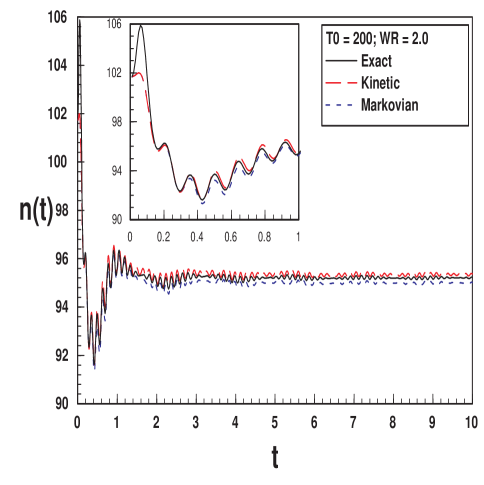
FIG. 2.: The expectation value of the particle occupation number given by eq.(2) for $\Omega=\omega_{p}$ for the case in which the pole is below threshold for particle temperature $T_{0}=200$ and bath temperature $T=100$. The pole is at $\omega_{p}=1.95719$ and $Z=0.95621$. The numerical parameters are $\eta=0.85$, $\omega_{c}=45,\;\omega_{th}=5$ and $\omega_{R}=2$.

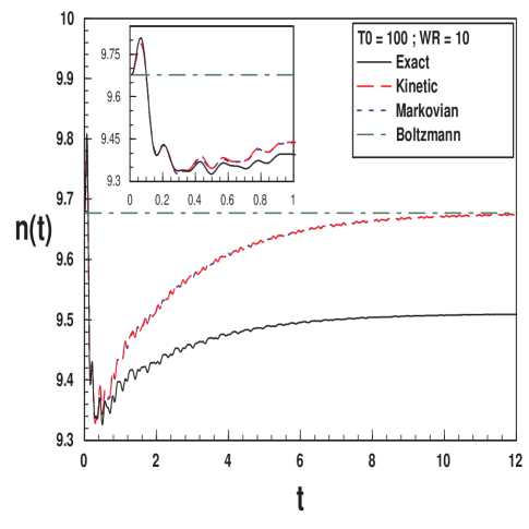
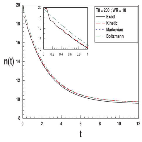
FIG. 3.: The expectation value of the particle occupation number given by eq.(2) for $\Omega=\omega_{p}$ for the case in which the pole is above threshold for particle temperatures $T_{0}=100$ and $200$ and bath temperature $T=100$. The pole is at $\omega_{p}=9.83397$ and $Z=0.99631$. The numerical parameters are $\eta=0.85$, $\omega_{c}=45,\;\omega_{th}=5$ and $\omega_{R}=10$, resulting in $\Gamma/\omega_{p}\approx 0.02$.

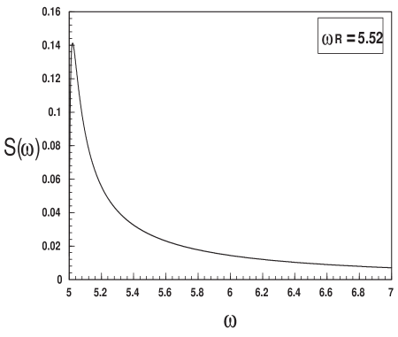
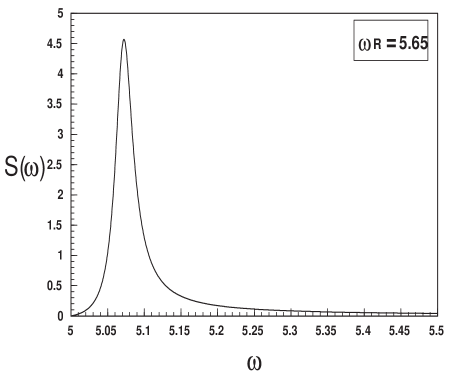
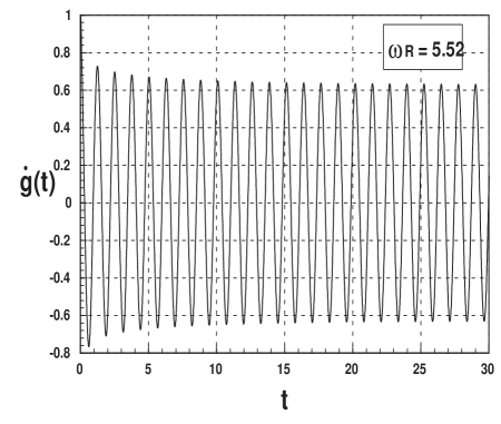
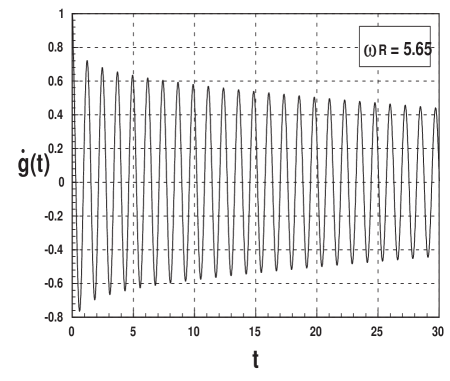
FIG. 4.: The functions $S(\omega)$ and $\dot{g}(t)$ for the cases in which the pole is just below (left column) and just above (right column) the threshold frequency ($\omega_{th}=$ 5). In the left column, $\omega_{R}=5.52,\;\omega_{p}=4.98083$ and $Z=0.63845$ while in the right column $\omega_{R}=5.65,\;\omega_{p}=5.07373$ and $Z=0.69959$. The numerical parameters are $\eta=3.0$ and $\omega_{c}=55$, with $\Gamma/\omega_{p}\approx 0.005$.

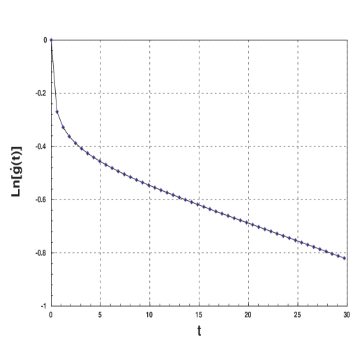
FIG. 5.: The logarithm of the maxima of $\dot{g}(t)$ vs $t$ for $\eta=$ 3.0 and $\omega_{c}=55,\;\omega_{th}=5$, $\omega_{R}=5.52,\;\omega_{p}=4.98083$ and $Z=0.63845$, corresponding to the right column of fig.4.

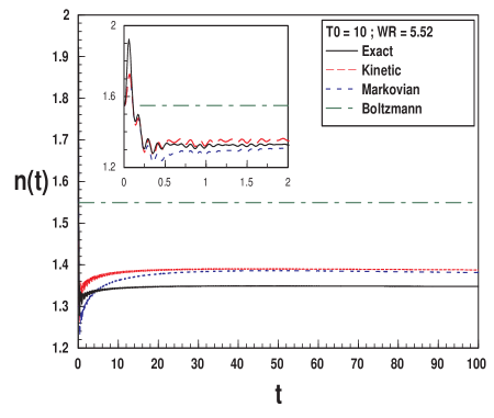
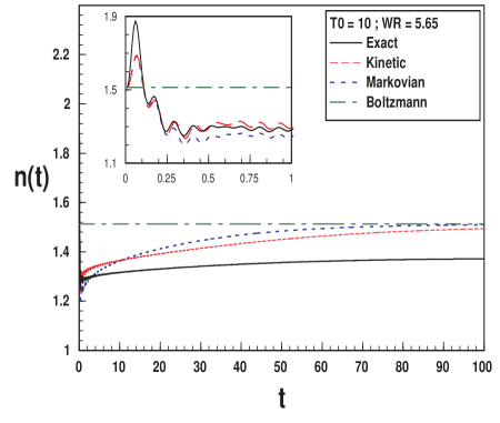
FIG. 6.: The expectation value of the number operator eq.(2) for the same values of the parameters as in figure(4)(left figure corresponds to pole below threshold and right figure to the pole above threshold) for the case of equal particle and bath temperature $T_{0}=T=10$. The insert shows the early time behavior.

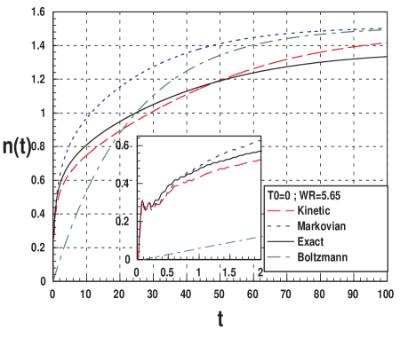
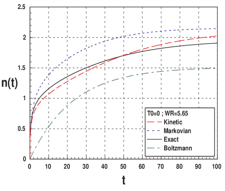
FIG. 7.: The expectation value of the number operator eq.(2) for the same values of the parameters as for the right column in figure(4)(quasiparticle pole above threshold), $\eta=3.0$ and $\omega_{c}=55,\;\omega_{th}=5$, $\omega_{R}=5.65,\;\omega_{p}=5.07373$ and $Z=0.69959$. The temperature of the bath is $T=10$ and zero initial particle temperature ($T_{0}=0$), the exact, Markovian and kinetic curves have been divided by the wave function renormalization $Z$ in the rightmost figure. The insert in the left figure shows the early time behavior.

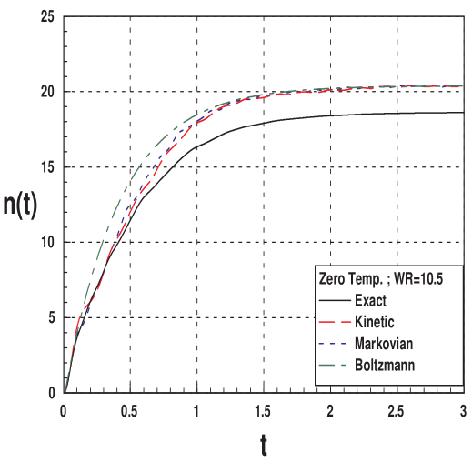
FIG. 8.: The expectation value of the number operator eq.(2) for $\eta=5.0$ and $\omega_{c}=40$, $\omega_{th}=5,\;\omega_{p}=9.58,\;Z=0.982$ and bath temperature $T=200$, corresponding to $\Gamma/\omega_{p}\approx 0.1$.

REFERENCES

- [1] J. Shah, Ultrafast Spectroscopy of Semiconductors and Semiconductor Nanostructures (Springer-Verlag, New York, 1996).
- [2] H. Haug and A. P. Jauho, Quantum Kinetics in Transport and Optics of Semiconductors (Springer, Berlin, 1996).
- [3] S. Bar-Ad et al., phys. Rev. Lett. 77, 3177 (1996); U. Siegner et al., phys. Rev. Lett. 74, 470 (1995); B. Hu et al., phys. Rev. Lett. 74, 1689 (1995).
- [4] F. Camescasse, et al., phys. Rev. Lett. 77, 5429 (1996).
- [5] L. Bányai et al., phys. Rev. Lett. 75, 2188 (1995).
- [6] H. Haug, Phys. Stat. So. (b)173, 139, 1992.
- [7] For a recent discussion of experimental results and theoretical efforts, see the following articles: E. Reittsamer, L. Banyai, D. B. Tran Thoai, P. I. Tamborenea and H. Haug in the proceedings of “ 23rd International Conference on The Physics of Semiconductors” Vol1, page 685 (Eds. M. Scheffler and R. Zimmermann, World Scientific, 1996); D. S. Chemla, ibid, page 625; K. Henneberger, H. Güldner and T. Jäkel, ibid, page 681; M. Wegener et. al. ibid, page 633.
- [8] K. Morawetz and H. S. Köhler, nucl-th/9802082.
- [9] K. Morawetz, V. Špička, and P. Lipavský, physics/9802050 ; K. Morawetz, physics/9802049.
- [10] H. Köhler, Phys. Rev. E 53, 3145 (1996); Phys. Rev. C 51, 3232 (1995).
- [11] P. Danielewicz, Ann. of Phys. (N.Y.) 152, 239, (1984).
- [12] I. D. Lawrie, Phys. Rev. D 30, 3330 (1989). D. Boyanovsky, I. D. Lawrie and D.-S. Lee, Phys. Rev. D 54, 4013 (1996). S.P. Klevansky, A. Ogura, J. Hüfner, Annals Phys. 261, 37 (1997); S.P. Klevansky, A. Ogura, P. Rehberg, J. Hüfner hep-ph/9705321; hep-ph/9701355. P. Rehberg, Phys. Rev. C 57, 3299 (1998).
- [13] C. Greiner and S. Leupold, hep-ph/9802312.
- [14] Daniel Boyanovsky, Hector J. de Vega, Richard Holman, S. Prem Kumar, Robert D. Pisarski, hep-ph/9802370.
- [15] J. Schwinger, J. of Math. Phys. 2, 407 (1961); L. V. Keldysh, Sov. Phys. JETP 20, 1018 (1965).
- [16] L. P. Kadanoff and G. Baym, Quantum Statistical Mechanics (Benjamin, New York, 1962).
- [17] P. Lipavský, V. Špička, and B. Velický, Phys. Rev. B 34, 6933 (1986).
- [18] A. Kuznetsov, Phys. Rev. B 44, 13381 (1991); A. Kuznetsov, Ann. of Phys.(N.Y.) 258, 157 (1997).
- [19] H. Schoeller, Ann. of Phys.(N.Y.) 229, 273 (1994).
- [20] H. Haug, Phys. Stat. Sol.(b) 173, 139 (1992); ibid 149 (1992); D. Tran Thoai and H. Haug, Phys. Rev. B 47, 3574 (1993).
- [21] V. Meden, C. Wöhler, J. Fricke and K. Schönhammer, Phys. Rev. B 52, 5624 (1995). K. Schönhammer and C. Wöhler, cond-mat/9703105 (1997).
- [22] V. Špička and P. Lipavský, Phys. Rev. B 52, 14615 (1995); P. Lipavský, F. Khan, and J. Wilkins, Phys. Rev. B 43, 6665 (1991).
- [23] D. Kremp, M. Bonitz, W. Kraeft, and M. Schlanges, Ann. of Phys.(N.Y.) 258, 320 (1997).
- [24] J. Fricke, Ann. of Phys.(N.Y.) 252, 479 (1996); J. Fricke, V. Meden, C. Wöhler, and K. Schönhammer, Ann. of Phys.(N.Y.) 253, 177 (1997).
- [25] M. Bonitz et. al, J. Phys.: Condens. Matter 8, 6057, (1996)
- [26] P. Ullersma, Physica 32, 27 (1966).
- [27] A. O. Caldeira and A. J. Leggett, Physica A 121, 587 (1983).
- [28] H. Grabert, P. Schramm and G-L Ingold, Phys. Rep. 168, 115 (1988).
- [29] R. Feynman and F. Vernon, Ann. of Phys.(N.Y.) 24, 118 (1963).
- [30] A Schmid, J. Low Temp. Phys. 49, 609 (1982).
- [31] U. Weiss, Quantum Dissipative Systems (World Scientific, Singapore, 1993), and references therein.
- [32] G. V. Efimov and W. von Waldenfels, Ann. Phys. (N.Y.) 233, 182 (1994). I. Joichi, Sh. Matsumoto and M. Yoshimura, Prog. Theo. Phys. 98, 9 (1997); M. Yoshimura, hep-ph/9801423; hep-ph/9702288; cond-mat/9612235;
- [33] K. T. Mahanthappa, Phys. Rev. 126, 329 (1962); P. M. Bakshi and K.T. Mahanthappa, J. Math. Phys. 4, 1,12 (1963); V. Korenman, Ann. Phys. 39, 72 (1966); G. Z. Zhou, Z. B. Su, B. L. Hao, and L. Yu, Phys. Rep. 118, 1 (1985); J. Rammer and H. Smith, Revs. of Mod. Phys. 58, 323 (1986); E. M. Lifshitz and L. P. Pitaevskii, Physical Kinetics (Pergamon, New York, 1981); G. D. Mahan, Many Particle Physics, 2nd ed. (Plenum, New York, 1990); H. Kleinert, Path Integrals in Quantum Mechanics, Statistics and Polymer Physics, 2nd ed. (World Scientific, Singapore, 1996); R. Mills, Propagators for Many Particle Systems (Gordon and Breach, New York, 1969).
- [34] D. Boyanovsky, M. D’Attanasio, H. J. de Vega, R. Holman, Phys. Rev. D 54 1748 (1996); D. Boyanovsky, M. D’Attanasio, H. J. de Vega, R. Holman, D.-S. Lee, Phys. Rev. D 52 6805 (1995).
- [35] P. Noziéres, Interacting Fermi Systems (Benjamin, Reading, Mass., 1964).
- [36] P. Lipavský, F. S. Khan and J. W. Wilkins, Phys. Rev. B43, 6665 (1991).