[

Stripes and the t-J model

Abstract

We investigate the two-dimensional t-J model at a hole doping of $x=\frac{1}{8}$ and $J/t=0.35$ with exact diagonalization. The low-energy states are uniform (not striped). We find numerous excited states with charge density wave structures, which may be interpreted as striped phases. Some of these are consistent with neutron scattering data on the cuprates and nickelates.

]

In the search for an understanding of the cuprate superconductors it is desirable to find a model which captures many of the essential aspects of the environment experienced by the electrons in these materials. Because these materials are born out of antiferromagnetic insulators by doping, it is somewhat urgent to decide if a simple model which begins from the strong electron correlation limit, such as the so-called t-J model, can explain some features which result from the electronic degrees of freedom in the cuprates[3]. Even though the progress made in trying to solve the t-J model may be characterized as slow, it gives some features which are present in these materials. For example, some important aspects of the calculated single-hole spectrum[4] are in agreement with the results of the photo-emission data[5]. In addition, the model gives rise to a two-hole bound state[6] with the $d_{x^{2}-y^{2}}$ symmetry which is the believed symmetry of the superconducting state in these materials.

Emery and Kivelson[7] suggested that the cuprates are near an electronic phase separation instability which is prevented by the long-range part of the Coulomb interaction. In the phase-separated state, the holes cluster together, leaving the rest of the system in an antiferromagnet state with no holes. Phase separation in the t-J model has been studied by a number of techniques which seem to be giving conflicting conclusions[8, 9, 10, 11, 12]. For example, Hellberg and Manousakis[8] using a stochastic projection method, an extension of the Green’s function Monte Carlo (GFMC) for lattice fermions, find that the t-J model has a region of phase separation at all interaction strengths. Other techniques fail to reach this conclusion. Most of these studies use small size systems[9], high temperature series expansions[10], or approximate methods[11, 12]. In a very recent calculation Calandra et al.[12] using the GFMC approach within the fixed node approximation find that the phase boundary for phase separation is far from that determined by the high temperature series expansions [10] and much closer to that obtained by Hellberg and Manousakis [8] except in the delicate region with small hole dopings and $J/t\lesssim 0.4$. By using a uniform Fermi-liquid type nodal structure one disregards the possibility of a non-uniform ground state in which one component of the mixture (the antiferromagnetic phase) has no fermion degrees of freedom. In addition, in the delicate region of small $J/t$ and low doping, Shraiman and Siggia[13] and Boninsegni and Manousakis[14] showed spin-back-flow effects become very important resulting in the interesting structure of the hole “polaron”. These effects are known to change the nodal structure of the wave function in a crucial way in strongly correlated quantum fluids. Therefore fixed-node GFMC may be inadequate in this region.

The phase separation in the t-J model cannot be realized in the physical system due to the Coulomb interaction[7, 8, 15]. Instead such a tendency for phase separation can be satisfied locally by forming stripes or other charge density wave (CDW) structures without a large Coulomb cost. The coupling of electrons to lattice distortions may also encourage the formation of stripes.

Experimentally, stripe modulations were first observed in a doped nickelate analogue of the cuprates [16]. La₂NiO₄ may be doped with holes by adding oxygen or by substituting strontium for lanthanum. The modulation seen with neutron scattering in the doped compounds is consistent with the holes forming diagonal domain walls separating antiferromagnetic regions of spins. Stripes with a variety of widths and hole densities along the stripes have been observed.

There is strong evidence for stripe modulations in the cuprates as well[17]. In La_1.6-xNd_0.4Sr_xCuO₄, superconductivity is suppressed at a filling of $x=\frac{1}{8}$, and neutron scattering studies reveal vertical domain walls of holes and spins. In these stripes, a hole density of $\rho_{h}=1/2$ per lattice spacing is observed.

Recently White and Scalapino (WS) found static vertical stripe order similar to that of the cuprates in the two-dimensional t-J model using a density matrix renormalization group technique [18]. These results are surprising due to the fact that the t-J model ignores the long-range part of the Coulomb interaction and couples to no lattice distortions. One sees no physical reason for such a simplified model to have a ground state with a periodic array of interfaces.

In this paper we study the two-dimensional t-J model at a hole doping of $x=\frac{1}{8}$ and at $J/t=0.35$ with exact diagonalization. The low-energy states are uniform (not striped). We find a variety of CDW excited states which may be interpreted as striped phases. Some of these are in excellent agreement with neutron scattering data on the cuprates and the nickelates. However, without adding additional terms to the t-J model, such as a long-range Coulomb interaction or a coupling to the lattice, the striped states are only realized as excited states.

The t-J Hamiltonian is written in the subspace with no doubly occupied sites as

$$H=-t\sum_{\langle ij\rangle\sigma}(c_{i\sigma}^{\dagger}c_{j\sigma}+{\rm h.c.})+J\sum_{\langle ij\rangle}({\bf S}_{i}\!\cdot\!{\bf S}_{j}-\frac{n_{i}n_{j}}{4}).$$ (1)

Here $\langle ij\rangle$ enumerates neighboring sites on a square lattice, $c_{i\sigma}^{\dagger}$ creates an electron of spin $\sigma$ on site $i$, $n_{i}=\sum_{\sigma}c_{i\sigma}^{\dagger}c_{i\sigma}$, and ${\bf S}_{i}$ is the spin-$\frac{1}{2}$ operator. Throughout this paper, we take $t=1$ and $J=0.35$.

To achieve a doping of $x=\frac{1}{8}$, all calculations were carried out on periodic 16-site clusters with two holes. Periodic clusters may be characterized by their primitive translation vectors a₁ and a₂. There are a large number of possible 16-site clusters on the two-dimensional square lattice. Each cluster can only support striped phases that are commensurate with the periodicity of that particular cluster[19]. Clusters which have one particularly short translation vector are quasi-one-dimensional and behave like chains or ladders. We only consider clusters in which both translation vectors have a Manhattan length of at least $l_{M}=|a^{x}|+|a^{y}|\geq 4$. There are seven such clusters, shown in Table I. These clusters represent all possible quasi-two-dimensional 16-site clusters. Later in the paper, we examine six eigenstates in detail. We label these states by letters, (a) through (f), shown next to their corresponding clusters in Table I.

TABLE I.: Translation vectors of the seven possible quasi-two-dimensional 16-site clusters. The letters label eigenstates examined later in the paper.

Number	a1	a2	States
1	(0,4)	(4,0)
2	(0,4)	(4,1)	(e),(f)
3	(0,4)	(4,2)
4	(3,2)	(2,-4)
5	(3,1)	(1,-5)	(d)
6	(2,2)	(4,-4)	(a),(b)
7	(2,2)	(3,-5)	(c)

We studied all eigenstates with energy per site ${\cal E}<-0.634$ for each of the seven periodic clusters. For each cluster, we use all possible combinations of phases $\theta=0,\pi$ along each translation vector. Several of these states are CDWs, which are necessarily degenerate. The density in a CDW state is characterized by an amplitude $A$, a wave-vector k, and an arbitrary phase $\phi$. The phase $\phi$ depends on the particular linear combination of degenerate states taken. Thus the hole density on site ${\bf r}_{i}$ is given by

$$n_{h}({\bf r}_{i})=\bar{n}_{h}+A\cos({\bf k}\cdot{\bf r}_{i}+\phi),$$ (2)

where the average hole density is $\bar{n}_{h}=\frac{1}{8}$.

FIG. 1.: Amplitude of the CDW in every state with energy per site ${\cal E}<-0.634$. The six labeled states correspond to states examined in detail later in the paper. The low-energy states have no CDWs.

The amplitude $A$ of the CDW in every low-energy state are plotted in Fig. 1 as a function of energy per site. The lowest energy states are uniform and have CDW amplitude $A=0$. For energies above ${\cal E}\gtrsim-0.645$ some CDW states are stabilized. The maximum CDW amplitude of these states increases with increasing energy.

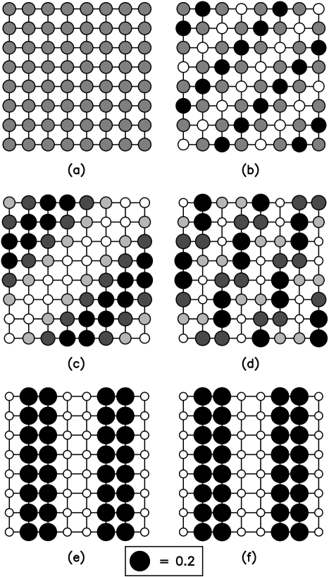
FIG. 2.: Hole structures of the six eigenstates we chose to examine in detail. The radius of each circle is proportional to the hole density on the given site. Additionally, the circles are shaded according to the relative hole density in each state: Black circles show the maximal hole density in that state while white circles show the minimum. State (a), which has the minimum energy, has a uniform hole density. States (b) through (f) have increasing energy and show increasing CDW amplitude. In all states the average spin moment on each site is zero.

We examine in detail the six labeled states in Fig. 1. State (a) is the lowest energy state and is uniform. States (b) through (f) have increasing CDW amplitude and increasing energy. Each of these states has the largest CDW amplitude of all states at or below its energy.

We examine the charge order of the six states in Fig. 2. The CDW states, (b) through (f), are degenerate, so taking a different linear combination of the eigenstates will move the CDW. In particular, in state (b) the maximum charge order occurs on a site, while in states (c), (d), (e), and (f), the maximum charge order occurs between two sites, or on a bond. All of the states have site-centered and bond-centered CDWs with different linear combinations.

States (b) and (c) have diagonal stripes with two different hole densities along the stripe. State (b) has hole density $\rho_{b}=1/2$ per (1,1) step, while state (c) has $\rho_{c}=1$. These states are similar to experimental results on the nickelates [16] and to the mean-field calculations of Zaanen and Littlewood[20].

States (e) and (f) exhibit vertical stripes with 1/2 hole per (0,1) step consistent with experimental results on La_1.6-xNd_0.4Sr_xCuO₄ [17] and with the calculations of WS[18]. States (e) and (f) have the largest CDW amplitudes that we found.

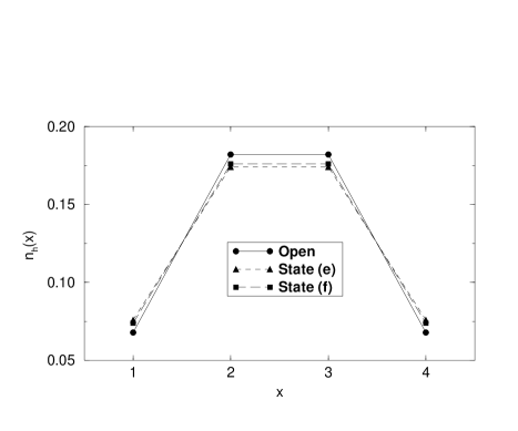
FIG. 3.: Comparison of the hole density $n_{h}$ as a function of $x$-coordinate for a $4\times 4$ cluster with open boundary conditions in the $x$-direction and states (e) and (f). All three systems have exhibit a stripe in the $y$-direction. The state with open boundary conditions is the non-degenerate ground state.

Interestingly, the CDWs of the vertical stripe states, (e) and (f), are remarkably similar to the density profile obtained from the ground state of a $4\times 4$ cluster with open boundary conditions in the $x$-direction and periodic boundary conditions in the the $y$-direction, the boundary conditions used by WS[18]. The hole density as a function of the $x$-coordinate for these three states is shown in Fig. 3. The states (e) and (f) are excited states of the periodic cluster #2 in Table I. The $4\times 4$ cluster with open boundary conditions in the $x$-direction can be generated from the periodic cluster #2 by cutting all bonds along one column. Clearly, the excited states (e) and (f) essentially have an extra node along one column. The open boundary conditions in one direction causes the ground state of this cluster to be very similar to excited states of the periodic cluster. The open boundary conditions select the striped state to be the ground state.

None of the eigenstates has a spontaneous spin density wave amplitude, but the spin correlations are affected by the CDW. One way to show the spin correlations is to apply small magnetic fields along the boundary of the simulation cell, as done by WS[18]. This is shown for the diagonal and vertical stripe states (b) and (f) in Fig. 4. The stripes are pinned so the sites with the fields have maximum electron density with the appropriate average polarization. In both the diagonal and vertical cases, the antiferromagnetic order in neighboring stripes is shifted by $\pi$, as in the nickelates and cuprates[16, 17].

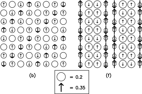
FIG. 4.: Hole and spin structures of states (b) and (f) generated by applying a small staggered magnetic field of $h=0.1$ to sites at the boundary of the simulation cell to pin the spins. The radius of each circle is proportional to the hole density on the given site, and the length of the arrows is proportional to $\langle S^{z}_{i}\rangle$. These are not eigenstates of the t-J Hamiltonian without the pinning fields, but the spin correlations pictured are similar to the correlations in the eigenstates (b) and (f). State (e) has a spin and charge structure very similar to state (f) and is not shown.

To conclude, we found stripes in the t-J model at a doping of $x=\frac{1}{8}$, but only as excited states. The ground state of the model for $J/t=0.35$ is uniform. The energy cost per site to form diagonal stripes similar to those found in the nickelates is at least $\Delta_{d}\gtrsim 0.016t$, and for vertical stripes similar to those in the cuprates the energy cost is $\Delta_{v}\gtrsim 0.025t$. At this doping and interaction strength studies on larger systems have found that the model is nearly phase separated[8]. The stripes seen experimentally could be the result of phase separation frustrated by the Coulomb repulsion[15] and/or the coupling of the electrons to lattice distortions. However, the stripe states are not ground states of the simple t-J model, as claimed in Ref. [18].

Our findings are in agreement with the recent work of Pryadko, Kivelson and Hone[21] who studied the interaction between localized holes in a weakly doped quantum antiferromagnet. They find that stripes are unstable due to an attractive interaction between such domain walls.

We thank R.E. Rudd and Steve Kivelson for numerous stimulating conversations. This work was supported by the Office of Naval Research Grant No. N00014-93-1-0189, and by the National Research Council. The calculations were performed on the SP2 at the DoD HPC Aeronautical Systems Center Major Shared Resource Center at Wright Patterson Air Force Base.

REFERENCES

- [1] Electronic address: hellberg@dave.nrl.navy.mil
-
[2]
Electronic address: stratos@samos.martech.fsu.edu
Web address: www.stratos.fsu.edu - [3] E. Manousakis, Rev. Mod. Phys. 63, 1 (1991).
- [4] Z. Liu and E. Manousakis, Phys. Rev. B 45, 2425 (1992).
- [5] B.O. Wells et al., Phys. Rev. Lett. 74, 964 (1995).
- [6] M. Boninsegni and E. Manousakis, Phys. Rev. B 47, 11897 (1993).
- [7] V.J. Emery, S.A. Kivelson, and H.Q. Lin, Phys. Rev. Lett. 64, 475 (1990); S.A. Kivelson, V.J. Emery, and H.Q. Lin, Phys. Rev. B 42, 6523 (1990); S.A. Kivelson and V.J. Emery, in Strongly correlated electronic materials: the Los Alamos symposium, 1993, edited by K.S. Bedell et al. (Addison-Wesley, Reading, CA, 1994).
- [8] C.S. Hellberg and E. Manousakis, Phys. Rev. Lett. 78, 4609 (1997).
- [9] E. Dagotto, Rev. Mod. Phys. 66, 763 (1994); H. Fehske, V. Waas, H. Röder, and H. Büttner, Phys. Rev. B 44, 8473 (1991); D. Poilblanc, ibid. 52, 9201 (1995).
- [10] M.U. Luchini, et al., Physica C 185-189, 141 (1991); W.O. Putikka, M.U. Luchini, and T.M. Rice, Phys. Rev. Lett. 68, 538 (1992).
- [11] M. Kohno, Phys. Rev. B 55, 1435 (1997);
- [12] M. Calandra, F. Becca and S. Sorella, e-print, Cond-mat/9810301.
- [13] B. Shraiman and E. Siggia, Phys. Rev. Lett. 60, 740 (1988) and ibid. 61, 467 (1988)
- [14] M. Boninsegni and E. Manousakis, Phys. Rev. B 45, 4877 (1992) and ibid., 46, 560 (1992).
- [15] V.J. Emery and S. A. Kivelson, Physica C 209, 597 (1993).
- [16] P. Wochner, J.M. Tranquada, D.J. Buttrey, and V. Sachan, Phys. Rev. B 57, 1066 (1998); S.-H. Lee and S-W. Cheong, Phys. Rev. Lett. 79, 2514 (1997); J.M. Tranquada, D.J. Buttrey, V. Sachan, and J.E. Lorenzo, ibid 73, 1003 (1994); V. Sachan, D.J. Buttrey, J.M. Tranquada, J.E. Lorenzo, and G. Shirane, Phys. Rev. B 51, 12742 (1995); J.M. Tranquada, J.E. Lorenzo, D.J. Buttrey, and V. Sachan, ibid 52, 3581 (1995).
- [17] M.v. Zimmermann, et. al., Europhys. Lett., 41 629 (1998); J.M. Tranquada, et. al., Phys. Rev. Lett. 78, 338 (1997); J.M. Tranquada, et. al., Phys. Rev. B 54, 7489 (1996); J.M. Tranquada, et. al., Nature 375, 561 (1995).
- [18] S.R. White and D.J. Scalapino, Phys. Rev. Lett. 80, 1272 (1998).
- [19] P. Prelovšek and X. Zotos, Phys. Rev. B 47, 5984 (1993).
- [20] J. Zaanen and P.B. Littlewood, Phys. Rev. B 50, 7222 (1994).
- [21] L. P. Pryadko, S. Kivelson and D. W. Hone, Phys. Rev. Lett, 80, 5651 (1998).