Random Magnetic Interactions and Spin Glass Order Competing with Superconductivity: Interference of the Quantum Parisi Phase

Abstract

We analyse the competition between spin glass (SG) order and local pairing superconductivity (SC) in the fermionic Ising spin glass with frustrated fermionic spin interaction and nonrandom attractive interaction. The phase diagram is presented for all temperatures $T$ and chemical potentials $\mu$. SC–SG transitions are derived for the relevant ratios between attractive and frustrated–magnetic interaction. Characteristic features of pairbreaking caused by random magnetic interaction and/or by spin glass proximity are found. The existence of low–energy excitations, arising from replica permutation symmetry breaking (RPSB) in the Quantum Parisi Phase, is shown to be relevant for the SC–SG phase boundary. Complete 1-step RPSB-calculations for the SG–phase are presented together with a few results for $\infty$–step breaking. Suppression of reentrant SG - SC - SG transitions due to RPSB is found and discussed in context of ferromagnet - SG boundaries. The relative positioning of the SC and SG phases presents a theoretical landmark for comparison with experiments in heavy fermion systems and high $T_{c}$ superconductors. We find a crossover line traversing the SG–phase with $(\mu=0,T=0)$ as its quantum critical (end)point in complete RPSB, and scaling is proposed for its vicinity. We argue that this line indicates a random field instability and suggest Dotsenko–Mézard vector replica symmetry breaking to occur at low temperatures beyond.

I Introduction

The goal of this paper is to present a phase diagram describing the competition between spin glass order and superconductivity for cases, which are perhaps best introduced by the example of Heavy Fermion Systems (HFS)[1, 2, 3]. Experiments provided evidence for the fact that the same type of fermions appeared to be responsible for both superconductivity and spin glass order [2]. If one extends this problem of competition and coexistence between magnetism and superconductivity to include as well antiferromagnetism for cases of almost absent disorder or of too small frustration, even more examples for the necessity of single fermion species models can be found, including high-$T_{c}$ superconductors [4, 5, 6].
We wish to address the competition and coexistence problem of SG versus SC-ordering in the context of a many fermion model which appears to be particularly adapted to this kind of problems.
Interacting many fermion systems are famous for their complicated interplay of low–lying excitations of various kinds. Soft breaking of continuous symmetries and Ward identities are at their origin. For the Sherrington-Kirkpatrick Ising spin glass with spin variables living on Fock space, a similar scenario - even if restricted to low–lying single fermion excitations - may come as a surprise, since the Ising model has only $Z_{2}$ symmetry and hence misses the continuous symmetry in spin space, which guarantees soft spin modes in case of Heisenberg models. It is thus important to realize that it needs the full Parisi replica permutation symmetry breaking (RPSB) as a minimum requirement to recover the true quantum–dynamics of fermion correlations in the infinite range fermionic Ising spin glass. Without any further model–ingredient like fermion hopping or Glauber dynamics for example, the fermionic Ising spin glass joins static spin behaviour on one side with a complete quantum–dynamic scenario in its fermion Green’s functions on the other, just as in standard interacting many–fermion systems. Once the fermionic spin glass becomes a part of more general model Hamiltonians, these features infiltrate all coupled degrees of freedom. In this paper, we derive consequences of this very fact for the case of a competing superconducting instability.
On the basis of the proof of soft modes [7], calculations of one-step Parisi RPSB, which already cover more than half of the total correction obtained from infinitely many steps, are often sufficient to guess the correct result, i.e. to imagine important features of the exact solution. Recalling the crucial importance of the presence or absence of soft modes, it is clear that once the Ising spin glass with gaussian distributed exchange interaction is involved in more complicated many fermion models, it plays a role very different from the pure Ising model. We remark that a standard Ising spin glass coupled to a fermionic system by a Kondo interaction constitutes a different case.
The competition between spin glass order and superconductivity has often been considered to arise as a coupling effect between two systems, one of which undergoes magnetic order while the other one eventually becomes superconducting. This issue was addressed by a number of groups in the recent years [8, 9, 10]. If one considers metallic conduction instead of superconductivity one can also find results, obtained along the same lines and with similar modeling, for example described in the book by Fischer and Hertz [11].
In addition to provide a theory close to the conditions of HFS, we intend to present our theoretical statements such that a comparison with phase diagrams of HighTcSuperconductors (HTS) showing a spin glass phase in between the antiferromagnetic and superconducting ones [1, 4, 6, 12] becomes possible. Of course this requires to discuss a classification of more or less robust properties against (low–)dimensional fluctuations.
Strontium doped HTS are the most prominent examples, where antiferromagnetism gives way to clear signatures of spin glass (SG) like behaviour before superconductivity sets in at higher (hole)-doping. A typical SG order parameter was identified at moderately low temperatures [4] $T<8K$ and even an infiltration within the superconducting domain at lowest temperatures was described [6]. Classes of HTS exist as well, which do neither seem to show spin glass nor intermediate phases. It is within the scope of our theory to derive conditions and features, which are specific and in some cases universal. This should provide a means to identify similar behaviour in real systems.
Existence and nature of intermediate spin glass or SG-alike phases in a certain doping range must be expected for example to be important features of strongly correlated systems. Experiments revealing close relations between magnetism and superconductivity in heavy fermion systems addressed coexistence, phase separation, and pairbreaking of local pairs by frozen moments for example [1, 2].
Most of recent theories for HTS materials focussed on the destruction of antiferromagnetism under doping. Viewing an intermediate phase from the superconducting side, the appealing concept of a nodal liquid [13] was developed. The role of quenched disorder and randomness was not yet considered, but its presence should very well participate in the fluctuation destruction of superconductivity. Since we wish to deal in this paper with superconducting transitions under participation of a spin glass, a disorder model is a natural choice. Arguments on an important role of disorder in HTS and in HF-systems were provided experimentally and by theoretical reasoning [1, 5, 2]. Aspects such as non Fermi liquid behaviour, seen to arise in the vicinity of spin glass order [9], also support this point of view.
In this article we present detailed results for spin glass to superconductor transitions in a single-species fermionic model, which treats frustrated magnetic and attractive interaction on the same footing. Unique features of the phase diagram are derived analytically and numerically. The domain of applicability of our model to two-species models, as recently proposed [10] by integrating out conduction electrons coupled to the fermionic spin glass, depends on the Kondo–effect and whether the magnetic moments forming the glassy order become quenched or not. This needs further analysis. We discuss below a related case emerging in the Periodic Anderson Model in section XI. In terms of our presentation as a single–species model the problem of quenched moments appears in form of a metallic spin glass - paramagnet transition.
For the present one–species model we shall observe that for certain interaction ratios the location of the spin glass bears resemblance to that of a logarithmic resistivity regime residing above a spin glass ordered phase at lower $T$ in Sr-doped HTS [4, 5]. A fluctuational state of broken down spin glass order - perhaps due to low dimensionality - should contribute to transport properties seen in intermediate phases above $T_{f}$. In particular, SG order was recently shown to affect transport properties strongly[14], an effect that can well have a weak localization precursor due to the random magnetic interaction.
A HTS mechanism related to magnetic fluctuations of a broken down spin glass appears possible and studies thereof quite justified.

II Outline of the paper

The paper covers the different issues of one–step replica symmetry breaking in the Sherrington–Kirkpatrick model on Fock space, the extension of the local theory of disordered superconductivity to arbitrary filling, and finally the competition between glassy magnetic order and superconductivity.
It is organized in three interrelated larger pieces.
I. Several 1–step RPSB solutions for the fermionic Ising spin glass are presented in section VI. The discovery of a new random field instability traversing the entire spin glass phase is exposed by the crossover line Figure 4 of section VI.
The new 1–step RPSB solutions serve to evaluate the free energies in the $(\mu,T)$–plane required to obtain the superconductor spin glass phase diagram in the final part of the paper.
II. In two intermediate sections, VII and VIII, we report progress obtained by means of the computer algebra program Mathematica for the local theory of superconductivity.
This local theory adapts to some of the basic conditions of disordered heavy fermion systems.
This part also emphasizes the relation with the $d=\infty$-technique for clean systems. In these sections, we take explicitly into account fermion hopping effects, which become dominant in the low temperature part of the superconducting phase. In the rest of the paper we focus on superconductivity arising in the magnetic band generated by the frustrated magnetic interaction, which is also responsible for spin glass order emerging under favourable conditions.
III. Sections IX and X contain the SG - SC phase diagram. We chose to consider the competition problem between SG and SC order under the condition of a hopping band small in comparison with the magnetic band generated by the frustrated magnetic interaction, which renders corrections from fermion hopping negligible. Preliminary discussions are given in section V and the final result is that of Figure 13. We compare this phase diagram with the wellknown ferromagnet - spin glass diagram (see for example Ref.[15]). In order to see the relationship, one only needs to replace first the ferromagnetic- by the attractive interaction and, secondly, the magnetic field by the chemical potential (note: by means of a partial particle–hole transformation, one may convert the chemical potential back into a magnetic field, but then the frustrated magnetic interaction would turn into a charge interaction reflecting thus the basic difference). The shape of the SG - SC phase diagram shown in sections IX and X confirms the genuine features.

III Main results

1. One of the main results and the motivation of this paper is the derivation of the phase diagram for a fermion system with competing frustrated magnetic interaction and superconducting order in sections IX and X. Our final answers can be found in the Figures 6, 7 (replica–symmetric approximation) and finally in Figures 11-13 including symmetry breaking effects. The phase diagram can be viewed in connection with the famous classical counterpart of spin glass - (anti)ferromagnet boundaries [15]. Several different features arise, but a common one to both cases is the suppression of reentrant behaviour due to replica permutation symmetry breaking, evidenced by Figure 13.
2. As intermediate steps we derived novel one–step RPSB results for the order parameters for all temperatures and for a wide range of chemical potentials by extremalizing the free energy in a fourdimensional parameter space, as reported here. In a five–dimensional space we determined a crossover line indicating
3. a new type of random field instability.
This part is also new for the pure spin glass problem irrespective of the competition with superconductivity. The features of this instability deserve separate attention in another publication. We report only those parts needed to resolve the superconductivity coexistence problem and some features related to the appearence of a new Quantum Critical Point (QCP).
4. Also as intermediate steps to achieve the main goal, we derive a couple of new results for the theory of superconductivity with local Wegner invariance[16] in sections VII and VIII. This type of superconductivity is marked by a two–particle phase coherence length playing a very similar role as the usual one–particle coherence length (the latter one being suppressed by local invariance which results under the disorder ensemble average).
5. We obtain several exact results and relations for both the superconductivity and the spin glass issues. We consider as a nice example the results for the normal and anomalous Green’s functions, expressed in terms of the Kummer function (also known as Hypergeometric U-function), which display a unique type of spin glass pairbreaking effect (due to the proximity in the phase diagram). One may view this also as the effect of the random magnetic interaction within the superconducting phase.
6. With these results we evaluate the complete crossover from BCS to Bose condensation type superconductivity (see Figure 10), the crossover being controlled by the ratio of hopping bandwidth and attractive interaction. Similarities between the effects which the local Wegner invariance has on disordered superconductivity and those of the $d=\infty$–technique, usually applied to the Hubbard model, are remarked.

IV The model

We consider here a model described by the grand canonical Hamiltonian

$${\cal{K}}\equiv{\cal{H}}_{Jv}+{\cal{H}}_{t}-\mu\sum n_{i},$$ (1)

composed of

$${\cal{H}}_{Jv}=-\frac{1}{2}\sum J_{ij}\sigma_{i}\sigma_{j}-\sum v_{ij}a_{i\downarrow}^{\dagger}a_{i\uparrow}^{\dagger}a_{j\uparrow}a_{j\downarrow},$$ (2)

$$\hskip 56.9055pt{\cal{H}}_{t}=\sum_{ij\sigma}t_{ij}a_{i\sigma}^{\dagger}a_{j\sigma},$$ (3)

where $\sigma_{i}=n_{i\uparrow}-n_{i\downarrow}$, $a_{i\sigma}$, $n=n_{\uparrow}+n_{\downarrow}$ denote spin, fermion, and fermion-number operators respectively. The variance $J^{2}$ of the frustrated, infinite-ranged and Gaussian–distributed magnetic interaction $J_{ij}$ and its magnitude relative to that of the attractive coupling, $v_{q=0}/J$ are relevant parameters below, together with the chemical potential and the related filling factor $\nu(\mu)$. We do not restrict the attractive interaction to be local, which would mean a negative $U$ Hubbard interaction. Quantum spin-dynamics would then exclusively be linked to the fermion hopping $t_{ij}$. The mean field approximation may of course be viewed as exact in the limiting cases of either infinite-ranged $v_{ij}$, infinite number of orbitals per site, or in the case of infinite dimensions. In the latter limit the one particle Green’s functions become site-local in the similar way as in the ensemble average for the present model. The nonlocal and translationally invariant attractive interaction $v_{i-j}$, which allows for pair-hopping, is compatible with the site-local property. We note that local pairing on the average does not prevent BCS-like behaviour as can be seen for example explicitly from the discussion below. The model fits particularly cases encountered in HFS, where one fermion species appears to be responsible for superconductivity and magnetism.
We restrict the discussion to the small $t/J$ regime, which implies that the selfconsistently determined magnetic band is much larger than the hopping bandwidth in general. Only deep within the superconducting regime, where the magnetic bandwidth almost shrank to zero, the single fermion hopping bandwidth becomes dominant.
Local pairs can be delocalized due to finite range $v_{ij}$ or by arbitrarily weak fermion hopping $t_{ij}$. We employ a local pairing theory of superconductivity based on the order parameter $\Delta\equiv\langle a_{i\uparrow}a_{i\downarrow}\rangle$, and on a two-particle coherence length replacing the usual one-particle length in the corresponding Ginzburg-Landau theory.

V The basic selfconsistency equations of the fermionic Ising spin glass with superconducting order

We begin this paper with the insulating fermionic Ising spin glass with an additional local pairing order parameter $\Delta$. The theoretical foundation of the fermionic Sherrington Kirkpatrick Ising spin glass in the plane of complex chemical potential is quite rich. Many features had been elucidated in previous papers and thus only the important facts needed to understand the present work should be repeated. In contrast to the standard classical Sherrington Kirkpatrick model, which is realized for example at $\mu=i\pi T/2$ in the set of grand–canonical fermionic Ising spin glasses defined with complex chemical potential, the continuous subset on the real $\mu$ axis has two faces: a static one for all spin and charge–correlations and a quantum–dynamic one for the fermion correlators like Green’s function etcetera. This led us recently to discover the Quantum–Dynamical Parisi Phase in this parent model to many other ones in theory of disordered interacting fermion systems.
A rather wellknown and frequently considered source of quantum spin–dynamics has been the transverse field in models defined on spin space [17, 18, 19]. It should be evident for the reader that the fermionic Ising spin glass, complemented with a decoupled attractive fermion interaction to allow for superconducting order, also develops quantum spin dynamics. This holds true after mean–field decoupling of the attractive interaction with a finite superconducting order parameter $\Delta$, since the anomalous term does not commute with the Ising Hamiltonian. There will also emerge quantum dynamical behaviour in charge correlations and most important, the underlying quantum–dynamical Parisi features of the single– and many–fermion propagators are involved too. Thus the fermionic Ising spin glass with just superconducting order contains already more physics than any quantum spin glass in the traditional sense, since the latter models are all represented on the imaginary $\mu$–axis and their fermions are not real physical objects.
Quantum–dynamical effects are usually dealt with in an approximate way, a very good analytical idea - depending on the application one has in mind - being the one of Fedorov and Shender [20], another one developed by Subir Sachdev for Ginzburg Landau theories [19] and employed for the metallic spin glass too [21]. Unlike the Heisenberg model, where Usadel proved the importance of spin dynamics for the absence of replica-symmetric domains within the spin glass phase [22], spin–dynamical corrections to the Ising spin glass - superconductor boundary are negligible. On the contrary replica symmetry breaking is linked to the quantum fermion dynamics and turns out to be essential at low temperatures. Our results presented in section X show that it suppresses reentrant SG - SC - SG transitions. The latter point of course recalls what has been found for the ferromagnetic - spin glass boundary in the Sherrington–Kirkpatrick model [15].
The effects of Parisi’s RPSB complicate the appearance and the treatment of the selfconsistency equations such that it is necessary to start with the unbroken simpler ones. Already these equations turn out to have multiple solutions, whose stability changes eventually as a function of chemical potential and temperature. The stable solutions must first be understood before the one step RPSB analysis can be started.

A The free energy and resulting selfconsistency equations in replica symmetric approximation

The grand canonical model ${\cal{H}}_{Jv}$ can be decoupled in the standard way. The Grassmann field theory depends on how many steps of replica symmetry breaking are taken care of - hardly necessary to say that one can rarely hope to find full analytical solutions. Already one–step breaking is nonsimple and in case of the fermionic model is almost as complicated as two–step breaking in the standard case on spin space. Let us start with the free energy obtained in the replica symmetric and $Q$–static approximation as

$$f=\frac{1}{4}\beta J^{2}((\tilde{q}-1)^{2}-(q-1)^{2})+\frac{|\Delta|^{2}}{v}-T\ln 2-\mu-T\int_{z}^{G}\ln{\cal{C}},$$ (4)

where

$${\cal{C}}(z)\equiv\cosh(\beta\tilde{H}(z))+\cosh(\beta\sqrt{\mu^{2}+|\Delta|^{2}})\exp(-\frac{1}{2}(\beta J)^{2}(\tilde{q}-q))\quad\mbox{and}\quad\tilde{H}(z)\equiv J\sqrt{q}z$$ (5)

Here, we have introduced the convenient short–hand notation for the Gaussian integral operator

$$\int_{z}^{G}=\frac{1}{\sqrt{2\pi}}\int_{-\infty}^{\infty}dz\exp(-z^{2}/2).$$ (6)

The dynamic susceptibility $\chi(\omega)$ is approximated by the $\omega=0$–part denoted by $\tilde{q}\equiv\chi(\omega=0)\hskip 2.84544ptT$, an approximation which becomes exact however for vanishing superconducting order parameter. Thus the equations are sufficient to determine the replica symmetric phase boundary. Even in case of discontinuous transitions, dynamic corrections are very small, first as long as the jump of superconducting order parameter rests small, second because the free energy integrates over the dynamic effects of Lorentzian broadening [20]. No qualitatitive change can thus be expected from this type of dynamics. Deeper inside the superconducting phase the calculation with the static $<\sigma_{i}(t)\sigma_{i}(t^{\prime})>$ becomes approximative but still interesting. The exact mean field solutions are much more involved than those known from the pairbreaking effects of random magnetic impurities, the latter case being included in section VIII. We hope to come back to the dynamic corrections around the new solutions so far obtained in $\chi(\omega)\approx\chi(0)=\beta\tilde{q}$ approximation.
As the superconducting order increases the susceptibility $\chi$ is depressed strongly and using the static approximation for $\chi(\omega)$ again does not deteriorate the treatment. All this will be worked out below in the section VII of local pairing superconductivity with the local Wegner - invariance.
Comparing with the transverse field Ising model, it is here the superconducting order parameter - or, if one looks at the original model, the attractive interaction - which introduces quantum dynamics on the level of spin and charge. Ignoring quantum phase transitions the $\omega=0$ approximation is sufficiently good and an improvement can be obtained perturbatively with a Lorentzian form originally derived by Fedorov and Shender for the transverse Ising spin glass [20].
It is standard knowledge that, due to the replica limit and in agreement with the search for local stability, one must maximize the free energy functional with respect to the n(n-1)/2 off–diagonal matrix elements $q^{a\neq b}=Q^{a\neq b}|_{s.p.}$ but minimize with respect to the n diagonal ones $q^{aa}=Q^{aa}|_{s.p.}$. With growing number of variational parameters - five at one step RPSB in the fermionic case (only three in the standard spin model) - this becomes a tedious numerical problem.
Extremizing the free energy in the given lowest order form for the coupled spin glass - superconductor problem leads to the following set of coupled replica–symmetric selfconsistent equations, where we from now on set $J=1$, i.e. we measure all energies ($f$, $T$, $\mu$, $\Delta$, and $v$) in terms of $J$.

$$q = \int_{z}^{G}\sinh^{2}(\beta\tilde{H}(z))/{\cal{C}}^{2}(z)$$ (7)

$$\tilde{q} = \int_{z}^{G}\cosh(\beta\tilde{H}(z))/{\cal{C}}(z)$$ (8)

$$m = \int_{z}^{G}\sinh(\beta\tilde{H}(z))/{\cal{C}}(z)$$ (9)

$$\nu = 1+\sinh(\beta\sqrt{\mu^{2}+|\Delta|^{2}})\exp(-\frac{1}{2}\beta^{2}(\tilde{q}-q))\int_{z}^{G}{\cal{C}}^{-1}(z)$$ (10)

$$\Delta = \frac{v}{2}\Delta\frac{\sinh(\beta(\sqrt{\mu^{2}+\Delta^{2}}))}{\sqrt{\mu^{2}+\Delta^{2}}}\exp(-\frac{1}{2}\beta^{2}(\tilde{q}-q))\int_{z}^{G}{\cal{C}}^{-1}(z)$$ (11)

A mapping of the pure Ising spin glass with chemical potential $\mu$ to the half–filled model with order parameter $\Delta$ is obvious. That’s why the tricritical point derived at $(\mu=.961,T=1/3)$ for the Ising SG [23] without superconductivity must be present in the half–filled spin glass superconductor.
The selfconsistent equations (8) and (11) can be combined into

$$\tilde{q}=1-2\frac{\sqrt{\Delta^{2}+\mu^{2}}}{v}\coth(\beta\sqrt{\Delta^{2}+\mu^{2}}),\quad\Delta\neq 0,$$ (12)

which holds in the superconducting phase. The spin glass order parameter does not appear explicitly in the relation between superconducting order and spin autocorrelation function. Relation (12) can be used to express both susceptibilities, equilibrium ($\chi$) and nonequilibrium ($\bar{\chi}$) as well.
One may combine the relations (10) and (11) for $q=0$ to realize that $\nu$ does not depend on $\mu$ below the SC transition, which is a typical feature of Bose condensation type superconductivity. This reflects the fact that the above equations neglect fermion hopping within the $O((t/J)^{0})$ approximation. As section VII shows, see also Figure 10, the introduction of strong enough fermion hopping Eq.(3) leads to a smooth crossover to BCS–type superconductivity. The ratio of hopping bandwidth versus magnetic bandwidth generated here by the frustrated Ising interaction decides which type of superconductivity is obtained. We focus in this paper on superconductivity in the magnetic band, neglecting whenever possible the influence of an additional hopping band for the same type of fermions.
In the final discussion of section XI we stress the transition from a two–band spin glass for zero or very small hopping to an effectively a three–band case, where a central hill of the fermionic density of states represents the scattering into nonmagnetic states. We emphasize that pairing in this nonmagnetic part may lead to a different answer on the coexistence of spin glass order and superconductivity. This is not analysed in the present paper and requires a separate analysis.
We are now in a position to proceed with the question of superconductivity in the presence of spin glass order.
The reader who is neither interested in replica symmetry breaking nor in details of the superconductivity theory, which involve local one–particle Green’s functions in the ensemble–average, may jump to section IX, where the SG - SC coexistence is analysed which ends up in the phase diagram for the whole $(\mu,T)$–plane. The important corrections of replica permutation symmetry breaking, worked into the final phase diagram of section X should not be missed.

VI Replica permutation symmetry breaking solutions in the plane of all temperatures and chemical potentials

Locating the phase boundary between spin glass and superconductivity within the entire $(\mu,T)$–plane requires to solve a couple of entangled problems: as a consequence of the multiplicity of solutions (even in the paramagnetic regime) and of discontinuous nature of the transition, both a thorough investigation of the set of solutions to the selfconsistent equations and finally the evaluation and comparison of their free energies was required. This complication arose already without replica symmetry breaking.
In addition, as for the ferromagnet-SG transition [15], replica symmetry breaking is important and corrections need to be controlled: It turns out that superconductivity repells a considerable part of the magnetic domain down to lowest temperatures. The lower the temperature is the stronger are replica symmetry breaking effects. For this reason we first generalize the replica symmetric analysis presented in the last section to one-step breaking. This ensemble of solutions for the 1RPSB Parisi solution of the fermionic Ising spin glass, needs to be presented here as a basis for our phase diagram analysis.
We shall see that in many respects 1step RPSB gives enough information to guess the exact solution. The analysis at one step breaking requires however some preparation from the pure fermionic spin glass problem which we shall provide now.
The free energy per site at 1RPSB is given by

$$f=\frac{\beta}{4}\left[(1-\tilde{q})^{2}-(1-q_{1})^{2}+m(q_{1}^{2}-q_{2}^{2})\right]-T\ln 2-\mu+\frac{|\Delta|^{2}}{v}-\frac{T}{m}\int_{z_{2}}^{G}ln\int_{z_{1}}^{G}{\cal{C}}^{m}$$ (13)

where ${\cal{C}}$ is the same expression as Eq.(5) however with $q$ replaced by $q_{1}$ and the 1-step RPSB broken effective field

$$\tilde{H}(z_{1},z_{2})=\sqrt{q_{2}}\;z_{2}+\sqrt{q_{1}-q_{2}}\;z_{1}$$ (14)

One can either use $p$ and $t$ in the Parisi step–height–notation [24] or the two order parameters $q_{1}=p+t$ and $q_{2}=p$ as variational parameters together whith the third order parameter $\tilde{q}$ as the static saddle point of the $Q^{aa}$–field - alternatively one may choose the linear equilibrium susceptibility, the Parisi parameter $m$, and the superconducting order parameter $\Delta$. This is a variational problem in five–dimensional space (comparable to 2–step RPSB in the standard model). The free energy must be simultaneously maximized with respect to $p$, $t$, $m$, and minimized in $\tilde{q}$ and $\Delta$. Since it turns out that a coexistence phase in the sense of $q\neq 0,\Delta\neq 0$ does not exist except for nonzero magnetic fields below the upper critical field strength, there is no meaning in showing the Parisi solutions for finite $\Delta$. Hence let us infer (details will be published elsewhere) our numerical solutions for $\Delta=0$. All quantities are derived down to lowest temperatures, supplemented and aided by exact analytical relations which are given. The Parisi parameter $m$ is shown in Figure 1, the order parameters $p$ and $t$ are displayed in Figure 2, and the spin autocorrelation function $\tilde{q}$ is shown by Figure 3.

FIG. 1.: A selection from our results for the Parisi parameter $m(T)$ at various chemical potentials $\mu=0,.1,.2,.3,.4$, and $.5$, identified by their right endpoints $(T_{c}(\mu=0)=.6767,m(T_{c})=0),(.6765,0),(.669,0),(.659,0),(.6444,0)$, and $(.6247,0)$ respectively , shown in comparison with the spin space result of Parisi [24] (endpoint:$(1,0)$), which corresponds to $\mu=i\frac{\pi}{2}T\hskip 2.84544pt\mathrm{mod}(2\pi T)$ in the Fock space model and is different from half–filling.

The curves differ more and more as the chemical potential increases; we are not showing curves at $\mu$–values close to the thermodynamic first order transition, since they suffer from a higher order instability which we evaluate below.

FIG. 2.: Parisi order parameters $p$ and $t$, $q_{1}=p+t$, $q_{2}=p$ for $\mu=.1,.2,.3$, and $.4$; the upper bundle of curves, showing maxima away from $T=0$, refer to $t$, the lower bundle to $p$; $\mu$–values on individual curves are identified by the critical endpoints as in Fig.1

FIG. 3.: The spin autocorrelation in the fermionic Ising spin glass phase, shown for $\mu=.1,.2,.3,.4$ (from upper to lower curve, respectively); ($\tilde{q}(\mu=i\pi T/2)=1$ is the standard SK–value on spin space). $\tilde{q}(T\rightarrow 0)<1$ beyond half–filling.

The linear equilibrium susceptibility is given by the relation

$$\chi=\beta(\tilde{q}-(1-m)(p+t)-mp)$$ (15)

and the fermion filling factor obeys exactly (to all orders of RPSB)

$$\nu=1+\tanh(\beta\mu)(1-\tilde{q})$$ (16)

The filling factor, being a first derivative of the free energy with respect to the chemical potential, has a slope which is connected to $\partial^{2}f/\partial\tilde{q}^{2}$.

$$\frac{\partial^{2}f}{\partial\tilde{q}^{2}}=\frac{\beta}{2}[1+\frac{\beta}{2}\coth^{2}(\beta\mu)\{\frac{\beta(1-\tilde{q})}{\cosh^{2}(\beta\mu)}-\frac{\partial\nu}{\partial\mu}\}]$$ (17)

The latter equation turned out to be related to the absence of simple solutions for large enough chemical potentials and low enough temperatures. Since a direct extension of the AT analysis is hampered by complex replica–diagonal AT eigenvalues, the zeros of eq. 17 were suggested in a related problem as signs of a new instability [25]. Other authors[26] demanded a negative real part of the replica–diagonal eigenvalue to be necessary for this instability. The line of zeros of eq. 17, however, has the virtue that some of its properties can be calculated for complete RSB. All dependence on the spin glass order parameters is absorbed in $\partial\nu/\partial\mu$, which is proportional to the thermodynamic density of states at the Fermi level. Since Eq.(17) holds for arbitrary numbers of RPSB–steps and since the spin autocorrelation function cannot reach the saturation value $\tilde{q}=1$ away from half–filling, one would need a pseudogap at the Fermi level to allow for a positive value of (17). at zero temperature. This would however be necessary for any value of $\mu$, which in turn would imply that one cannot reach a filling factor different from 1 (half–filling). Thus a pseudogap assumption for the thermodynamic density of states would not cure the problem. Hence it seems to us that vector replica symmetry breaking of the $\tilde{q}$ should be considered. The landscape of the free energy functional around the point where the minimization in $\tilde{q}$ is lost, while the common maximization w.r.t. the other quantities is maintained, at first sight only suggests that an integration over the range of the field $Q^{aa}$ might be necessary. In the present paper we restrict this analysis to the determination of the line $\frac{\partial^{2}}{\partial\tilde{q}^{2}}f=0$, which locates the crossover to a regime, where f is not minimized by $\tilde{q}$ but (replica–diagonal) AT–stability did not yet break down. More precisely, the divergence of the replica–diagonal susceptibility $\langle Q^{aa}Q^{aa}\rangle$ does not yet occur on the crossover line because of the finite coupling to the noncritical $Q^{a\neq b}$–fields. Since the latter are massive inside the SG phase, integrating them out leads to a shift of the critical point, and the divergence occurs on the (replica–diagonal) AT instability line below. This leaves unchanged the fact that it is a pure random–field critical phenomenon. Of course $Q^{aa}Q^{bb}$–couplings are generated by the elimination of the noncritical fields $Q^{ab}$.

A Random field instability in the low temperature region of the spin glass phase

Our numerical analysis of the crossover line, determined by $\frac{\partial^{2}}{\partial\tilde{q}^{2}}f=0$, was carried out through the entire phase diagram. Its high $T$ end is always the SG–tricritical point [23], while its zero temperature endpoint is given by $\frac{1}{4}$ of the fermion density of states gapwidth [7]. This gap extends from $-E_{g}$ to $+E_{g}$, where $E_{g}=\sqrt{2/\pi}$ in the replica-symmetric approximation and shrinks as the number $k$ of steps of Parisi replica permutation symmetry breaking is increased. For the exact solution the gapwidth becomes zero with some implications described in [7] and the instability line of a vanishing mass of the $Q^{aa}Q^{aa}$–propagator also follows into the origin. Details of the calculations and of our finding that the point at half-filling and zero temperature represents a new quantum critical point are presented elsewhere.
Since in replica symmetric approximation the AT-eigenvalue belonging to replica-diagonal fluctuations can be expressed in terms of second derivatives of the free energy [27], and since $\partial^{2}f/\partial q\partial\tilde{q}$ does not vanish on $\partial^{2}f/\partial\tilde{q}^{2}=0$ except for $T\rightarrow 0$, the AT–instability line, determined from the zeros of the real part of this eigenvalue, lies below the crossover line.
The position of the AT–instability line in replica symmetric approximation can be inferred from the work of da Costa et al [28], since mapping of the selfconsistent equations to their $S=1$–model has been demonstrated [23]. In turn, our RPSB analysis can be applied to the analysis by da Costa et al of the $S=1$ Ghatak–Sherrington model. Instead of the gap energies $E_{g}$ one should then connect the $T=0$ instability points at each order of RPSB to the corresponding values of the nonequilibrium susceptibility.
Since the AT-eigenvalue assumes a much more complicated form under one or more RPSB–steps, we limit the present discussion to the crossover line. It has the virtue of allowing for some exact results, formally independent of the replica–offdiagonal order parameters.
The one–step RPSB correction presented here in Figure 4 illustrates how the random field instability line (linked closely to the crossover line, both lines joining at the endpoints) progresses towards half–filling at $T=0$, reaching it finally under infinite RPSB.

FIG. 4.: The spin glass phase diagram as a function of chemical potential $\mu$ and temperature $T$. The line $\partial^{2}F/\partial\tilde{q}^{2}=0$ is shown in replica symmetric approximation and in one step symmetry breaking. The 0RPSB–line hits the $T=0$–axis exactly at $\mu_{0}=\frac{1}{\sqrt{2\pi}}$, while the 1RPSB–line progresses to $\mu_{1}\approx.1195$ at $T=0$, both values being equal to one half of the 0RPSB - and 1RPSB - gap energies ($E_{g0},E_{g1}$) of the fermionic density of states. The 1RPSB–line becomes almost identical with the 0RPSB–line for $\mu>.6$. The exact solution at $\infty$–RPSB ends at $(T=0,\mu=E_{g\infty}=0)$.

The physical origin of the instability lies in the dilution of the effective spin density as the particle pressure increases with $\mu$ (starting from $\mu=0$). Although the random magnetic interaction wants to magnetize all sites at $T=0$ (and to order them randomly) this is not possible because of doubly occupied sites. At any finite order k of k–step replica permutation symmetry breaking there is a finite charge gap, which prevents deviations from half-filling until the chemical potential reaches half of the gap–edge value. Beyond this value, the fermion filling factor differs from 1 and both the replica symmetric and the one-step broken solution maximize the free energy instead of minimizing as is required with respect to $\tilde{q}$. The resolution is still an open problem in replica theory at $T=0$. We hope to come back in a future publication with the analysis of Dotsenko–Mézard vector replica symmetry breaking (VRSB) [29] which we consider a potential candidate for resolving this problem. Breaking of translation invariance of the disorder ensemble by means of instanton solutions can also not be excluded at present.
For the purpose of this paper it is sufficient to restrict the discussion to the region above the instability line (the presented crossover line presents an upper bound for the instability region), which stretches from $(T=0,\mu=0)$ to the SG tricritical point in the exact Parisi solution. We shall see that, for a large interval of interaction ratios $v/J$, all of the spin glass - superconductor boundaries derived for the whole range of interaction ratios fall into the stable regime above the crossover line. In addition to the fundamentally important possibility of VRSB emerging together with Parisi’s RPSB, the solution below the instability line can be fascinating too, since quantum critical phenomena in many models that are related to the fermionic Sherrington–Kirkpatrick model are affected.
We note in passing that the crossover from stable (F-minimizing) to the spin glass stabilized regime of $\tilde{q}$–solutions, and the random–field critical behaviour is hardly observable in the lower order physical observables like the linear susceptibility $\chi$. It is also remarkable that the analogy between the replica–diagonal vector–like spin glass field $Q^{aa}$ and the (replicated) magnetization $m^{a}$ does not hold w.r.t. the instability: the ferromagnetic transition prevents a negative mass, but the spin glass transition does not. This is one reason to attempt the Dotsenko–Mézard VRSB in the latter case, in addition to the fact that random–field features considered by Dotsenko and Mézard are present too.
We mention in this context that a previous numerical analysis of the fermionic TAP–equations, invented by us to enable a replica–free analysis of the fermionic models, showed a central mountain in the density of states, which belongs to nonmagnetic sites away from half-filling, and probably as an effect of this the filling factor $\nu(\mu)$ increased continuously [30].

B Fermion filling solution $\nu(\mu,T)$ along the crossover line and quantum scaling near half–filling due to the $\infty$–step RPSB Quantum Parisi Solution

By means of the two exact relations (16) and (17) we are able to describe the crossover line as the solution of the differential equation

$$\frac{\partial\delta\nu}{\partial\mu}=\frac{2\beta}{\sinh(2\beta\mu)}\delta\nu+2\hskip 2.84544ptT\hskip 2.84544pt\tanh^{2}(\beta\mu),\quad\quad\delta\nu\equiv\nu-1$$ (18)

together with the selfconsistent equation for the filling factor, which involves all order parameters. Even without explicit knowledge of the low temperature Quantum Parisi Solution (QPS) we can solve for the fermion concentration along the crossover line, finding

$$\nu(\mu,T)=1+\tanh(\beta\mu)(C+2T^{2}\ln\cosh(\beta\mu))$$ (19)

where the constant $C\approx 0.18$ is determined at the tricritical point. Near the limit of zero temperature and of zero chemical potential (half–filling) the solution carries information of the QPS. Supposing that the overshooting of the curve near the gap–size related endpoints at $E_{g,k}/2$ persists, although it becomes smaller and smaller with increasing order $k$ of RPSB, this implies the scaling law

$$T\sim\mu^{\psi}$$ (20)

with a shift–exponent $0<\psi<1$, which produces the infinite slope of the crossover line near the QCP $(0,0)$. Conclusion (20) also follows from the assumption of a continuous filling factor as $(0,0)$ is approached on the crossover line. Thus, by the use of (20) one finds near half–filling that

$$\delta\nu(\mu)|_{{}_{\mu\sim T^{1/\psi}}}\approx C\hskip 2.84544pt\mu^{1-\psi}.$$ (21)

Together with the behaviour[7] of the single–particle density of states $\rho(E)$ these are the first results on the scaling behaviour near the Quantum Critical Point $(\mu=0,T=0)$, which is marked by $\infty$–step RPSB and perhaps by VRSB in addition.

pap

VII Local superconductivity theory for heavy fermion systems with disorder

Several years ago one of us imposed Wegner’s local gauge invariance, which reflects statistical phase cancelations in disorder ensembles, to define a theory of disordered superconductivity. This symmetry resulted in local one particle Green’s functions and hence in a local pairing theory for the ensemble average. In this same sense superconductivity was based on two–particle coherence length.
While a few central properties are reviewed briefly, omitting as far as possible repetitions from a series of earlier publications, new results are given in detail below. Within the scope of the present paper they serve to study the effects of a random magnetic interaction.

A The local superconducting one particle Green’s function solutions at arbitrary filling

The selfconsistent equations, realized as exact solutions of the large n limit in n orbital model formulations but justified also as mean–field equations valid for arbitrary n, read

$${\cal{G}}(\epsilon_{l})={\cal{G}}_{0}(\epsilon_{l})\left[1-\Delta{\cal{F}}^{\dagger}(\epsilon_{l})+\frac{1}{4}w^{2}({\cal{G}}(\epsilon_{l})^{2}-{\cal{F}}(\epsilon_{l}){\cal{F}}^{\dagger}(\epsilon_{l}))\right]$$ (22)

$${\cal{F}}(\epsilon_{l})={\cal{G}}_{0}(\epsilon_{l})\left[\Delta^{*}{\cal{G}}(-\epsilon_{l})+\frac{1}{4}w^{2}{\cal{F}}(\epsilon_{l})({\cal{G}}(\epsilon_{l})+{\cal{G}}(-\epsilon_{l}))\right]$$ (23)

where $\epsilon=(2n+1)\pi T$ and $w^{2}\equiv\frac{4}{N}\sum_{j}\langle t_{ij}^{2}\rangle$ determines the hopping bandwidth $2w$.
The above equations for a time–reversal invariant superconductor were solved for half filling in [31]. In the present model the filling dependence or $\mu$–dependence respectively is very important for the competition between magnetic order and superconductivity. This revived interest in the filling dependence led to the surprising insight that the equations can also be solved analytically and controlled for arbitrary chemical potential and filling respectively. This was unexpected because the equations superficiously appeared to be of higher than fourth order. As usual one can transform away the order parameter phase. The Bogoliubov mode needs not be considered in the present context of one particle functions (it is anyway respected by the Ward identity for charge conservation). The phase transformation effectively reduces the order of the equations from 6 to 4. The most convenient form of the one particle Greens functions takes the form

$${\cal{G}}(\epsilon_{l})=\frac{i\epsilon_{l}+\mu}{w^{2}/2}-\frac{\sqrt{2}}{w^{2}}\frac{1}{\sqrt{\epsilon_{l}^{2}+\Delta^{2}}}\sqrt{4i\mu\epsilon_{l}(\epsilon_{l}^{2}+\Delta^{2})-(w^{2}+\epsilon_{l}^{2}+\Delta^{2}-\mu^{2})(2\epsilon_{l}^{2}+\Delta^{2})+\Delta^{2}r_{1}(\epsilon_{l})}$$ (24)

and

$${\cal{F}}(\epsilon_{l})=-\frac{\Delta}{2w^{2}}+\frac{\Delta}{\sqrt{2}w^{2}}\frac{\sqrt{w^{2}+\epsilon_{l}^{2}+\Delta^{2}-\mu^{2}+r(\epsilon_{l})}}{\sqrt{\epsilon_{l}^{2}+\Delta^{2}}},$$ (25)

where

$$r_{1}(\epsilon_{l})\equiv\sqrt{-4w^{2}\mu^{2}+(w^{2}+\epsilon_{l}^{2}+\Delta^{2}+\mu^{2})^{2}}.$$ (26)

All simple limits of half–filling, $\mu\rightarrow 0$, vanishing order parameter, $\Delta\rightarrow 0$, vanishing bandwidth, $w\rightarrow 0$, and $\epsilon_{l}\rightarrow 0$ are correctly reproduced. The analytical properties in the complex plane are easily analysed.

In Ref. [31] it was mentioned that the crossover from BCS-type to Bose condensation like superconductivity is observed as the bandwidth/order parameter ratio decreases. As superconductivity, unlike magnetism, reacts rather weakly to changes of the chemical potential, this crossover will show up again under arbitrary $\mu$. The existence of a superconducting current was also studied in detail; the locality of the disorder-averaged one particle Greens functions does not prevent ths superconducting behaviour based on two particle hopping processes.
For the moment the disorder induced superconducting glass order parameters are neglected as small effects, but under strong disorder they can be important and we extend below the present analysis accordingly. Since our goal is to analyze quantum phase transitions and in particular the transition between antiferromagnetic order and/or spin glass order on the weak filling side and superconductivity on the other, we will naturally be concerned in the following sections with the question of replica symmetry breaking at the border and in the bulk of the superconducting phase. The unique effects of ergodicity breaking and aging related to RPSB are significant and could be experimentally used in high- $T_{c}$ superconductors and heavy fermion superconductors.
The superconducting order parameter and the filling factor, calculated according to

$$\Delta=v\hskip 2.84544ptT\sum_{l}{\cal{F}}(\epsilon_{l})\quad{\rm and}\quad\nu=T\sum_{l}{\cal{G}}(\epsilon_{l})e^{i\epsilon_{l}0_{+}}$$ (27)

are shown as a function of the chemical potential in Fig(10).

Before we generalize the analysis to coexisting and competing spin glass order, which forces one to study the possible indirect effect of RPSB on superconductivity, we study the filling dependence in presence of two pairbreaking effects considered in Ref. [31] for the special case of half-filling.

VIII Exact solution of the local theory with inhomogeneous superconducting order parameter at half filling

A Field theory of the decoupled superconductor exposed to arbitrary chemical potential

This section serves the purpose to demonstrate the basic difference between standard pairbreaking from paramagnetic impurities scattering and the one generated by random many body interaction and competing spin glass order. Aided by Mathematica, we were able to extend earlier solutions [31].
The complications due to a superconducting order parameter which is allowed to fluctuate statistically in modulus and in its phase are considerable away from half-filling. The selfconsistent calculation of these statistical fluctuation remains difficult and may require random attractive interactions, while in the case of mesoscopic superconductors these fluctuations occur as an effect of nanostructuring [32].
We find that random fluctuations of $|\Delta|$ play the same role as paramagnetic scattering, while statistical fluctuations of $\phi$ in $|\Delta|e^{i\phi}$ are unessential. Let us consider the same set of second moments as in Ref. [33], generalize and solve the field theory in saddle-point approximation.
The replicated partition function $\langle Z^{N}\rangle=\int{\cal{D}}[\Phi]e^{\cal{A}}$ expressed in a grassmann field theory with the action ${\cal{A}}$ was given in Ref. [33] and will not be repeated here. The physical understanding will be sufficiently supported by recalling that the four different scattering rates

$$\tau^{-1}_{t},\tau^{-1}_{s},\tau^{-1}_{|\Delta|},\quad{\rm and}\quad\tau^{-1}_{\phi}$$ (28)

are referring to nonmagnetic scattering (index t), paramagnetic spin flip scattering (s), and scattering from statistical fluctuations of phase ($\phi$) and modulus ($|\Delta|$) of the order parameter $\Delta=|\Delta|\exp(i\phi)$ respectively. No limitations on the size of these different scattering processes had to be assumed. All scattering rates are as usual related by $\tau^{-1}_{\alpha}=2\pi\rho_{F}M_{\alpha}$ to the corresponding second moments of the tight binding model.

B Exact solution at half-filling

The saddle point equations derived from the field theory [33] reduce effectively to quartic order at half filling and can hence be solved exactly. The solution for the Greens function $\mathcal{G}$ and the anomalous propagator $\mathcal{F}$ can be written as

$${\mathcal{G}}(y)= {\frac{i}{{M_{a}}\,{M_{b}}}}\,\left({\frac{1}{4}}\,y\,\left(2\,{M_{a}}+{M_{b}}\right)-{\frac{1}{2}}\,{\sqrt{{\frac{{S_{2}}+{S_{3}}}{3}}}}-{\frac{1}{2}}\,{\sqrt{-{\frac{{S_{2}}}{3}}+{\frac{2\,{S_{3}}}{3}}-{\frac{{\sqrt{3}}\,{S_{4}}}{4\,{\sqrt{{S_{2}}+{S_{3}}}}}}}}\right)$$ (29)

$${\mathcal{F}}(y)= {\frac{{\mathcal{G}}\,\Delta}{i\,y+{\mathcal{G}}\,{M_{b}}}}$$ (30)

with the definitions $y\equiv\epsilon_{l}$ and

$$\begin{split}S_{1}=&-27\,{y^{2}}\,{{{M_{a}}}^{4}}\,{{({y^{2}}+{{\Delta}^{2}}-2\,{M_{b}})}^{2}}\,{{{M_{b}}}^{2}}+27\,{y^{4}}\,{{{M_{a}}}^{3}}\,{{{M_{b}}}^{2}}\,{{(2\,{M_{a}}+{M_{b}})}^{2}}-72\,{y^{2}}\,{{{M_{a}}}^{4}}\,{{{M_{b}}}^{2}}\,(({y^{2}}+{{\Delta}^{2}})\,{M_{a}}\\ &+2\,{y^{2}}\,{M_{b}}-{{{M_{b}}}^{2}})+9\,{y^{2}}\,{{{M_{a}}}^{3}}\,({y^{2}}+{{\Delta}^{2}}-2\,{M_{b}})\,{M_{b}}\,(2\,{M_{a}}+{M_{b}})\,(({y^{2}}+{{\Delta}^{2}})\,{M_{a}}+2\,{y^{2}}\,{M_{b}}-{{{M_{b}}}^{2}})\\ &-2\,{{{M_{a}}}^{3}}\,{{(({y^{2}}+{{\Delta}^{2}})\,{M_{a}}+2\,{y^{2}}\,{M_{b}}-{{{M_{b}}}^{2}})}^{3}}+({{M_{a}}^{6}}\,((27\,{y^{2}}\,{M_{a}}\,{{({y^{2}}+{{\Delta}^{2}}-2\,{M_{b}})}^{2}}\,{{{M_{b}}}^{2}}\\ &-27\,{y^{4}}\,{{{M_{b}}}^{2}}\,{{(2\,{M_{a}}+{M_{b}})}^{2}}+72\,{y^{2}}\,{M_{a}}\,{{{M_{b}}}^{2}}\,(({y^{2}}+{{\Delta}^{2}})\,{M_{a}}+2\,{y^{2}}\,{M_{b}}-{{{M_{b}}}^{2}})\\ &-9\,{y^{2}}\,({y^{2}}+{{\Delta}^{2}}-2\,{M_{b}})\,{M_{b}}\,(2\,{M_{a}}+{M_{b}})\,(({y^{2}}+{{\Delta}^{2}})\,{M_{a}}+2\,{y^{2}}\,{M_{b}}-{{{M_{b}}}^{2}})+2\,(({y^{2}}+{{\Delta}^{2}})\,{M_{a}}\\ &+2\,{y^{2}}\,{M_{b}}-{{{M_{b}}}^{2}})^{3})^{2}-4\,(-12\,{y^{2}}\,{M_{a}}\,{{{M_{b}}}^{2}}-3\,{y^{2}}\,({y^{2}}+{{\Delta}^{2}}-2\,{M_{b}})\,{M_{b}}\,(2\,{M_{a}}+{M_{b}})+(-(({y^{2}}+{{\Delta}^{2}})\,{M_{a}})\\ &-2\,{y^{2}}\,{M_{b}}+{{{M_{b}}}^{2}})^{2})^{3}))^{1/2}\end{split}$$ (31)

$$\begin{split}S_{2}=&-{S_{1}^{1/3}}/{2^{1/3}}-({2^{1/3}}/{S_{1}^{1/3}}){{{M_{a}}}^{2}}\,({{\Delta}^{4}}\,{{{M_{a}}}^{2}}+{{\Delta}^{2}}\,(2\,{y^{2}}\,{{{M_{a}}}^{2}}-3\,{y^{2}}\,{{{M_{b}}}^{2}}-2\,{M_{a}}\,{M_{b}}\,({y^{2}}+{M_{b}}))\\ &+{({{{M_{b}}}^{2}}+{y^{2}}\,(-{M_{a}}+{M_{b}}))^{2}})\end{split}$$ (32)

$$\begin{split}S_{3}=&({y^{2}}-2\,{{\Delta}^{2}})\,{{{M_{a}}}^{2}}+(3/4)\,{y^{2}}\,M_{b}^{2}+{M_{a}}\,{M_{b}}\,(-{y^{2}}+2\,{M_{b}})\end{split}$$ (33)

$$\begin{split}S_{4}=&y\,(-2\,{M_{a}}+{M_{b}})\,(4\,{{\Delta}^{2}}\,{{{M_{a}}}^{2}}+({y^{2}}+4\,{M_{a}})\,{{{M_{b}}}^{2}}),\end{split}$$ (34)

where

$$M_{a}\equiv M+2M_{s}-M_{\phi}+M_{\Delta}\quad,\quad M_{b}\equiv 3M_{s}+2M_{\Delta}$$ (35)

Figure 5 shows the destructive effect of the scattering rate produced by fluctuations of $|\Delta|$, $2\pi\rho_{F}M_{\Delta}$, on superconductivity. This is very similar to the destruction of superconductivity through the more standard paramagnetic scattering rate $2\pi\rho_{F}M_{s}$. The close correspondence of these two moments can also be seen by the similar way they enter in $M_{a}$ and $M_{b}$. We want to emphasize that the present theory using local averaged one particle Green’s functions represents all basic features of standard type II superconductivity theory, a fact that has been supported in many details in previous publications. With the present extension of this work we want to give the reader the possibility to see the striking difference between standard paramagnetic pairbreaking and related mechanisms in this chapter, and pairbreaking induced by the vicinity of spin glass order in the phase diagram, covered in the following sections.

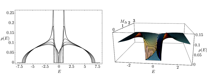
FIG. 5.: Density of states $\rho(E)=-\frac{1}{\pi}\mathrm{Re}G^{R}(E)$ with different values of $M_{\Delta}$. On the left side, the gap is reduced and finally closed as $M_{\Delta}$ runs through $M_{\Delta}=(0.01,\;0.1,\;0.5,\;1,\;1.6,\;2)$. The figure on the right side gives an overview for $0.2<M_{\Delta}<3.0$.

IX Competition between superconductivity and spin glass order

This section is devoted to the solution of the replica symmetric equations presented for the coexistence problem in section V. The phase diagram does not depend strongly on quantum–dynamical corrections $\chi(\omega)-\chi(0)$, where $\chi(0)=\beta(\tilde{q}-q)$, which are small for small $\Delta$ and small ratios $t/J$. The full problem is probably harder to solve than the infinite–dimensional Hubbard model. Thus approximations are necessary at present. One may view the superconducting order parameter like a generalized transverse field which induces a quantum-dynamical spin glass. If one has in mind the analysis of quantum phase transitions and the zero temperature limit in particular, then it is important to study the dynamic mean field theory similarly to the way it was done in Ref. [20] or in Refs. [19] and [21] for the Ginzburg Landau theory.
In turn it was mentioned that the existing dynamic theories may not be able to keep track of nonperturbative phenomena, mentioning the Griffith singularities as a possible source of concern [19].
Thus it is worthwhile to study thoroughly the already difficult spin/charge–static mean field theory.
The phase diagram illustrated in Figures 6 and 7 is obtained from the free energy of model ${\cal{H}}_{Jv}$. Saddle point solutions $q$, $\tilde{q}$, and $\Delta$ are found from the coupled selfconsistent equations given above. The physical solutions of these coupled equations are not easy to identify. Even outside the SG-phase multiple solutions exist and changeovers of stability occur as chemical potential $\mu$, temperature T, or interaction ratio $v/J$ are varied. This leads to the complexity of the phase diagram displayed in Figures 6 and 7.

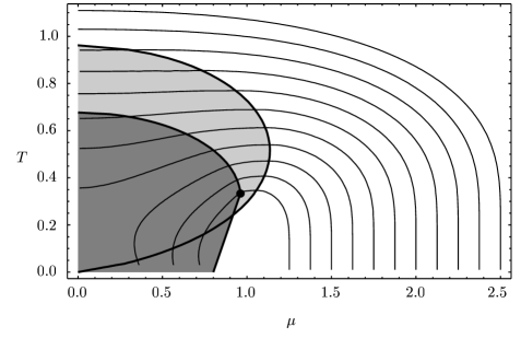
FIG. 6.: Phase diagram of competing spin glass (SG) and superconducting (SC)-transitions (thin lines) for various attractive couplings $v$ (given by $v=2J\mu_{e.p.}$ at lines’ right endpoint ($T=0,\mu=\mu_{e.p.}$)), at fixed $J=1$, and as a function of chemical potential $\mu$ (dark grey area: maximum SG-domain for $v=0$). Thin lines enclose SC-phases, which remove pieces of the ($v=0$) SG-phase or suppress it totally at large enough $v/J$. The bold line delimiting the light grey area joins tricritical points ($T_{c}$-maxima) on SC-critical curves and encloses 1st order transitions on its left

Figures 6 and 7 reveal unique features of the competition between SG- and SC-order. For example, an enhanced fermion concentration $\nu(\mu)$ reduces the effective spin density at larger $|\mu|$ and is seen to suppress the spin glass phase stronger than it eliminates the superconducting one as $\nu(\mu)\rightarrow$ 0 or 2. Within a large region above the SG-phase, the SC-critical curves become deformed, as Fig.6 shows for $v/J<4.5$, due to the increasing spin glass fluctuations feeded by the random magnetic interaction.
As the critical SC-curve passes through a maximum and starts to descend with decreasing $\mu$, the SC-transitions change from second to first order. For still smaller ratios $v/J$ the SC-line enters the $v=0$ SG-phase: in this case, magnetic moments freeze first and a discontinuous SG-SC transition follows at lower temperature (shown for $v/J=3.25,3.5,3.75$). For still smaller $v/J$ the 1st order SC-line falls rapidly to zero and the SG-phase prevents superconducting order up to a critical value $\mu_{c}$. The replica symmetric solution leaves open the possibility of reentrant SC - SG transitions, as one can observe for $v/J=2.5,2.75,3$ in Figure 6.
(remark: if one prefers to include a factor $\frac{1}{2}$ into the definition of the spin operators (we chose $\hat{\sigma}^{z}\equiv n_{\uparrow}-n_{\downarrow}$, $\hbar=1$) a factor of $\frac{1}{4}$ would rescale the ratios $v/J$ given throughout this paper.)

FIG. 7.: Phase diagram close to the spin glass transition (bold line: pure SG-transition, bold-dashed line: paramagnetic stability limit) showing the stability limits of the superconducting (SC) phase (dotted horizontal lines, given only for $v/J=3.5,3.0$) and of the non-SC phase (dashed thin lines) bifurcating at SC-tricritical points. SC-critical (continued thin) lines are shown down to small $v/J$.

Figure 7 complements Figure 6 by adding, within a magnification of the SG-SC boundary, the stability limits of the superconductor; it also displays second order SC-transition lines crawling into the phase separation regime of the Ising spin glass for small $v/J$ and $T$. For $T\rightarrow 0$, the Quantum Parisi Phase must be expected, which means that the paramagnetic stability limit and the thermodynamic transition shift to smaller $\mu$. The increase of SG-energy due to replica symmetry breaking (RPSB), also known from the standard model [24], is evaluated for the fermionic model in the final chapters. Lacking sufficient information on the full Parisi solution we employ for the moment numerical solutions of fermionic TAP-equations [34, 30] to arrive at a straight line estimate of the discontinuous paramagnet-SG transition curve. Discontinuous SC-SG transitions for $\frac{v}{J}<2.5$ must occur in between this curve and the SC-SG transition at $\frac{v}{J}=2.5$. It is currently not possible to locate better the position of these discontinuous transitions at low $T$. This would require to unite the dynamic mean field theory with the Parisi solution at infinite RPSB and probably with Dotsenko–Mézard VRSB (despite the discontinuity, one step RPSB may yield a good approximation but it is not the exact solution at and near $T=0$). This remains an important research problem for the future.
Furthermore, we arrived at the following conclusions:
i) There is no coexistence of spin glass - and local pairing superconducting order parameter in zero magnetic field. The detailed analysis of the free energy and of all stability conditions shows only SC-SG transitions between $\{q\neq 0,\Delta=0\}$ and $\{q=0,\Delta\neq 0\}$ for $H=0$. We stress that this is concluded from our $O((t/J)^{0})$–calculations covering local pairing superconductivity in a magnetic band; our experience with metallic spin glasses [35, 21] tells us that small $t/J$ will not change the conclusion, but a large hopping band appearing as a nonmagnetic band, squeezed in between the two magnetic bands, may allow for the coexisting SC - SG order parameter. We believe that this interesting and difficult question is disconnected from the one where coexistence relies on a special symmetry like d–wave superconductivity.
ii) The transition between the two phases is always discontinuous and exists only within a certain range of chemical potentials $\mu$ (or filling $\nu$).
iii) For large enough $v/J$, like $v/J>4.13$ at half-filling for example, the spin glass is prevented by the superconducting transition, which is continuous for $v/J>4.55$ at half-filling; below this value it becomes discontinuous. The tricritical line, which separates these domains is included in Figure 6 for several values of $v/J$ and as a function of the chemical potential.
iv) Decreasing the temperature at fixed $\mu<.96$ (see Figure 6), a second transition from SG to superconductivity occurs at $T_{c}<T_{f}(v=0)$. Figures 6 and 7 display the exact numerical results of the replica symmetric theory. The spin glass free energy, increased by only a few percent at higher temperatures, rises substantially at smaller temperatures due to RPSB and thus enlarges the superconducting domain. Recalling that reentrant behaviour finally disappears at the spin glass-ferromagnetic boundary under $\infty$–step RPSB [15], the reentrance from superconductor to spin glass and back to the superconductor seems to disappear already at 1–step RPSB, since the SC-SG boundary will not become a vertical line in the $(T,\mu)$–plane (unlike boundaries between SG and (anti)ferromagnetic phases in the $(T,H)$–plane for magnetic models [15]).

FIG. 8.: Stable selfconsistent solutions (continuous lines) and unstable solutions (dashed lines) of the superconducting order parameter $\Delta$ for $v=3$ (with $J=1$) and $q=0$. Depending on the value of $\mu$, 4 regions are distinguished: below $\mu=0.955$, a locally stable solution with $\Delta\neq 0$ emerges at $T_{3}=0.475$, and there may or may not be a first order transition, depending on the free energies of the $\Delta=0$ and $\Delta>0$ solutions. For $0.955<\mu<1.14$, the $\Delta=0$ solution becomes unstable in a certain temperature range and a first order superconducting transition occurs. The second locally stable $\Delta=0$ solution at low tempatures always has a higher free energy, there is no second first order solution. For $1.14<\mu<\frac{1}{v}=1.5$ the transition is continuous and both $T_{c}$ and $\Delta(T=0)$ decrease with increasing $\mu$. For higher $\mu$ the superconducting phase disappears completely.

Figure 8 shows the effect of random magnetic fluctuations, described by $\tilde{q}(T,\mu)$, on the superconducting order parameter for characteristic values of $\mu$ and $v/J=3$, in order to explain the stability of the different phases and the competition between them. The absence of coexistent order parameters allows to set $q=0$.
In a magnetic field new aspects arise: the transition temperature of the superconductor will be reduced and finally vanish for $H>H_{c2}$, leaving a smeared spin glass transition for sufficiently small $\mu$. The overlap parameter $q$ is nonzero in a field and then coexists with $\Delta$, since the field can penetrate the present type II superconductor. Thus the Almeida Thouless line can enter the superconductor, infiltrating ergodicity breaking there.
We analyze the superconducting phase by means of the Green’s functions: we derive the normal one ${\cal{G}}(\epsilon_{n})$ , the anomalous one ${\cal{F}}(\epsilon_{n})$, and relevant particle-hole-$\Pi_{ph}(\omega_{m})$ and particle-particle bubble diagrams $\Pi_{pp}(\omega_{m})$ for various limits. Superconductivity arising in the magnetic band much larger than the hopping band is described by

$${\cal{G}}(\epsilon_{l})= \sum_{\zeta=\pm\sqrt{|\Delta|^{2}+\mu^{2}}}\frac{1}{\tilde{q}(\exp(\beta^{2}\tilde{q}/2)+\cosh(\beta\zeta))}\frac{\zeta+\mu}{\zeta}\Bigl{(}\frac{1}{4}\cosh(\beta\zeta)(i\epsilon_{l}-\zeta)\hskip 2.84544pt{\cal{U}}\left[1,\frac{3}{2},\frac{-(\zeta-i\epsilon_{l})^{2}}{2\tilde{q}}\right]$$ (36)

$$+\frac{1}{8}\sum_{s=\pm 1}(i\epsilon_{l}-\zeta-s\beta\tilde{q})e^{\beta^{2}\tilde{q}/2}\hskip 2.84544pt{\cal{U}}\left[1,\frac{3}{2},\frac{-(\zeta-i\epsilon_{l}+s\beta\tilde{q})^{2}}{2\tilde{q}}\right]\Bigr{)}$$ (37)

$${\cal{F}}(\epsilon_{l})= \sum_{\zeta=\pm\sqrt{|\Delta|^{2}+\mu^{2}}}\frac{\Delta}{\tilde{q}(\exp(\beta^{2}\tilde{q}/2)+\cosh(\beta\zeta))}\frac{1}{\zeta}\Bigl{(}\frac{1}{4}\cosh(\beta\zeta)(i\epsilon_{l}-\zeta)\hskip 2.84544pt{\cal{U}}\left[1,\frac{3}{2},\frac{-(\zeta-i\epsilon_{l})^{2}}{2\tilde{q}}\right]$$ (38)

$$+\frac{1}{8}\sum_{s=\pm 1}(i\epsilon_{l}-\zeta-s\beta\tilde{q})e^{\beta^{2}\tilde{q}/2}\hskip 2.84544pt{\cal{U}}\left[1,\frac{3}{2},\frac{-(\zeta-i\epsilon_{l}+s\beta\tilde{q})^{2}}{2\tilde{q}}\right]\Bigr{)}$$ (39)

Here, $\mathcal{U}$ denotes the hypergeometric $\mathcal{U}$-function (Kummer function)[36]. Note that the branch cut on the real axis separating the regimes of retarded and advanced Green’s functions is a feature of the Hypergeometric $\mathcal{U}$-function. The SC order parameter obeys $\Delta=vT\sum_{\epsilon}{\cal{F}}(\epsilon)$.

FIG. 9.: Density of states $\rho(E)$ and ${\rm{Re}}(F(E))$, for ($v=5J,\mu=0,T_{c}\approx 1.11J$) and real energies $E$, show crossover from strongly to weakly gapless superconductivity for decreasing temperatures $T/J=1.1,1.0,.9,.8$ and $.7$, labeling $\rho$ from top to bottom at $E=0$ and ${\rm{Re}}(F)$ vice versa.

The solution for ${\cal{G}}(\epsilon)$ provides (after analytical continuation) the density of states $\rho(E)$, $E\equiv\epsilon+\mu$. A typical result is plotted together with Re$(F)$ in Figure 9. Weak fermion hopping–effects and dynamic corrections from $\Pi_{ph}(\omega)$ and $\chi(\omega)$ are negligible here. In principle the frustrated magnetic interaction interferes by means of a Lorentzian–shaped dynamic susceptibility, which becomes however $\delta$-like weighted at zero frequency as $\Delta\rightarrow 0$. Thus near the phase boundary, where we wish to represent the pairbreaking effects of the spin glass fluctuations competing with superconducting order, the given exact solutions of the $Q$–static model remain sufficiently good approximations. While the dynamic problem cannot be solved exactly, the given zero-frequency solution provides a starting point for a new dynamic approximation which we’ll present in a future publication.
The plots of Figure 9 employ the stable selfconsistent solutions for $\tilde{q}(T,\mu)$ and $\Delta(T,\mu)$ inserted in the (analytic continuation) of solutions given by Eqs.(39) and (37). They demonstrate the crossover from strongly gapless superconductivity near the spin glass transition to a pronounced pseudogap deeper in the sc–phase. Although invisibly small for temperatures lower than roughly 20% below $T_{c}$, the density of states remains nonzero in the pseudogap regime and vanishes there only at $T=0$. In the strict sense of the word the superconductor is gapless for all temperatures. But after a transient shell near the magnetic phase boundary is crossed, the superconducting gap is almost perfect. One should remark that near the phase boundary, within the shell where the magnetic susceptibility is not yet strongly depressed, a piece of the smooth depletion of density of states is also of magnetic origin. It is not the spin glass gap, but the frustrated interaction tends to deplete DoS around the Fermi level and at the same time removes the sharp gap edges which would otherwise appear at all temperatures below the superconducting transition.
The rounding of the superconducting gap edges and its soft progression below $T_{c}$ is reminiscent of the magnetic gap found below spin glass transitions [14] but is of totally different origin.
Up to now we did not include corrections from the hopping assumed to be very weak. Fermion hopping of course introduces dynamic effects, and both the Q–static approximation as well as the quantum–dynamic one had been worked out before. The smallness of these effects of order $O(t/J)$ does not change the phase diagram derived for $t/J=0$. One may calculate peturbatively corrections as done in Ref. [35]. We refrained from doing this because it is only important for the quantum phase transition, which requires however the full Parisi solution and the analysis of vector replica symmetry breaking as discussed before.
As one starts to look deeper into the superconducting phase, the magnetic band narrows however and eventually the fermion hopping (bandwidth) starts to dominate. Then, the normal and the anomalous Green’s function cross over into the hopping band solution given by Eqs.(24) and (25), respectively. The transition temperature derived from these solutions illustrates in Figure 10 the crossover from linear Bose condensation $T_{c}(v)$-dependence to exponential BCS-type superconductivity.

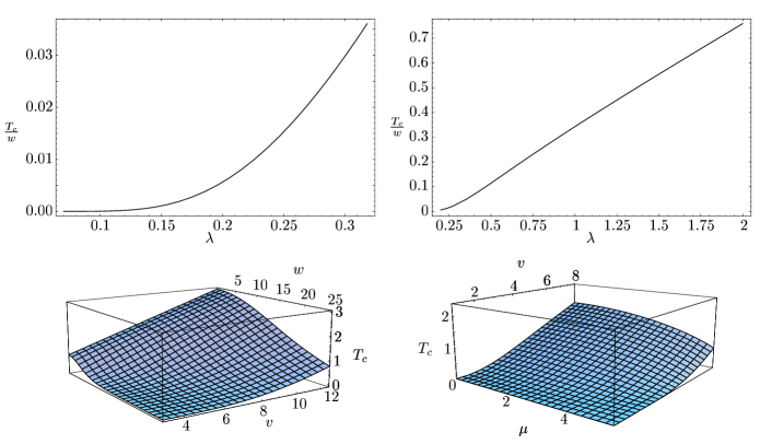
FIG. 10.: upper left: BCS–type exponential decay for small couplings $\lambda\equiv v\rho_{F}$; upper right: linear Bose condensation type $T_{c}(\lambda)$–regime; lower left: Complete crossover from Bose condensation type to BCS behaviour illustrated in 3D plot of $T_{c}(v)$ as the attractive coupling versus hopping bandwidth ratio $v/w$ decreases; lower right: BCS–Bose crossover also displayed as a function of chemical potential $\mu$

The Bose-BCS crossover can be followed through the whole parameter range due to the local property of the one-particle Green’s functions, a feature appreciated as well in the $d=\infty$ method for clean systems [37, 38]. The suppression of one particle phase coherence, due to infinite dimensions in clean systems or by symmetry requirement in the quenched average used here, results in type II superconductivity with the two particle coherence length replacing the standard one in the Ginzburg Landau theory (many details including paramagnetic pairbreaking were published in Ref. [39]). The puzzling coexistence phenomena in zero field, manifested by the absence of stable $(q\neq 0,\Delta\neq 0)$-solutions and by nonexisting common onset of magnetic and superconducting order on one hand and coexistence within phase separation regimes on the other, is further elucidated by the bubble diagram $\Pi_{pp}(T,\omega)$. The critical condition $1=v\Pi_{pp}(T_{c},\omega=0)$ can only be satisfied for $v>v_{min}$, with $v_{min}=4.14J$ at half filling. One can solve for $T_{c}=T_{f}$, finding $v=4.186J$ at half filling for example, but the second solution at $T_{c}^{\prime}>T_{c}$ for this coupling $v$ turns out to be the stable one. The thermodynamic transition occurs at a still higher temperature $T_{c1}>T_{c}^{\prime}$. Thus the calculation based on the two-particle Green’s functions confirms the absence of simultaneous and continuous onset of spin glass and superconducting order.
For the sake of transparency we discussed only fully frustrated magnetic interactions and zero field phenomena. Subsequent antiferromagnetic-spin glass-superconductor transitions, as $\mu$ increases are not simply obtained once $J_{ij}$ contains an antiferromagnetic part. A model extension by the Hubbard interaction can change this; allowance for different symmetries of the order parameter, and the dynamic quantum Parisi phase are further examples for future research on links between antiferromagnetism, spin glass order, and superconductivity.
The model we analyzed here proved to have a characteristic crossover between strongly and weakly gapless superconductivity, due to correlations induced by the frustrated magnetic interaction and depending on the vicinity of a spin glass phase.

X Effects of replica permutation symmetry breaking on the spin glass - superconductor phase boundary

Despite the absence of coexisting order parameters, the phase boundary depends on replica symmetry breaking due to the change of the spin glass free energy. This change becomes important at low temperatures. There, the increase in free energy entrained by RPSB becomes large enough to suppress reentrant behaviour. In Figure 11 the free energies are shown for $\mu=0.1$ and for a moderately large attractive coupling $v=3.5$: the left upper corner shows the increasing deviation and enhancement of the free energy with 1RPSB. The clearly visible crossing between the SC-curve and the spin glass curve indicates the thermodynamic discontinuous phase transition from spin glass in the intermediate temperature while the SG - PM transition is shown where the corresponding (and almost indistinguishable on the given scale) free energies become equal. Another example is given in the following Figure 12 for $\mu=0.3$.

FIG. 11.: Free energies $f$ of the disordered and spin glass solutions, together with the superconducting solution for $v=3.5$. It is easy to infer the SC–SG first order transition. At the second order transition SG–PM, the free energies of the spin–glass and the disordered solutions merge. Note that the disordered solution is unstable with respect to $q$ below this transition, therefore it is not the physical one although it has the lowest free energy. Also clearly visible is the difference between the 1–step RSB solution and the replica–symmetric one. It becomes important at low temperatures.

The consequences of 1RPSB–corrections on the phase diagram as shown in these figures are quite clear. As the free energies exceed substantially the replica-symmetric ones in the low temperature regime, where reentrance was observable in 0RPSB, the 1RSB–corrections strongly suppress reentrance. A first indication of this is shown in Figure 13.

FIG. 12.: Free energies $f$ of the disordered, spin glass, and superconducting solutions as in Fig. 11, for $\mu=0.3$ and $v=3.0$. Here one sees clearly how the SG-SC first order transition is affected by RPSB. Also, reentrance from SC to SG is suppressed with increasing RPSB, because the maximum of the SG solution becomes less pronounced and shifts to lower temperatures. For infinite RPSB we expect it to be at $T=0$.

FIG. 13.: Phase diagram including 1–step RPSB corrections to the phase diagram of Figure 6. Crosses indicate points of the SG–SC boundary calculated in 1–step RPSB. The deviations from the RS–calculations are most significant for low temperatures and suppress reentrant transitions.

The numerical effort in calculating 1RPSB results at very low temperatures is high and we shall report elsewhere a more detailed analysis employing a more dense set of chemical potentials.
For a certain set of chemical potentials we also calculated the fermion filling factor as a function of temperature as shown in Figure 14 for 1–step RPSB. The turnaround at low temperatures into a filling which decreases as the temperature increases from zero may belong to the unstable regime below the AT–instability–line, while the dots are 1step–RPSB results taken from the crossover line $\partial^{2}F/\partial\tilde{q}^{2}=0$. The curve shown for $\mu=.1$ and any other curve with $\mu<.119$ lies entirely in the stable regime at 1–step RPSB, but this changes with the order $k$ of RPSB, since the gap decreases to zero [7] as $k\rightarrow\infty$.

FIG. 14.: The fermion concentration $\nu(\mu)$ in 1–step RPSB as a function of temperature, shown for chemical potentials $\mu=.6,.5,...,.1$ from top to bottom. Dots indicate the location of the random field crossover line.

XI Discussion, outlook, open problems

A Expectations on lower dimensional corrections: which mean field predictions are robust?

Dimensional dependences can lead to inapplicability of mean field theories to lower-dimensional systems in a way similar to the failure of numerical results on too small systems.
While correlation functions explore phase transitions with high sensitivity and thus depend strongly on dimensions, particularly as those drop below their upper or lower critical values, there are less sensitive quantities like energies depending much less on these complications. Only their derivatives are more or less sensitive. Also gaps of excitation spectra which are related to the competition of different scales, can be rather robust.

B A comparison with the gap structure of the twodimensional periodic Anderson model

The spin glass generated charge gap of the fermionic Ising spin glass has been shown to have important consequences and we considered a gap digged out by coexisting magnetic and superconducting gap (despite noncoexistence in zero magnetic field). We find remarkable the fact that the gap structure obtained for either a fictitious or a finite-field-driven coexistence of spin glass order and superconductivity on one hand is comparable with the gap structure of the twodimensional periodic Anderson model [40]. The latter was derived by the Quantum Monte Carlo method for a twodimensional model. Clearly the mixed valence coupling corresponds to our superconducting order parameter in the role as a gap generator. One may pick two arbitrary values of $q$ and $\Delta$, not necessarily selfconsistent, to match the gap structure seen by Vékic et al [40] for the PAM model. We stress once more that this is not derived selfconsistently and its interest lies in the gap structure enabled by the functional dependence of the present model, the possibility to match a twodimensional systems gap structure by the present mean field theory, and the possibility that a magnetic field may realize the structure.
So we observe several models with rather high analogies: The periodic Anderson model, where the competition between the magnetic moment quenching Kondo effect and the RKKY interaction is important, its disordered version, which also falls into the class of randomly interacting models, the present SG - SC competition in a magnetic band model, and its smeared three band version. The relation between these models deserves further analysis. We shall invent for this purpose a technique which allows to treat dynamic interaction effects properly.

C Hopping band: the effective three-band Ising spin glass

We considered the limit of a magnetic band large compared to the fermion hopping band. This parameter range refers to transitions between a very bad conductor and superconductivity which stems from pairing in the magnetic band(s). We discussed in detail the frustrated magnetic interaction being at the origin of these magnetic bands, and their decay deep in the superconducting phase as well. Since the interesting parameter range for competition between spin glass and superconductivity requires the corresponding interactions $J$ and $v$ to be roughly of the same order, and since we deliberately restricted the analysis to very small $t/J$, the Bose condensation type of superconductivity was considered. Competition between spin glass and BCS–type superconductivity - within the same theory - can be investigated under the condition of a large hopping band. This refers to a nonmagnetic third band occupying essentially the space evacuated by spin glass order between the two magnetic bands; strong dynamic effects emerge and many important features may become different from the one described here: Theories for effects of comparable fermion hopping in metallic spin glasses exist [21, 35], but the coexistence with BCS-type superconductivity is an open question, since pairing may occur in the nonmagnetic band. The strong overlap with the magnetic bands sustaining spin glass order does however not seem to allow for an intuitive prediction on the fate of order parameter coexistence.

XII Acknowledgements

This research was supported by the Deutsche Forschungsgemeinschaft under research project Op28/5–1 and by the SFB410. One of us (H.F.) also wishes to acknowledge support by the Villigst foundation. We are grateful for discussions with J.A. Mydosh, B. Rosenow, and F. Steglich.

REFERENCES

- [1] J. A. Mydosh, J. Magn. Magn. Mat. 157/158, 606 (1996).
- [2] H. Spille et al., J. Magn. Magn. Mat. 76/77, 539 (1988).
- [3] S. Barth et al., J. Magn. Magn. Mat. 76/77, 455 (1988).
- [4] F. C. Chou et al., Phys. Rev. Lett. 75, 2204 (1995).
- [5] I. Korenblit, V. Cherepanov, A. Aharony, and O. E. Wohlmann, cond-mat/9709056 (1997).
- [6] D. J. Scalapino, Phys. Rep. 250, 329 (1995).
- [7] R. Oppermann and B. Rosenow, Europhys. Lett. 41, 525 (1998).
- [8] M. J. Nass, K. Levin, and G. S. Grest, Phys. Rev. B 23, 1111 (1981).
- [9] A. Sengupta and A. Georges, Phys. Rev B 52, 10295 (1995).
- [10] S. G. Magalhaes and A. Theumann, cond-mat/9810366 (1998), we found this work after completion of ours, cond-mat/9809001; the work by Theumann et al contains only a simple result at half–filling and moreover does not take care of replica symmetry breaking.
- [11] K. H. Fischer and J. Hertz, Spin Glasses (Cambridge University Press, Cambridge, 1991).
- [12] W. Brenig, Phys. Rep. 251, 153 (1995).
- [13] L. Balents, M. Fisher, and C. Nayak, cond-mat/9803086 (1998).
- [14] R. Oppermann and B. Rosenow, Phys. Rev. Lett. 80, 4767 (1998).
- [15] K. Binder and A. Young, Rev. Mod. Phys 58, 801 (1986).
- [16] F. J. Wegner, Phys. Rev. B 19, 783 (1979).
- [17] H. Rieger and A. Young, Phys. Rev. B 53, 8486 (1996).
- [18] H. Rieger and A. Young, Phys. Rev. B 54, 3328 (1996).
- [19] N. Read, S. Sachdev, and J. Ye, Phys. Rev B 52, 384 (1995).
- [20] Y. V. Fedorov and E. F. Shender, JETP Lett. 43, 681 (1986).
- [21] S. Sachdev, N. Read, and R. Oppermann, Phys. Rev B 52, 10286 (1995).
- [22] G. Büttner and K. D. Usadel, Phys. Rev B 41, 428 (1990).
- [23] B. Rosenow and R. Oppermann, Phys. Rev. Lett. 77, 1608 (1996).
- [24] G. Parisi, J. Phys. A 13, 1887 (1980).
- [25] E. J. S. Lage and J. R. L. de Almeida, J. Phys. C: Solid State Phys. 15, L1187 (1982).
- [26] P. Mottishaw and D. Sherrington, J. Phys. C: Solid State Phys. 18, 5201 (1985).
- [27] J. de Almeida and D. Thouless, J. Phys. A 11, 983 (1978).
- [28] F. A. da Costa, C. S. O. Yokoi, and S. R. A. Salinas, J. Phys. A 27, 3365 (1994).
- [29] V. Dotsenko and M. Mézard, J. Phys. A 30, 3363 (1997).
- [30] M. Rehker and R. Oppermann, cond-mat/9806092 (1998), to be published in J. Phys.: Condens. Matter.
- [31] R. Oppermann, Z. Phys. B 63, 33 (1986).
- [32] A. Altland and M. Zirnbauer, Phys. Rev B 55, 1142 (1997).
- [33] S. Schohe, R. Oppermann, and W. Hanke, Z. Phys. B 83, 31 (1991).
- [34] D. Thouless, P. Anderson, and R. Palmer, Phil. Mag. 35, 593 (1977).
- [35] R. Oppermann and M. Binderberger, Ann. Physik 3, 494 (1994).
- [36] M. Abramovitz and I. Stegun, Handbook of Mathematical Functions (Dover Publ. Inc, NY, 1972).
- [37] D. Vollhardt, in Correlated electron systems, edited by V. J. Emery (World Scientific, Singapore, 1992).
- [38] A. Georges, G. Kotliar, W. Krauth, and M. Rozenberg, Rev. Mod. Phys. 68, 13 (1996).
- [39] R. Oppermann, Physica A 167, 301 (1990).
- [40] M. Vékic et al., Phys. Rev. Lett. 74, 2367 (1995).