Effect of band filling in the Kondo lattice: A mean-field approach

Abstract

The usual Kondo-lattice, including an antiferromagnetic exchange interaction between nearest-neighboring localized spins, is treated here in a mean-field scheme that introduces two mean-field parameters: one associated with the local Kondo effect, and the other related to the magnetic correlations between localized spins. Phases with short-range magnetic correlations or coexistence between those and the Kondo effect are obtained. By varying the number of electrons in the conduction band, we notice that the Kondo effect tends to be suppressed away from half filling, while magnetic correlations can survive if the Heisenberg coupling is strong enough. An enhanced linear coefficient of the specific heat is obtained at low temperatures in the metallic state.

I Introduction

The denomination Kondo lattice[1] applies to systems which are characterized by a lattice of localized magnetic moments coexisting with a conduction band. Examples are found among Cerium compounds, such as CeAl₃, CeCu₆, CeCu₂Si₂, etc.,[2] as well as some Uranium or other rare-earth compounds.[1] At high temperatures, the localized moments behave essentially as independent impurities, similarly to what happens in dilute alloys. At low temperatures, a coherent heavy-fermion behavior is observed where the system resembles a Fermi-liquid with enhanced values of parameters such as the specific-heat constant $\gamma$ and the magnetic susceptibility $\chi$. This is a scenario found in the Cerium compounds mentioned above. However, deviations from this behavior are observed: some systems can show a magnetically ordered ground state, as happens, for example, in CeAl₂, CeB₆, and CePd₂Al₃, or become superconducting at low temperatures, as is the case of CeCu₂Si₂,[3, 4] CeCu₂Ge₂ at high pressures,[5] and some Uranium compounds like UPt₃,[6] UBe₁₃,[7] and URu₂Si₂,[8] among others. Besides that, neutron-scattering experiments[9, 10, 11, 12] point to the presence of strong short-range magnetic correlations in CeCu₆, CeInCu₂, and CeRu₂Si₂, for which a Fermi-liquid ground state is stable, but that are probably close to the conditions for a magnetic instability.

This coexistence of magnetic correlations and Kondo effect was recently discussed by Iglesias, Lacroix, and Coqblin[13] within a mean-field approach that has points in common with a slave-boson treatment by Coleman and Andrei.[14] Their analysis was restricted to the case of a half-filled conduction band, which is of relevance for Kondo insulators.[15] The role played by the conduction-band filling is obviously very important for metallic compounds that show heavy-fermion behavior, and to the discussion of underscreened systems.[16]

In this paper we study the effect of band filling in the stability of the Kondo state and short-range magnetic correlations in the Kondo lattice using a mean-field approach closely related to the one employed in Ref. [13]. Two mean-field parameters are introduced, in connection with the local correlations generated by the Kondo effect, and the non-local ones that indicate tendency towards magnetic order. These quantities behave as order parameters of thermodynamic phases where one of them or both are non-zero, while both vanish in the high-temperature “normal” phase. Besides the order parameters themselves, we calculate the free energy, the specific heat, and the single-particle density of states. We focus on the changes observed when one moves away from half-filling, as well as the competition between correlations induced by the Kondo coupling and those produced by a Heisenberg exchange term added to the original Kondo-lattice model. When this interaction is strong, the system first develops magnetic correlations, and only at a lower critical temperature does the Kondo effect appear, depleting but not suppressing the existing correlations. In contrast, when the Heisenberg interaction is small compared to the local Kondo coupling, the latter dominates, giving rise to a single phase where magnetic correlations are mostly induced by the Kondo effect, and can even change sign when the band filling is low enough. The specific heat that we obtain in the metallic case shows an enhanced linear coefficient, indicating that important qualitative aspects of the physics of heavy-fermion systems are retained in the mean-field approach.

In Sec. II we introduce the model Hamiltonian and the fermionic representation of localized moments. In Sec. III we choose the relevant fields in terms of which we rewrite the Hamiltonian, perform the mean-field decoupling, find the energy eigenvalues, and introduce self-consistency equations for the mean-field parameters, as well as relations to obtain the physical quantities of interest. Our results are presented in Sec. IV, and a critical discussion of them appears in Sec. V.

II Model Hamiltonian

The usual Kondo-lattice Hamiltonian is

$$H=\sum_{{\bf k}\sigma}\varepsilon_{\bf k}n^{c}_{{\bf k}\sigma}-J_{\text{K}}\sum_{i}{\bf s}_{i}\cdot{\bf S}_{i}\>,$$ (1)

where ${\bf s}_{i}$ stands for the total conduction-electron spin at lattice site $i$, ${\bf S}_{i}$ is the spin operator associated to the localized moments, and the first term in the right-hand side describes the conduction band in usual notation. We choose spin-1/2 localized moments, assigning them to “$f$ electrons”. We also add a Heisenberg-like interaction between nearest-neighbor localized spins. The Kondo-lattice Hamiltonian then reads

$$H = \sum_{{\bf k}\sigma}\varepsilon_{\bf k}n^{c}_{{\bf k}\sigma}+E_{0}\sum_{i}n^{f}_{i\sigma}$$ (3)

$$\mbox{}-J_{\text{K}}\sum_{i}{\bf s}_{i}\cdot{\bf S}_{i}-J_{\text{H}}\sum_{\langle ij\rangle}{\bf S}_{i}\cdot{\bf S}_{j}\,,$$

The term with the factor $E_{0}$ is just a constant provided that we remain in the subspace of unit occupation number for the $f$ electrons at every site, which is the constraint that ensures the equivalence of Eqs. (1) and (3) if the exchange interaction is also included in the original model.

The spin operators are rewritten in the usual fermionic representation

$$s_{i}^{z}=\frac{1}{2}\left(n^{c}_{i\uparrow}-n^{c}_{i\downarrow}\right)\>, \qquad S_{i}^{z}=\frac{1}{2}\left(n^{f}_{i\uparrow}-n^{f}_{i\downarrow}\right)\>,$$ (4)

$$s_{i}^{+}=c_{i\uparrow}^{\dagger}c_{i\downarrow}\>, \qquad S_{i}^{+}=f_{i\uparrow}^{\dagger}f_{i\downarrow}\>,$$ (5)

$$s_{i}^{-}=c_{i\downarrow}^{\dagger}c_{i\uparrow}\>, \qquad S_{i}^{-}=f_{i\downarrow}^{\dagger}f_{i\uparrow}\>.$$ (6)

There is no unique way of rewriting the Hamiltonian in terms of fermion operators. For instance, the terms involving the $z$ component of the spins can be left as in Eq. (4), or the number operators can be explicitly written as products of creation and annihilation operators, whose ordering can then be altered using the fermionic anticommutation relations. The final choice of form to write down these terms will actually depend on the mean-field decoupling that will be employed, as we will discuss in the next section.

III Mean-field scheme

The first step in constructing the mean-field Hamiltonian is to choose the relevant fields. The original Hamiltonian is naturally written in terms of spin fields. However, if we just introduced a mean-field decoupling of spin products we would end up with a magnetic Hamiltonian. Since we intend to describe the Kondo effect as well, we have to choose fields that couple $c$ and $f$ electrons at the same site, since these will tend to form local singlets. We can also couple $f$ electrons from neighboring sites in order to describe the short-range magnetic correlations that will develop between the localized moments. A convenient way to do this is to define the (Hermitian) fields

$$\hat{\lambda}_{i\sigma} \equiv \frac{1}{2}\left(c_{i\sigma}^{\dagger}f_{i\sigma}+f_{i\sigma}^{\dagger}c_{i\sigma}\right)\>,$$ (7)

$$\hat{\Gamma}_{ij\sigma} \equiv \frac{1}{2}\left(f_{i\sigma}^{\dagger}f_{j\sigma}+f_{j\sigma}^{\dagger}f_{i\sigma}\right)\>,$$ (9)

where $\sigma$ labels the spin orientation (up or down) with respect to the $z$ axis, and $i$ and $j$ are nearest-neighbor sites in the definition of $\hat{\Gamma}_{ij\sigma}$. It is straightforward to write down the contributions of transversal spin components in terms of these fields. We have

$$s_{i}^{x}S_{i}^{x}+s_{i}^{y}S_{i}^{y} = -\sum_{\sigma}\hat{\lambda}_{i\sigma}\hat{\lambda}_{i,-\sigma}\>,$$ (10)

$$S_{i}^{x}S_{j}^{x}+S_{i}^{y}S_{j}^{y} = -\sum_{\sigma}\hat{\Gamma}_{ij\sigma}\hat{\Gamma}_{ij,-\sigma}\>,$$ (12)

where we have made explicit usage of the constraint $n_{i}^{f}=1$. Products involving the $z$ component of the spins are slightly more complicated to deal with, and sometimes these are decoupled as spin fields.[13] However, this breaks the spin symmetry, and results in the stability of a magnetic state, with total suppression of the Kondo effect, unless the local average magnetic moment is forced to be zero. Hence, we will avoid this procedure, using the same kind of representation for all spin components. After some algebraic manipulations, we obtain

$$s_{i}^{z}S_{i}^{z} = \frac{1}{4}\left(n_{i}^{c}+n_{i}^{f}\right)-\frac{1}{4}n_{i}^{c}n_{i}^{f}-\sum_{\sigma}\hat{\lambda}^{2}_{i\sigma}\>,$$ (13)

$$S_{i}^{z}S_{j}^{z} = \frac{1}{4}\left(n_{i}^{f}+n_{j}^{f}\right)-\frac{1}{4}n_{i}^{f}n_{j}^{f}-\sum_{\sigma}\hat{\Gamma}^{2}_{ij\sigma}\>.$$ (15)

Due to the constraint $n_{i}^{f}=1$ at all sites, the terms containing number operators in Eqs. (13) will yield a constant shift of the energies (after summation over the lattice sites). This terms can then be dropped, leaving the Kondo and Heisenberg parts of the Hamiltonian respectively written as

$$H_{\text{K}}=J_{\text{K}}\sum_{i\sigma}\left(\hat{\lambda}_{i\sigma}+\hat{\lambda}_{i,-\sigma}\right)\hat{\lambda}_{i\sigma}\>,$$ (16)

and

$$H_{\text{H}}=J_{\text{H}}\sum_{\langle ij\rangle\sigma}\left(\hat{\Gamma}_{ij\sigma}+\hat{\Gamma}_{ij,-\sigma}\right)\hat{\Gamma}_{ij\sigma}\>.$$ (17)

We now proceed with a standard mean-field decoupling of the operator products in these Hamiltonians, introducing the mean-fields $\lambda_{i\sigma}\equiv\langle\hat{\lambda}_{i\sigma}\rangle$ and $\Gamma_{ij\sigma}\equiv\langle\hat{\Gamma}_{ij\sigma}\rangle$. From Eqs. (16) and (17) ones sees that each field couples with a spin-independent quantity. Thus, there will be no breakdown of spin symmetry, i. e., no magnetic states. Taking this into account, together with translational invariance, we can simplify the notation, using $\lambda_{i\sigma}\equiv\lambda$ and $\Gamma_{ij\sigma}\equiv\Gamma$.

We are now in a position to put all contributions together: the noninteracting terms of Eq. (3) and the mean-field versions of the interaction Hamiltonians (16) and (17). Reverting to the fermionic representation, and adding a chemical potential $\mu$ for the conduction electrons, we can write the complete mean-field Hamiltonian

$$H^{\text{MF}} = \sum_{{\bf k}\sigma}(\varepsilon_{\bf k}-\mu)n^{c}_{{\bf k}\sigma}+E_{0}\sum_{i}n^{f}_{i\sigma}$$ (20)

$$\mbox{}+2J_{\text{K}}\lambda\sum_{i\sigma}\left(c_{i\sigma}^{\dagger}f_{i\sigma}+f_{i\sigma}^{\dagger}c_{i\sigma}\right)+\bar{E}_{\text{K}}$$

$$\mbox{}+2J_{\text{H}}\Gamma\sum_{\langle ij\rangle\sigma}\left(f_{i\sigma}^{\dagger}f_{j\sigma}+f_{j\sigma}^{\dagger}f_{i\sigma}\right)+\bar{E}_{\text{H}}\>,$$

with

$$\bar{E}_{\text{K}}=-4NJ_{\text{K}}\lambda^{2}\>,\quad\bar{E}_{\text{H}}=-2zNJ_{\text{H}}\Gamma^{2}\>,$$ (21)

where $z$ represents the coordination number of a site in the lattice, and $N$ is the total number of sites.

We will choose the conduction band to be a tight-binding band of width $2W$ (with nearest-neighbor hopping only) in a (hyper)cubic lattice in $d$ dimensions, so that we can write

$$\varepsilon_{\bf k}=-\frac{W}{d}\sum_{\mu}\cos(k_{\mu}a)\>,$$ (22)

where $\mu$ labels the wavevector components, and $a$ is the lattice parameter. With this choice, the term with $J_{\text{H}}$ in Eq. (20) will have the same ${\bf k}$-dependence as the conduction band, except for the band width. We see, thus, that the mean-field decoupling introduces a non-zero band width to the $f$ electrons. At this point, we have to replace the constraint $n_{i}^{f}=1$ with the much weaker constraint $\langle n_{i}^{f}\rangle=1$. Hence, the virtual charge fluctuations introduced by the fermion representation of the localized spins have been “put in the mass shell” by the mean-field decoupling. Of course, this real charge fluctuations are spurious, but the method relies on the expectation that the physics of the system will be reasonably preserved on the phase-space surface where the constraint $\langle n_{i}^{f}\rangle=1$ holds. In order to improve on this point one would have to envisage better ways to take into account the constraint of single occupancy on the $f$ levels at each site.

Leaving aside, for the moment, the constant terms ${E}_{\text{K}}$ and ${E}_{\text{H}}$, the Hamiltonian (20) is easily diagonalized, yielding the energy eigenvalues[13]

$$E_{\bf k}^{\pm} = \frac{1}{2}\bigg{[}\,\varepsilon_{\bf k}(1+B)+E_{0}-\mu$$ (24)

$$\mbox{~{}}\pm\sqrt{\left[\varepsilon_{\bf k}(1-B)-E_{0}-\mu\right]^{2}+16J_{\text{K}}^{2}\lambda^{2}}\;\bigg{]}\>,$$

where $B\equiv-4dJ_{\text{H}}\Gamma/W$. These energies are spin-degenerate, as we remarked before. With them and the corresponding eigenvectors we can compute any average of relevant physical quantities in the system. The chemical potential $\mu$ is determined by the equality $\langle n_{\bf k}^{c}\rangle=n$, where $n$ is the (chosen) density of conduction electrons. $E_{0}$ plays the role of a chemical potential for the $f$ electrons, being fixed by the condition $\langle n_{\bf k}^{f}\rangle=1$. The mean-field parameters $\lambda$ and $\Gamma$ are determined through the selfconsistency equations

$$\lambda = \frac{1}{2N}\sum_{\bf k}\left\langle c_{{\bf k}\sigma}^{\dagger}f_{{\bf k}\sigma}+f_{{\bf k}\sigma}^{\dagger}c_{{\bf k}\sigma}\right\rangle\>,$$ (25)

$$\Gamma = -\frac{1}{WN}\sum_{\bf k}\varepsilon_{\bf k}\langle n^{f}_{{\bf k}\sigma}\rangle\>.$$ (27)

We also check the self-consistency process by evaluating the free-energy, which can be written as

$$F = -2T\sum_{{\bf k},\alpha=\pm}\log\left[1+e^{-E_{\bf k}^{\alpha}/T}\right]$$ (29)

$$\mbox{}+\bar{E}_{\text{K}}+\bar{E}_{\text{H}}-(E_{0}-\mu n)N\>.$$

where $T$ is the temperature (in energy units). Finally, we can calculate the average internal energy

$$E=2\sum_{{\bf k},\alpha=\pm}E_{\bf k}^{\alpha}f(E_{\bf k}^{\alpha})+\bar{E}_{\text{K}}+\bar{E}_{\text{H}}-(E_{0}-\mu n)N\>,$$ (30)

where $f(\varepsilon)$ stands for the Fermi function. The last term in Eqs. (29) and (30) is needed to compensate for the fact that $\mu$ and $E_{0}$ are already included in the Hamiltonian. The specific heat can now be obtained as $c_{V}=\partial E/\partial T$, and we can check for an enhanced linear coefficient $\gamma$, which is a signature of heavy-fermion behavior.

IV Results

In order to be close to real systems, we considered a three-dimensional simple-cubic lattice ($z=6$). However, given that all wave-vector dependence occurs through $\varepsilon_{\bf k}$, we turn all ${\bf k}$ sums into integrals over the conduction-band energies, for which we use a semi-elliptical density of states of the form

$${\cal D}(\varepsilon)=\left\{\begin{array}[]{lc}\frac{3}{4}(1-\varepsilon^{2})\;,&-1\leq\varepsilon\leq 1\>;\\ 0\>,&\mbox{otherwise}\>.\end{array}\right.$$ (31)

Here we have set $W=1$, so that all energies are measured in units of the half band width. We choose both $J_{\text{K}}$ and $J_{\text{H}}$ to be negative, which corresponds to the usual Kondo coupling, and antiferromagnetic Heisenberg interactions between nearest-neighboring localized spins. The latter would be naturally interpreted as generated by a superexchange mechanism, and could also mimic the RKKY interaction in the mean-field Hamiltonian, although this is a debatable issue: we will see below that there exist induced spin correlations due to the Kondo coupling alone, and these are more closely related to the RKKY mechanism.

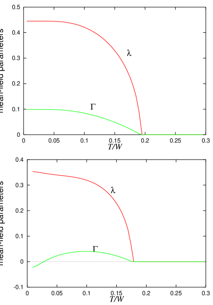
FIG. 1.: Mean-field parameters $\lambda$ and $\Gamma$ as functions of temperature for $n=1$ (top) and $n=0.6$ (bottom), in the case where the Heisenberg interaction is small compared to the Kondo coupling: $J_{\text{K}}/W=-0.5$, $J_{\text{H}}/W=-0.1$.

After numerically solving the set of self-consistency equations, we find that both $\lambda$ and $\Gamma$ behave as typical mean-field order parameters, which vanish at high temperatures, and become non-zero through second-order phase transitions at well defined critical temperatures. We identify the region where $\lambda\neq 0$ with the Kondo regime, and the corresponding critical temperature is interpreted as the Kondo temperature ($T_{\text{K}}$) for the lattice. We call $T_{\text{Corr}}$ the temperature below which short-range magnetic correlations appear ($\Gamma\neq 0$). When $|J_{\text{H}}|<<|J_{\text{K}}|$, both transitions occur at the same temperature, while $|J_{\text{H}}|$ comparable to or larger than $|J_{\rm K}|$ gives $T_{\text{Corr}}>T_{\text{K}}$, as obtained earlier for the half-filled case.[13] We show a typical example of this behavior in Figs. 1 and 2, where we compare the results for a half-filled and a less-than-half-filled conduction band. (Due to particle-hole symmetry, the results are actually symmetric around $n=1$.)

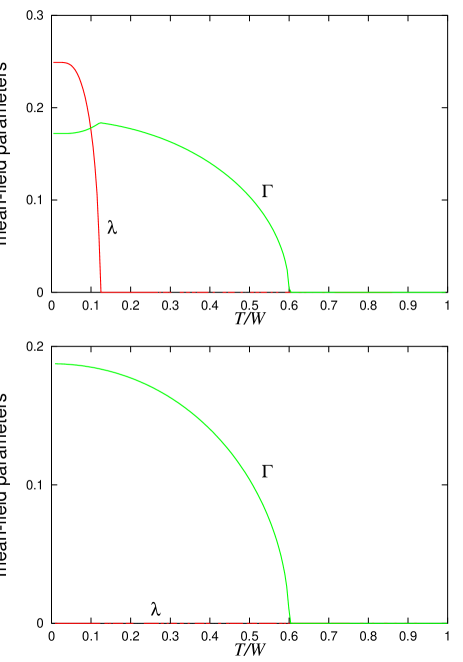
FIG. 2.: Same as in Fig. 1, but with a large Heisenberg interaction: $J_{\text{K}}/W=-0.5$, $J_{\text{H}}/W=-1.0$.

Departure from the half-filled situation causes a reduction of the critical temperatures, except for $T_{\text{Corr}}$ in the large-$|J_{\text{H}}|$ regime. Although the sign of $\Gamma$ does not have a direct physical meaning, since spin correlations are related to the square of the operator associated to $\Gamma$ according to Eq. (13), we believe that the change of sign observed in Fig. 1 for the case of low band filling indicates that the nearest-neighboring spin correlations have become ferromagnetic, as expected in this limit. This is only observed at low temperatures, where the Kondo effect is large, and the induced part of the correlations dominate. In contrast, close to $T_{\text{K}}$, $\lambda$ is small, and the antiferromagnetic correlations due to the Heisenberg interaction dominate. In order to check this, we would have to calculate the average $\langle{\hat{\Gamma}}_{ij\sigma}^{2}\rangle$ that appears in the spin-spin correlations, Eq. (13). Unfortunately, this is related to averages of products of number operators in each site, which are non-trivial in spite of the non-interacting nature of the effective Hamiltonian. More specifically, these products involve number operators at displaced wavevectors, which prevents the transformation of momentum summations into energy integrals. Notice, however, that when $\Gamma$ goes to zero, spins in different sites become decoupled in the mean-field Hamiltonian. Then, their correlations go to zero, which should happen when they change from antiferro- to ferromagnetic.

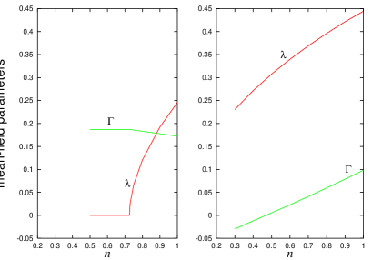
FIG. 3.: Variation of the mean-field parameters with band filling at fixed temperature ($T/W=0.05$). In the left panel we have dominant magnetic correlations ($J_{\text{K}}/W=-0.5$, $J_{\text{H}}/W=-1.0$), while in the right panel the Kondo effect dominates ($J_{\text{K}}/W=-0.5$, $J_{\text{H}}/W=-0.1$).

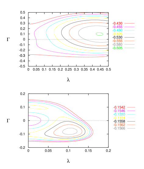
FIG. 4.: Equal free-energy contours at $n=1$ (top) and $n=0.1$ (bottom) for $|J_{\text{H}}|$ small, showing the complex topolgy that arises at low filling. The values of the free energy for each contour, quoted on the right, are in units of the half band width.

In Fig. 3 we plot the mean-field parameters as functions of the band filling for a fixed (low) temperature (T/W=0.05). For large $|J_{\text{H}}|$ (left panel), the Heisenberg coupling dominates, keeping $\Gamma$ almost unchanged, while $\lambda$ is strongly reduced as we move away from $n=1$, since we have an underscreening situation. This picture is completely changed in the small-$|J_{\text{H}}|$ regime (right panel). Now both parameters are reduced as one moves away from half-filling. One sees that $\Gamma$ is now equally sensitive to $n$, which suggests that in this regime the part of the inter-site correlations induced by the conduction electrons is dominant. It eventually yields ferromagnetic spin correlations, as discussed above. We checked that a similar behavior is observed if we fix $J_{\text{H}}=0$, when all spin correlations are induced by the conduction electrons.

We have cut the curves in the right panel of Fig. 3 for small $n$ because the convergence of our numerical calculations, which involve iterating the set of self-consistency equations for the mean-field parameters and occupation numbers, becomes very delicate in that region. In order to see what is happening, we evaluate the free energy $F$ [Eq. (29)] for fixed $\lambda$, $\Gamma$, $n$, and $T$, adjusting only $\mu$ and $E_{0}$. Typical contour plots of $F$ at low temperature as a function of $\lambda$ and $\Gamma$, for half-filling and for $n$ very small, in the small-$|J_{\text{H}}|$ regime, are shown in Fig. 4. We can see that the minimum at finite $\lambda$ and $\Gamma$ that exists at half-filling is displaced towards small values of $\lambda$ and negative values of $\Gamma$ as $n$ is reduced. Eventually, a new minimum appears for $\Gamma>0$, since the energy eigenvalues, Eq. (24), are symmetric with respect to the sign of $\Gamma$ when $\lambda=0$. Thus, when $\lambda$ approaches zero (as $n$ is reduced) we have two shallow minima separated by a very broad and low maximum at $\lambda=\Gamma=0$, which causes problems to the numerical iteration of the self-consistency equations since distant points in the $\lambda$-$\Gamma$ space are very close in free-energy.

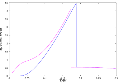
FIG. 5.: Variation of the specific heat (per unit cell) with temperature for $n=1$ (continuous) and $n=0.6$ (dashed), when the Heisenberg interaction is weak ($J_{\text{K}}/W=-0.5$, $J_{\text{H}}/W=-0.1$). Notice the insulating and metallic behavior at low temperatures in each case, and the lambda-shaped transition at the point where both the Kondo effect and magnetic correlations disappear.

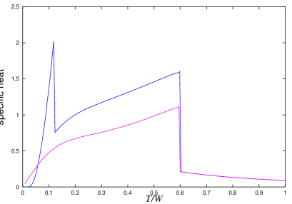
FIG. 6.: Same as in Fig. 5, but for strong Heisenberg coupling ($J_{\text{K}}/W=-0.5$, $J_{\text{H}}/W=-1.0$), showing the transitions at different temperatures.

Our results for the specific heat as a function of temperature are presented in Figs. 5 and 6. The phase transitions appear in the usual “lambda shape” characteristic of mean-field approximations. There are two jumps in the case of large $|J_{\text{H}}|$, at the temperatures where the Kondo effect and the magnetic correlations disappear. These points coincide when $|J_{\text{H}}|$ is small. We can also see the existence of a gap at the Fermi level for the half-filled band, yielding an exponentially vanishing specific heat for $T\to 0$. In contrast, away from half-filling one sees a linear regime at low temperatures. The linear coefficient obtained for $n=0.6$, $|J_{\text{K}}|=0.5$, and $|J_{\text{H}}|=0.01$ is $\gamma\sim 10\gamma_{0}$, where $\gamma_{0}$ is the corresponding value in the absence of interactions. We have, thus, some enhancement of $\gamma$, although the true heavy-fermion limit ($\gamma\sim 10^{2}\gamma_{0}$) is not reached. Such an enhancement should correspond to a high density of states (DOS) at the Fermi level. We calculated the DOS as

$$\rho(\omega)=-\frac{1}{\pi}\sum_{\alpha=\pm}\sum_{{\bf k}\sigma}{\rm Im}\,G_{{\bf k}\sigma}^{\alpha}(\omega+i0^{+})\>,$$ (32)

in terms of the one-particle Green’s functions

$$G_{{\bf k}\sigma}^{\alpha}(z)=\frac{1}{z-E_{\bf k}^{\alpha}}\>.$$ (33)

The DOS depends on temperature through $\lambda$ and $\Gamma$, which appear in the energies $E_{\bf k}^{\alpha}$. We plot the low-temperature DOS in Fig. 7, for both $n=1$ and $n=0.6$, in the small-$|J_{\text{H}}|$ regime. We can see that the Fermi level ($\omega=0)$ falls in the gap for $n=1$, while it is located at a point corresponding to a very high density of states away from half filling. The gap that is observed immediately above the Fermi level in the latter case explains the reduction (or at least levelling off) of the specific heat just above the linear region in Fig. 5. As the temperature is increased, the gap in the DOS as well as the peaks around it are narrowed until a superposition of a free conduction band and a localized $f$-level is recovered above $T_{\text{K}}$.

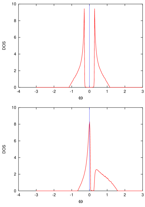
FIG. 7.: Total single-particle density of states at $T/W=0.01$, for $n=1$ (top) and $n=0.6$ (bottom), with $J_{\text{K}}/W=-0.5$, $J_{\text{H}}/W=-0.1$. The frequencies are measured in units of $W$. Notice that the Fermi level (vertical dashed line) lies in the gap at half-filling, and inside a high peak for $n<1$.

V Conclusions

We have presented here a detailed mean-field analysis of the Kondo lattice, emphasizing the effects of conduction-band filling in the properties of the system. The regime where the Kondo effect is observed, and the one in which short-range magnetic correlations are present appear as thermodynamic phases with well defined critical temperatures. These phases are characterized by non-zero values of the mean-field parameters associated to local correlations between localized and conduction electrons ($\lambda$), and between localized electrons on nearest-neighboring sites ($\Gamma$). We find a regime in which the Kondo effect and short-range magnetic correlations coexist, in agrrement with experimental observations in some Ce compounds.[9, 10, 11, 12] The main consequence of changing the electronic density in the conduction band with respect to half-filling is a tendency to suppress the Kondo effect. Magnetic correlations are equally suppressed if a direct Heisenberg interaction between nearest-neighboring localized spins is weak, while they are almost insensitive to the band filling for strong Heisenberg interactions. In the latter case the critical temperatures for the two order parameters are different, and one notices a partial suppression of magnetic correlations in the region where the Kondo effect is observed. The phase transitions appear as lambda-shaped peaks in the specific heat, which also shows an enhanced linear coefficient in the metallic situation ($n\neq 1$), corresponding to an enhanced density of states at the Fermi level.

To a good extent, the physics of Kondo systems is recovered here, at least qualitatively, both for insulators ($n=1$) and conductors ($n\neq 1$). A weak point of this treatment is the impossibility to describe magnetically ordered states. Here one would have to go back to the choice of relevant fields, trying to write down a Hamiltonian in which both Kondo and spin fields were present before the mean-field decoupling. It would be interesting to improve the method along these lines without loosing its formal simplicity. This simplicity constitutes the main quality of this approach, allowing evaluation of many relevant physical quantities in an unrestricted range of parameters and conditions, and yielding qualitative understanding of the behavior of the system as a whole.

- [1] A. C. Hewson, The Kondo Problem to Heavy Fermions, Cambridge University Press (1992).
- [2] B. Coqblin, J. Arispe, J. R. Iglesias, C. Lacroix, and Karyn Le Hur, J. Phys. Soc. Japan 65, Suppl. B, 64 (1995).
- [3] F. Steglich, J. Aarts, C. D. Bredl, W. Lieke, D. Meschede, W. Franz, and H. Schafer, Phys. Rev. Lett. 43, 1892 (1979).
- [4] F. G. Aliev, N. B. Brandt, R. V. Lutsiv, V. V. Moshchalkov, and S. M. Chudinov, JETP Lett. 35, 539 (1982).
- [5] E. Vargoz and D. Jaccard, J. Magn. Magn. Mater. 177-181, 294 (1998).
- [6] G. R. Stewart, Z. Fisk, J. O. Willis, and J. L. Smith, Phys. Rev. Lett. 52, 679 (1984).
- [7] H. R. Ott, H. Rudigier, Z. Fisk, and J. L. Smith, Phys. Rev. Lett. 50, 1595 (1983).
- [8] T. T. Palstra, A. A. Menovsky, J. van der Berg, A. J. Dirkmaat, P. H. Kes, G. J. Nieuwenhuys, and M. A. Mydosh, Phys. Rev. Lett. 55, 2727 (1985).
- [9] J. Rossat-Mignot, L. P. Regnault, J. L. Jacoud, C. Vettier, P. Lejay, J. Flouquet, E. Walker, D. Jaccard, and A. Amato, J. Magn. Magn. Mater. 76-77, 376 (1988).
- [10] L. P. Regnault, W. A. C. Erkelens, J. Rossat-Mignot, P. Lejay, and J. Flouquet, Phys. Rev. B 38, 4481 (1988).
- [11] J. Pierre, P. Haen, C. Vettier, and S. Pujol, Physica B 163, 463 (1990).
- [12] H. v. Löhneysen, S. Mock, A. Neubert, T. Pietrus, A. Rosh, A. Schröder, O. Stockert, and U. Tutsch, J. Magn. Magn. Mater. 177-181, 12 (1998).
- [13] J. R. Iglesias, C. Lacroix, and B. Coqblin, Phys. Rev. B 56, 11820 (1997).
- [14] P. Coleman and N. Andrei, J. Phys.: Condens. Matter 1, 4057 (1989).
- [15] M. A. Continentino, Phys. Lett. A 197, 417 (1995).
- [16] P. Nozières and A. Blandin, J. Physique 41, 193 (1980).