Impurity corrections to the thermodynamics in spin chains using a transfer-matrix DMRG method

Abstract

We use the density matrix renormalization group (DMRG) for transfer matrices to numerically calculate impurity corrections to thermodynamic properties. The method is applied to two impurity models in the spin-1/2 chain, namely a weak link in the chain and an external impurity spin. The numerical analysis confirms the field theory calculations and gives new results for the crossover behavior.

I Introduction

The study of quantum impurities remains a large part of condensed matter physics. The Kondo effect is maybe one of the most famous examples for impurity effects, but more recently much effort has been devoted to impurities in low-dimensional magnetic systems in connection with high temperature superconductivity[2]. For the particular case of impurities in quasi one-dimensional systems, much progress has been made with field theory descriptions e.g. for the Kondo model[3], quantum wires[4], and spin chains[5]. In those cases, the impurity behaves effectively as a boundary condition at low temperatures and the behavior can be described in terms of a renormalization crossover between fixed points as a function of temperature[3].

Numerically this renormalization picture has been confirmed[5, 6, 7], but so far it was only possible to examine a limited number of energy eigenvalues in the spectrum. While some efforts have been made to extract thermodynamic properties from the energy spectrum directly[8], such an approach is tedious and remains limited by finite system sizes. Monte Carlo simulations appear to be well suited for determining thermodynamic properties, but for the particular case of impurity properties it turns out to be difficult to accurately determine a correction which is of order $1/N$, where $N$ is the system size. We now apply the transfer matrix DMRG to impurity systems. This overcomes those problems by explicitly taking the thermodynamic limit $N\to\infty$, while still being able to probe impurity corrections and local properties at finite temperatures even for frustrated systems (which are not suitable for Monte Carlo simulations due to the minus sign problem).

There are two separate impurity effects that we wish to address. The first is the impurity correction $F_{\rm imp}$ to the total free energy of a one dimensional system

$$F_{\rm imp}\ =\ \lim_{N\to\infty}(F_{\rm total}-NF_{\rm pure}),$$ (1)

where $F_{\rm pure}$ is the free energy per site for an infinite system without impurities. In other words, the impurity contribution is that part of the total free energy that does not scale with the system size $N$

$$F_{\rm total}=NF_{\rm pure}+F_{\rm imp}+{\cal O}(1/N).$$ (2)

Therefore, the impurity free energy $F_{\rm imp}$ is directly proportional to the impurity density of the system, and it immediately determines the corresponding impurity specific heat and impurity susceptibility, i.e. quantities that can be measured by experiments as a function of temperature and impurity density. Despite the obvious importance of this impurity contribution we are not aware of any numerical studies that considered this quantity for any non-integrable impurity system. Traditional methods would require an extensive finite size scaling analysis to track down the $1/N$ correction to the total free energy per site, but our approach allows us to calculate $F_{\rm imp}$ directly in the thermodynamic limit. We would like to point out that in other studies the response of an impurity spin to a local magnetic field is often termed “impurity susceptibility”, but we prefer to reserve this expression for the impurity contribution

$$\chi_{\rm imp}=-\frac{\partial^{2}}{\partial B^{2}}{F_{\rm imp}},$$ (3)

where $B$ is a global magnetic field on the total system.

The second aspect of impurity effects are local properties of individual sites near the impurity location, e.g. correlation functions and the response to a local magnetic field. Local properties have been the central part of a number of works for many impurity models[6, 7, 8, 9, 10, 11]. Our approach is now able to calculate these impurity effects directly in the thermodynamic limit and we get quick and accurate results to extremely low temperatures. It turns out that the local impurity effects can be determined much more accurately and to lower temperatures than the impurity contribution $F_{\rm imp}$, which remains limited by accuracy problems even with this method.

The Density Matrix Renormalization Group (DMRG)[12] has had a tremendous success in describing low energy static properties of many one-dimensional (1D) quantum systems such as spin chains and electron systems. More recently many useful extensions to the DMRG have been developed. Nishino showed how to successfully apply the density matrix idea to two-dimensional (2D) classical systems by determining the largest eigenvalue of a transfer matrix[13]. Bursill, Xiang and Gehring have then shown that the same idea can be used to calculate thermodynamic properties of the quantum spin-1/2 $XY$-chain[14]. The method has later been improved by Wang and Xiang[15] as well as Shibata[16] and been applied to the anisotropic spin-1/2 Heisenberg chain with great success. In this paper we apply a generalization of the method to impurity systems, which is presented in section II. In Section III we study two different impurity models in the spin-1/2 chain and are able to confirm predictions from field theory calculations. Section IV concludes this work with a discussion of the results and a critical analysis of accuracy and applicability to other systems.

II The Method

The method of the transfer matrix DMRG can in principle be applied to any one-dimensional system for which a transfer matrix can be defined. As a concrete example we will consider the antiferromagnetic spin-1/2 chain, since this model is well understood in terms of field theory treatments and has direct experimental relevance. The Heisenberg Hamiltonian can be written as

$$H=\sum_{i=1}^{N}h_{i},\;\;\;\;h_{i}=J_{i}\;{\bf S}_{i}\cdot{\bf S}_{i+1}+B_{i}\;S_{i}^{z},$$ (4)

where $J_{i}$ is the exchange coupling between sites $i$ and $i+1$, and $B_{i}$ is an external magnetic field in the $z$-direction at site $i$. Periodic boundary conditions, ${\bf S}_{N+1}\equiv{\bf S}_{1}$, are assumed. The partition function is defined by

$$Z=\mbox{tr}\;e^{-\beta H}=\mbox{tr}\;e^{-\beta(H_{o}+H_{e})},$$ (5)

where $\beta=\frac{1}{k_{B}T}$ and where we in the last step have partitioned $H$ into odd and even site terms,

$$H_{o}=\sum_{i=1}^{N/2}h_{2i-1},\;\;\;\;H_{e}=\sum_{i=1}^{N/2}h_{2i}.$$ (6)

A The transfer matrix method

The quantum transfer matrix for this system is defined as usual via the Trotter-Suzuki decomposition[17]

$$Z_{M}=\mbox{tr}\left(e^{-\frac{\beta H_{o}}{M}}e^{-\frac{\beta H_{e}}{M}}\right)^{M},$$ (7)

where $M$ is the Trotter number. This expression approximates the partition function up to an error of order $(\beta/M)^{2}$ and becomes exact in the limit $M\rightarrow\infty$. By inserting a complete set of states between each of the exponentials in Eq. (7) and rearranging the resulting matrix elements, the partition function can be written as a trace over a product of transfer matrices,[14]

$$Z_{M}=\mbox{tr}\;\prod_{i=1}^{N/2}{T}_{M}({2i-1}),$$ (8)

where ${T}_{M}({2i-1})$ is the $2^{2M}\times 2^{2M}$ dimensional quantum transfer matrix from lattice site $2i-1$ to site $2i+1$. Note that ${T}_{M}$ is in general not symmetric. However, if the two-site Hamiltonian $h_{2i-1}$ and $h_{2i}$ of Eq. (4) is invariant under the exchange $2i-1\leftrightarrow 2i$, and $2i\leftrightarrow 2i+1$ respectively, as is the case unless we have applied a non-uniform magnetic field, ${T}_{M}$ is a product of two symmetric transfer matrices, one from site $2i-1$ to site $2i$ and the other from site $2i$ to $2i+1$. For a uniform system, the transfer matrix is independent of lattice site, ${T}_{M}({2i-1})\equiv{T}_{M}$, and the partition function is then given by

$$Z_{M}=\mbox{tr}\;{T}_{M}^{N/2}.$$ (9)

In the thermodynamic limit of the uniform system, $Z_{M}$ is given by

$$\lim_{N\rightarrow\infty}Z_{M}=\lambda^{N/2},$$ (10)

where $\lambda$ is the largest eigenvalue of ${T}_{M}$.

The largest eigenvalue $\lambda$ can be found exactly only for small Trotter numbers $M$. As $M$ increases, the dimension of ${T}_{M}$ grows exponentially, and we have to use some approximation technique to find $\lambda$. Analogous to the case where the DMRG can be used to find a certain eigenstate of a Hamiltonian as the number of lattice sites increase, we can use the DMRG to find the largest eigenvalue of ${T}_{M}$ as the Trotter number $M$ increase. The strategy is thus to start with a system block, ${T}^{s}_{M/2}$, and an environment block, ${T}_{M/2}^{e}$, with a small $M$. The superblock transfer matrix, ${T}_{M}$, with Trotter number $M$, is constructed by “gluing” together the system block with the environment block. Periodic boundary conditions in the Trotter direction must be used. The reduced density matrix is constructed from the target state, i.e. the eigenstate of ${T}_{M}$ with largest eigenvalue. Since the transfer matrix is non-symmetric, the left and right eigenvectors will not be complex conjugates of each other.

A reduced density matrix for the system as part of the superblock can be constructed by taking a partial trace of $T_{M}^{N/2}$ over the environment degrees of freedom[15],

$$\rho=\frac{1}{Z_{M}}\mbox{tr}_{\rm env}T_{M}^{N/2}.$$ (11)

In the thermodynamic limit only the state with the largest eigenvalue will contribute,

$$\rho\stackrel{{\scriptstyle N\to\infty}}{{\longrightarrow}}\mbox{tr}_{\rm env}|\psi^{R}\rangle\langle\psi^{L}|,$$ (12)

where $|\psi^{R}\rangle$ and $\langle\psi^{L}|$ are the right and left eigenvectors of the superblock transfer matrix, $T_{M}$, corresponding to the largest eigenvalue, $\lambda$. The matrix elements are given by $\rho_{i^{\prime},i}=\sum_{j}\psi^{R}_{i^{\prime},j}\psi^{L}_{i,j}$ , where $i$ and $j$ label the degrees of freedom of the system and the environment respectively and the target states are given by $\langle\psi^{L}|=\sum_{i,j}\psi^{L}_{i,j}\langle i|\langle j|$ and $|\psi^{R}\rangle=\sum_{i,j}\psi^{R}_{i,j}|i\rangle|j\rangle$.

The left and right eigenvectors of the density matrix with the largest eigenvalues are then used to define the projection operators onto the truncated basis. After the first iterations we will keep $m$ states for the system and the environment and the superblock will be $4m^{2}$ dimensional. More details on the transfer matrix DMRG algorithm for quantum systems have been presented in Refs. [14, 15, 16].

Since $\rho$ is non-symmetric it is not obvious that the eigenvalues are real, but because $\rho$ represents a density matrix we expect it to be positive definite. However, because of numerical inaccuracies complex eigenvalues tend to appear in the course of iterations. This is usually connected to level crossings in the eigenvalue spectra of the density matrix as $M$ is increased. In addition, we also observe that just before the complex eigenvalues appear, multiplet symmetries in the eigenvalue spectrum of $\rho$ may split up (often due to “level repulsion” from lower lying states which were previously neglected). To overcome this problem it is important to keep all original symmetries (i.e. eigenvalue multiplets of $\rho$) even as $M$ increases. For that purpose it is often necessary to increase the number of states $m$ just before a multiplet tends to split up, which avoids the numerical error that leads to the symmetry breaking. In case of a level crossing of two multiplets that do not split up, complex eigenvalues may still appear and it is then possible to numerically transform the complex eigenstate pair into a real pair spanning the same space. Since the transformed real pair still is orthonormal to every other eigenvector, this transformation does not cause any troubles for later iterations. With this method the eigenvalues stay complex until the two levels have crossed and moved enough apart, at which point the eigenvalues become real again. The renormalization procedure is therefore not as straightforward as in ordinary DMRG runs, since it is essential to track all eigenvalues of $\rho$ and to dynamically adjust the number of states $m$, thereby sometimes repeating previous iteration steps.

B Impurities and local properties

The renormalization scheme also allows the calculation of thermal expectation values of local operators. The magnetization of the spin at site $i$ is determined by

$$\langle S_{i}^{z}\rangle=\frac{1}{Z}\;\mbox{tr}\;S_{i}^{z}e^{-\beta H}.$$ (13)

The operator $S_{i}^{z}$ thus only has to be incorporated in the corresponding transfer matrix at site $i$. For the pure system, we then arrive at the formula[15]

$$\langle S_{i}^{z}\rangle=\frac{\langle\psi^{L}|{T}_{M}^{sz}(i)|\psi^{R}\rangle}{\lambda},$$ (14)

where ${T}_{M}^{sz}(i)$ is defined similar to ${T}_{M}(i)$ but with the additional operator $S^{z}_{i}$ included in addition to the Boltzmann weights. To measure the local bond energy, $h(i)={\bf S}_{i}\cdot{\bf S}_{i+1}$, a similar construction can be used.

Let us now assume that the system has a single impurity. The systems we will study is the periodic spin-1/2 chain with one weakened link or an external spin-1/2 coupled to one spin in the chain

$$H_{1} = H_{0}-\delta\!J\;{\bf S}_{N}\cdot{\bf S}_{1}$$ (15)

$$H_{2} = H_{0}+J^{\prime}\;{\bf S}_{1}\cdot{\bf S}_{f},$$ (16)

where

$$H_{0}=\sum_{i=1}^{N-1}J{\bf S}_{i}\cdot{\bf S}_{i+1}+J{\bf S}_{N}\cdot{\bf S}_{1}$$ (17)

is the periodic chain and ${\bf S}_{f}$ is the spin operator of an external spin-1/2. The models are depicted in Fig. 1.

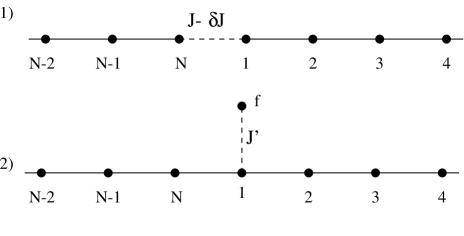
FIG. 1.: The impurity configurations considered in Eqs. (15) and (16). Note, that the left and right ends are joined with periodic boundary conditions.

For systems with such a local impurity, which is contained within two neighboring links, only one of the $T_{M}(i)$ in Eq. (8) will differ from a common $T_{M}$

$$Z_{M}=\mbox{tr}\;\left(T_{M}^{N/2-1}T_{\rm imp}\right),$$ (18)

where $T_{\rm imp}$ is the transfer matrix of the two links containing the impurity and $T_{M}$ is the transfer matrix describing the bulk. In the thermodynamic limit the partition function will still be dominated by the largest eigenvalue of the “pure” transfer matrix. From Eq. (18) we have

$$\lim_{N\rightarrow\infty}Z_{M}=\lambda^{N/2-1}\langle\psi^{L}|{T}_{\rm imp}|\psi^{R}\rangle,$$ (19)

where $\lambda$, $\langle\psi^{L}|$ and $|\psi^{R}\rangle$ all correspond to the pure system. The generalization of Eqs. (18) and (19) to impurity configurations ranging over more than two links is straightforward. In this case more than one impurity transfer matrix has to be introduced and this could be used to study e.g. multiple impurities and impurity-impurity interactions.

Let us define $\lambda_{\rm imp}\equiv\langle\psi^{L}|{T}_{\rm imp}|\psi^{R}\rangle$. The total free energy of the system is then given by

$$F = -\frac{1}{\beta}\ln Z$$ (20)

$$= -\frac{1}{\beta}\ln\left(\lambda^{N/2-1}\lambda_{\rm imp}\right)$$ (21)

$$= -\frac{N}{2\beta}\ln\lambda-\frac{1}{\beta}\ln\frac{\lambda_{\rm imp}}{\lambda}.$$ (22)

By comparing with Eq. (2) we can retrieve the pure and impure parts

$$F_{\rm pure}=-\frac{1}{2\beta}\ln\lambda,\;\;\;F_{\rm imp}=-\frac{1}{\beta}\ln\frac{\lambda_{\rm imp}}{\lambda}.$$ (23)

The impurity susceptibility can be found from the change of $F_{\rm imp}$ in a small magnetic field from Eq. (3)

$$\chi_{\rm imp}=-\frac{\partial^{2}}{\partial B^{2}}{F_{\rm imp}}.$$ (24)

Local properties such as the magnetization of the impurity spin can be determined by

$$\langle S_{\rm imp}^{z}\rangle=\frac{\langle\psi^{L}|{T}_{\rm imp}^{sz}|\psi^{R}\rangle}{\lambda_{\rm imp}}.$$ (25)

The magnetization of spins close to the impurity is readily obtained by

$$\langle S^{z}\rangle=\frac{\langle\psi^{L}|{T}_{M}^{sz}({T}_{M})^{x}{T}_{\rm imp}|\psi^{R}\rangle}{\lambda^{x+1}\;\lambda_{\rm imp}},$$ (26)

where $2x$ is the number of sites between the impurity and the spin of interest. Note that since a transfer matrix involves a total of three lattice sites, ${T}^{sz}_{M}$ can be constructed to measure the spin at any of these sites (or the mean value). The actual site of the measurement in Eq. (26) is thus determined both by $x$ and how ${T}^{sz}_{M}$ is set up. The expectation value in Eq. (26) is most easily calculated by first computing the vectors $\langle\psi^{L}|{T}_{M}^{sz}$ and ${T}_{\rm imp}|\psi^{R}\rangle$, then acting with ${T}_{M}$ on one of these states, and finally calculating the inner product of the resulting states. Eq. (26) can be generalized to measure any equal time correlation function with or without an impurity, e.g. by replacing ${T}_{\rm imp}$ by ${T}_{M}^{sz}$.

The reduced density matrix for the impurity system can be constructed by taking the thermodynamic limit of the impurity version of Eq. (11),

$$\rho=\frac{1}{Z_{M}}\mbox{tr}_{\rm env}\left(T_{M}^{N/2-1}T_{\rm imp}\right),$$ (27)

with $Z_{M}$ as in Eq. (18). In our calculations we have used the same density matrix as for the pure case, i.e. Eq. (12), and we have found it to give good results. This form can most easily be motivated by writing Eq. (27) on the form $\rho=\mbox{tr}_{\rm env}\left(T_{M}^{N/4-1}T_{\rm imp}T_{M}^{N/4}\right)/Z_{M}$. From a computational point of view, this method is also very convenient; by storing all target states and projection operators from the DMRG run for the pure system, all local impurities can be studied by simply using the same projection operators and target states. This makes subsequent DMRG runs for different impurity parameters very fast.

There are also other choices of density matrices that can be made. The thermodynamic limit of Eq. (27) can also be interpreted as $\rho\rightarrow|\psi^{R}\rangle\langle\psi^{L}|T_{\rm imp}/\lambda_{\rm imp}$ in which case the impurity transfer matrix would be taken into account in the density matrix. This would in some sense be analogous to including an operator different from the Hamiltonian in the density matrix of the ordinary “zero-temperature” DMRG, which is usually not necessary to measure e.g. correlation functions in the ordinary DMRG. This approach would destroy the computational advantage of using the pure density matrix, because the pure projection operators and target states could not be used but instead complete DMRG runs would have to be done for each impurity configuration and coupling.

III Results

A Field theory predictions

To make a meaningful analysis of the numerical results, we first need to understand the spin-1/2 chain in the framework of the quantum field theory treatment. This turns out to give a good description of the impurity behavior in terms of a renormalization flow between fixed points, and we will be able to set up concrete expectations for the impurity susceptibility in Eq. (3) as well as local properties.

The effective low energy spectrum of the spin-1/2 chain is well described by a free boson Hamiltonian density

$${\cal H}=\frac{v}{2}\left[(\Pi_{\phi})^{2}\,+\,({\partial_{x}\phi})^{2}\right],$$ (28)

plus a marginal irrelevant operator $\cos\sqrt{8\pi}\phi$ and other higher order operators which we have neglected. Here $\Pi_{\phi}$ is the momentum variable conjugate to $\phi$. In the long wave-length limit the spin operators can be expressed in terms of the bosonic fields using the notation of Ref. [5]

$$S^{z}_{j} \approx {1\over\sqrt{2\pi}}{\partial\phi\over\partial x}+(-1)^{j}\hbox{const.}\ \cos{\sqrt{2\pi}\phi}$$ (29)

$$S^{-}_{j} \approx e^{i\sqrt{2\pi}\tilde{\phi}}[\hbox{const.}\,\cos{\sqrt{2\pi}\phi}+(-1)^{j}\hbox{const.}],$$ (30)

At this point we can introduce the impurities in Eq. (15) and (16) in a straightforward way as perturbations. The field theoretical expressions for these perturbations can then be analyzed in terms of their leading scaling dimensions. Local perturbations with a scaling dimension of $d>1$ are considered irrelevant, while perturbations with a small scaling dimension $d<1$ are relevant and drive the system to a different fixed point. Hence, we can predict a systematic renormalization flow towards or away the corresponding fixed point, respectively.

Such an analysis has been made in Ref. [5] and the renormalization flows have been confirmed by determining the finite size corrections to the low energy spectrum[5]. In particular, a small weakening of one link in the chain

$$H_{1}=H_{0}-\delta\!J\;{\bf S}_{N}\cdot{\bf S}_{1}$$ (31)

has been found to be a relevant perturbation described by the operator $\sin\sqrt{2\pi}\phi$ with scaling dimension $d=1/2$, so that the periodic chain $(\delta\!J=0)$ is an unstable fixed point. The open chain $(\delta\!J=J)$ on the other hand is a stable fixed point where the perturbation is described by the leading irrelevant operator $\partial_{x}\phi(N)\partial_{x}\phi(0)$ with scaling dimension of $d=2$. Hence we expect a renormalization flow between the two fixed points as the temperature is lowered, and the temperature dependence of the impurity susceptibility as well as local properties will be described by a crossover function. Below a certain crossover temperature $T_{K}$ this crossover function describes the behavior of the stable fixed point (the open chain) while above $T_{K}$ the system may exhibit a completely different behavior. The crossover temperature $T_{K}$ itself is determined by the initial coupling strength $\delta\!J$

$$\lim_{\delta\!J\to 0}T_{K} \to 0$$ (32)

$$\lim_{\delta\!J\to J}T_{K} \to \infty.$$ (33)

In other words, close to the unstable fixed point the crossover temperature is very small, indicating that we have to go to extremely low temperatures before we can expect to observe the behavior of the stable fixed point.

A similar scenario holds for the impurity model with one external spin ${\bf S}_{f}$,

$$H_{2}=H_{0}+J^{\prime}\;{\bf S}_{1}\cdot{\bf S}_{f}.$$ (34)

In this case, the periodic chain $(J^{\prime}=0)$ is also the unstable fixed point, while the open chain with a decoupled singlet ($J^{\prime}\to\infty$) is the stable fixed point[5, 6].

As mentioned above, the renormalization flow has been confirmed for the energy corrections of individual eigenstates, but we now seek to extend this analysis to thermodynamic properties, which will allow us to determine the crossover behavior and $T_{K}$ directly.

B One weak link

Our first task is to establish the renormalization behavior from a periodic chain fixed point to the open chain fixed point as a function of temperature. To examine the effective boundary condition on the spin-operators, it is instructive to look at the correlation functions at spin-sites close to the impurity. For periodic boundary conditions, the leading operator for the spin $S^{z}_{1}$-operator is given by $\cos{\sqrt{2\pi}\phi}$ with scaling dimensions of $d=1/2$ according to Eq. (30). On the other hand, open boundary conditions restrict the allowed operators and the leading operator for $S^{z}_{1}$ is found to be $\partial_{x}\phi(0)$ with scaling dimension of $d=1$. Hence, the autocorrelation function at the impurity behaves differently, depending on the effective boundary condition

$$\langle S^{z}_{1}(\tau)S^{z}_{1}(0)\rangle\propto\left\{\begin{array}[]{lll}1/\tau&\phantom{nnn}&{\rm periodic\ b.c.}\\ 1/\tau^{2}&\phantom{nnn}&{\rm open\ b.c.}\end{array}\right.$$ (35)

Therefore, a useful quantity to consider is the response $\chi_{1}$ to a local magnetic field given by the Kubo formula

$$\chi_{1}(T) = \int^{1/T}\langle S^{z}_{1}(\tau)S^{z}_{1}(0)\rangle\,d\tau$$ (36)

$$\stackrel{{\scriptstyle T\to 0}}{{\longrightarrow}} \left\{\begin{array}[]{lll}-\log T&\phantom{nnn}&{\rm periodic\ b.c.}\\ {\rm const.}+{\cal O}(T)&\phantom{nnn}&{\rm open\ b.c.}\end{array}\right.$$ (39)

In Fig. 2 we have presented the results of $\chi_{1}$ for different impurity strengths $\delta\!J$ on a logarithmic temperature scale. For the periodic chain ($\delta\!J=0$) we clearly observe the logarithmic scaling, but for any finite $\delta\!J$ a turnover to a constant behavior is observed as $T\to 0$, i.e. the behavior of the open chain. The turnover temperature $T_{K}$ occurs at larger and larger values as we approach the stable fixed point [see Eq. (33)]. An interesting aspect is that the curves actually cross: At very high temperatures the high temperature expansion always dictates a larger response for a weakened link, while at very low temperatures this relation is reversed by quantum mechanical effects and the renormalization flow.

FIG. 2.: The local response $\chi_{1}$ of the spin ${\bf S}_{1}$ next to a weak link for different coupling strengths $\delta\!J/J=0,0.2,0.4,0.6,0.8,1$. The crossover to the open chain behavior occurs at different temperatures $T_{K}$ depending on the coupling strength.

We now turn to the true impurity susceptibility of Eq. (3) which is the experimentally more relevant quantity. Maybe the simplest non-trivial case to consider is the open chain $\delta\!J=J$. At low temperatures the impurity susceptibility can be calculated from the leading irrelevant local operator which is allowed in the Hamiltonian. This operator turns out to be $(\partial_{x}\phi(0))^{2}$ which gives a constant impurity susceptibility with a logarithmic correction similar to the pure susceptibility[18] as follows from a dimensional analysis. (In fact this operator can be absorbed in the free Hamiltonian by a defining a velocity $v$ that depends on the system size[19]. An explicit calculation of integrals over the correlation functions also comes to the same conclusion.)

$$\chi_{\rm imp}^{\rm open}(T)\ \stackrel{{\scriptstyle T\to 0}}{{\longrightarrow}}\ {\rm const.}+{\cal O}\left(1/\log(T/T_{0})\right)$$ (40)

While it is possible to calculate the impurity susceptibility numerically according to Eq. (23), the use of a second derivative in Eq. (24) causes large problems with the accuracy at lower temperatures since it involves taking the differences of large numbers. Luckily, the excess local susceptibility $\chi_{\rm local}$ of the first site under a global magnetic field turns out to give a good estimate of the true impurity susceptibility[11]

$$\chi_{\rm local}=\frac{d\langle S^{z}_{1}\rangle}{dB}-\chi_{\rm pure}\propto\chi_{\rm imp}+{\rm const.}$$ (41)

where $B$ is a global magnetic field and the constant is due to the alternating part[11]. The results for this quantity are shown in Fig. 3 which are consistent with Eq. (40). The second derivative in Eq. (24) has a similar behavior in the intermediate temperature range, but is not accurate enough to extrapolate to the $T\to 0$ limit as explained above.

FIG. 3.: The impurity susceptibility for an open chain, which is approximated by the excess susceptibility at an open end $\chi_{\rm local}$ (dots). At moderately low temperatures our data-fit (solid line) is consistent with the behavior in Eq. (40). The fit is $\chi_{\rm local}=1.895+18.6/\log(T/T_{0})$, with $\log(T_{0})=10$.

Now we are in the position to consider the impurity susceptibility of one weak link in the chain. By reducing $\delta\!J$ it is possible to tune the the system all the way from the open chain fixed point to the periodic chain. The operator $(\partial_{x}\phi(0))^{2}$, which was responsible for the open chain impurity susceptibility is thereby reduced continuously. However, it is an entirely different operator corresponding to ${\bf S}_{N}\cdot{\bf S}_{1}$ which is responsible for the renormalization. This operator changes scaling dimension as we go from periodic boundary conditions towards the open chain

$${\bf S}_{N}\cdot{\bf S}_{1}\propto\left\{\begin{array}[]{lll}\sin\sqrt{2\pi}\phi&d=1/2&{\rm periodic\ b.c.}\\ \partial_{x}\phi(N)\partial_{x}\phi(0)&d=2&{\rm open\ b.c.}\end{array}\right.$$ (42)

Since we wish to study the effect of this renormalization, we choose to subtract the open contribution systematically from $\chi_{\rm imp}$, so we obtain exactly the part which will exhibit the crossover of the renormalization

$$\chi_{\rm imp}(\delta\!J)-\delta\!J\ \chi_{\rm imp}^{\rm open}=f(T/T_{K})/T_{K}.$$ (43)

We see that this difference is zero at either fixed point. After subtracting $\delta\!J\chi_{\rm imp}^{\rm open}$ the impurity susceptibility comes only from the operator in Eq. (42), which allows us to postulate the scaling form in Eq. (43). Below $T_{K}$ the difference in Eq. (43) will asymptotically go to a constant for a very weak link $\delta\!J\sim J$, which comes from the $d=2$ operator in Eq. (42). Indeed we observe in Fig. 4 that this difference is negative and proportional to $J-\delta\!J\sim 1/T_{K}$ and largely temperature independent as $T\to 0$. On the other hand as $\delta\!J$ becomes small enough, the behavior is much different: The expression in Eq. (43) even decreases with $\delta\!J$ and the turn-over to constant behavior happens at much lower temperatures (outside the plot range).

FIG. 4.: The part of the impurity susceptibility which is attributed to the effects of the weakened link. For a very weak link $\delta\!J\sim J$ the magnitude increases linearly with $J-\delta\!J$ and saturates quickly, while the magnitude decreases again as we approach the periodic chain $\delta\!J\ll J$, but does not saturate as $T\to 0$.

Interestingly, this results in a highly nontrivial behavior as a function of $T$ and $T_{K}$ close to the unstable fixed point

$$\lim_{T\to 0}\lim_{T_{K}\to 0}f(T/T_{K})/T_{K} \propto T_{K}/T^{2}\ \propto\ \delta\!J^{2}\to 0$$ (44)

$$\lim_{T_{K}\to 0}\lim_{T\to 0}f(T/T_{K})/T_{K} \propto 1/T_{K}\ \propto\ 1/\delta\!J^{2}\to-\infty.$$ (45)

This means that at $T=0$ a minute perturbation $\delta\!J$ results in an extremely large negative $\chi_{\rm imp}\propto 1/\delta\!J^{2}$ (although this behavior occurs in an “unphysical” limit). The reason that the two limits do not commute is of course because one describes the behavior of the stable fixed point $T\ll T_{K}$, while the other one describes the behavior at the unstable fixed point. While our numerical results cannot show the entire crossover of Eq. (43), the increase below $T_{K}$ for small $J-\delta\!J$ is clearly observed as well as the decrease and change of curvature above $T_{K}$ for small $\delta\!J$. Therefore, our data in Fig. 4 supports the renormalization scenario and the nontrivial behavior of Eq. (45).

C One external spin

The model of an external spin antiferromagnetically coupled to the chain in Eq. (16) is maybe a little more exotic, but is still of great interest in a number of studies[5, 6, 7, 8, 9, 10, 20]. In Ref. [5] it was first shown that the stable fixed point corresponds to open boundary conditions with a decoupled singlet. This was confirmed numerically[7], but more recently Dr. Liu postulated a completely different behavior using some non-local transformations on Fermion-fields which mysteriously were rearranged to form a solvable model[20]. While we cannot trust or understand many of his calculations, the predictions are in strong contrast to any previous expectations and should be tested explicitly. In particular, he predicted the response of the impurity spin to a local magnetic field

$$\chi_{f}(T)=\int^{1/T}\langle S^{z}_{f}(\tau)S^{z}_{f}(0)\rangle\,d\tau$$ (46)

to be proportional to $T^{5/2}$ at the Heisenberg point. We predict, however, that this response is described by the autocorrelation function of the leading operator for ${\bf S}_{f}$. By a symmetry analysis we find that for open boundary conditions this operator is given by $\partial_{x}\phi(0)$ with scaling dimension $d=1$. The local response is therefore a constant as $T\to 0$ with a linear term

$$\chi_{f}(T)\stackrel{{\scriptstyle T\to 0}}{{\longrightarrow}}{\rm const.}+{\cal O}(T).$$ (47)

This also agrees with the findings in Ref. [6] which had similar reservations about Ref. [20]. We now explicitly calculate $\chi_{f}$ for several coupling strengths $J^{\prime}$ as shown in Fig. 5. Our data fits well to the predicted form and we can certainly rule out any $T^{5/2}$ behavior. Moreover, we find a scaling behavior which holds for all coupling strengths

$$\chi_{f}(T)=g(T/T_{K})/T_{K}.$$ (48)

A similar scaling relation was observed before[9]. Our results are consistent with previous numerical studies[8], but distinctly larger in the low-temperature region. We attribute this to the finite size method used in Ref. [8], which becomes unreliable when the temperature falls below the finite size gap of the system. At large $J^{\prime}$ our results can be compared to that of two coupled spins forming a singlet. Note, that the response to a local magnetic field on one spin in a singlet is finite as $T\to 0$ and proportional to $1/J^{\prime}$ (and does not show activated behavior as a simple calculation shows). Therefore, our findings are completely consistent with the expectation that the impurity spin is locked into a singlet at the stable fixed point.

FIG. 5.: The upper figure shows the local response of the impurity spin $\chi_{f}$ for different coupling strengths $J^{\prime}/J=0,0.3,0.6,0.9,1.2,1.5$. The lower figure shows the data collapse according to Eq. (48). In the inset the corresponding crossover temperature $T_{K}$ is shown, which is expected to be $T_{K}\propto{J^{\prime}}^{2}$ for $J^{\prime}\ll J$ and $T_{K}\propto J^{\prime}$ for $J^{\prime}\gg J$.

IV Discussion

To accurately calculate impurity properties we have to determine not only the largest eigenvalue of the transfer matrix, ${T}_{M}$, but also the corresponding eigenvectors to high accuracy. To estimate the error of the impurity properties is difficult. Errors come both from the finite Trotter number, $M$, and from the finite number of states, $m$, in the DMRG. The scaling of pure properties with $M$ and $m$ usually turn out to be simpler than the scaling of impurity properties, which show a less clear form of the errors.

We have used the value $\beta/M=0.05$ for all calculations presented in this article. With this value, the error due to the finite $M$ should be small, which is also confirmed by test-runs.

We have tested the error due to the finite Trotter number $M$ by doing separate DMRG runs for different values of $\beta/M$. For the pure case at moderate temperatures we find that the eigenvalue $\lambda$ scale as $1/M^{2}$, as is expected, while at the lowest temperatures, the error due to the finite $m$ is larger making it difficult to see the expected $1/M^{2}$ scaling. For the impure case, the convergence of $\lambda_{\mbox{imp}}$ with $M$ is more complicated, but the overall scaling is however still roughly $1/M^{2}$.

We have also tested the convergence with the number of basis states $m$. For both the pure and the impure cases we find a rapid convergence with increasing $m$. We have used a maximum of $m=65$ for the calculations on the weakened link impurity and $m=38$ in the external spin case. We found however no noticeable difference between $m=38$ and $m=65$ down to $T=0.02$ in a test run for the external spin.

The truncation error, i.e. $1-\sum_{i=1}^{m}w_{i}$, where $w_{i}$ are the largest eigenvalues of the density matrix, is less than about $10^{-5}$ for $m=65$ at the lowest temperatures. Note that the truncation error is determined during the pure sweep in which also the projection operators and target states are determined. It could thus be used as an estimate of an upper limit of the error of the pure properties, but it is difficult to say how good estimate it yields for the impurity properties.

To test our results we have also done Quantum Monte Carlo (QMC) simulations for a few temperatures and couplings. The DMRG data was well within the error bars of the QMC results.

Local properties converge much faster with $m$ than the impurity susceptibility. This fact might be explained by the difficulty to numerically take a second derivative, since we have to subtract two large numbers to find $\delta F$ in Eq. (24). This is however not the case for local properties, since we know that the local magnetization is zero in the absence of a magnetic field. Another source of inaccuracy in $\lambda_{\mbox{imp}}$ comes from the error of the target states. Let us assume that the target state is determined up to some error $\epsilon$; $|\psi\rangle_{\mbox{exact}}=|\psi\rangle_{\mbox{DMRG}}+|\epsilon\rangle$. Since the target state is, to numerical accuracy, an eigenstate of ${T}_{M}$, the eigenvalue will be determined to order $\epsilon^{2}$. Expectation values of other operators, for example the impurity transfer matrix, will however in general only be accurate to order $\epsilon$. The local properties don’t seem to suffer too much from this effect, the reason might be that there is some cancellation of errors in the quotient $\langle\psi^{L}|{T}_{\mbox{imp}}^{sz}|\psi^{R}\rangle/\lambda_{\rm imp}$.

While the accuracy of the second derivative is good enough for the pure susceptibility down to about $T=0.01$, we cannot trust the impurity susceptibility below temperatures roughly an order of magnitude larger. Local impurity properties on the other hand seem to be well represented down to about $T=0.02$.

In summary we have shown that the transfer matrix DMRG is a useful method for calculating finite temperature impurity properties of a spin chain in the thermodynamic limit. We have considered two impurity models: One weakened link and one external spin, but the method can be applied to other impurity configurations and electron systems. We find that the local response of the spin next to a weakened link always crosses over to a constant below some $T_{K}$, i.e. to the behavior of the open chain fixed point. According to our calculations, the impurity susceptibility shows an exotic cross-over behavior with non-commuting limits. For the external spin impurity, we have found that the data for the local response shows the expected cross-over to open chain behavior as the temperature is lowered. The response has the scaling form in Eq. (48) and we can explicitly show the data collapse and determine $T_{K}$ (Fig. 5).

V Acknowledgment

We would like to thank H. Johannesson, A. Klümper, T. Nishino, I. Peschel, S. Östlund, N. Shibata and X. Wang for valuable contributions. This research was supported in part by the Swedish Natural Science Research Council (NFR).

REFERENCES

- [1] Current address: Physics Department, University of California, Irvine CA 92697
- [2] G.B. Martins, M. Markus J. Riera, E. Dagotto, Phys. Rev. Lett. 78, 3563 (1997).
- [3] For a summary see I. Affleck, Acta Physica Polonica B 26, 1869 (1995); preprint cond-mat/9512099.
- [4] C. L. Kane and M. P. A. Fisher, Phys. Rev. B 46, 7268 (1992).
- [5] S. Eggert, I. Affleck, Phys. Rev. B 46, 10866 (1992).
- [6] A. Furusaki, T. Hikihara, preprint cond-mat/9802258.
- [7] W. Zhang, J. Igarashi, P. Fulde, Phys. Rev. B 56, 654 (1997).
- [8] W. Zhang, J. Igarashi, P. Fulde, J. Phys. Soc. Japan 66, 1912 (1997).
- [9] W. Zhang, J. Igarashi, P. Fulde, Phys. Rev. B 54, 15171 (1996).
- [10] J. Igarashi, T. Tonegawa, M. Kaburagi, P. Fulde, Phys. Rev. B 51, 5814 (1995).
- [11] S. Eggert, I. Affleck, Phys. Rev. Lett. 75, 934 (1995).
- [12] S.R. White, Phys. Rev. Lett. 69, 2863 (1992); Phys. Rev. B 48, 10345 (1993).
- [13] T. Nishino, J. Phys. Soc. Jpn. 64, 3598 (1995).
- [14] R.J. Bursill, T. Xiang and G.A. Gehring, J. Phys C 8, L583 (1996).
- [15] X. Wang and T. Xiang, Phys. Rev. B 56, 5061 (1996).
- [16] N. Shibata, J. Phys. Soc. Jpn 66, 2221 (1997).
- [17] H.F. Trotter, Proc. Am. Math. Soc. 10, 545 (1959); M. Suzuki, Prog. Theor. Phys. 56, 1454 (1976).
- [18] S. Eggert, I. Affleck, M. Takahashi, Phys. Rev. Lett. 73, 332 (1994).
- [19] I. Affleck, Nucl. Phys. B336, 517 (1990).
- [20] Y-L. Liu, Phys. Rev. Lett. 79, 293 (1997).