November 1998

(revised) March 1999

UT-KOMABA/98-25

cond-mat/9811426

Compact polymers
on decorated square lattices

Saburo Higuchi

Department of Pure and Applied Sciences,

The University of Tokyo

Komaba, Meguro, Tokyo 153-8902, Japan

Abstract

A Hamiltonian cycle of a graph is a closed path that visits every vertex once and only once. It serves as a model of a compact polymer on a lattice. I study the number of Hamiltonian cycles, or equivalently the entropy of a compact polymer, on various lattices that are not homogeneous but with a sublattice structure. Estimates for the number are obtained by two methods. One is the saddle point approximation for a field theoretic representation. The other is the numerical diagonalization of the transfer matrix of a fully packed loop model in the zero fugacity limit. In the latter method, several scaling exponents are also obtained.

PACS: 05.20.-y, 02.10.Eb, 05.50.+q, 82.35.+t

Keywords: Hamiltonian cycle; Hamiltonian walk; self-avoiding walk; compact polymer; fully packed loop model

1 Introduction

A Hamiltonian cycle of a graph is a closed self-avoiding walk which visits every vertex once and only once. The number of all the Hamiltonian cycles of a graph $G$ is denoted by $\mathcal{H}(G)$. Hamiltonian cycles have often been used to model polymers which fill the lattice completely [1]. The quantity $\log\mathcal{H}(G)$ corresponds to the entropy of a polymer system on $G$ in the compact phase. One can enrich the model by introducing a weight that depends on the shape of cycles in order to model more realistic polymers. For example, the polymer melting problem is studied by taking into account the bending energy [2]. Another extended model relevant to the protein folding problem is proposed in refs. [3, 4, 5]. The quantity $\mathcal{H}(G)$ is also related to the partition function of zero-temperature O($n$) model in the limit $n\rightarrow 0$.

For homogeneous graphs (lattices) with $N$ vertices, one expects that $\mathcal{H}(G)$ behaves as

$$\mathcal{H}(G)\rightarrow C(G)N^{\gamma-1}\omega^{N}\quad\quad(N\rightarrow\infty),$$ (1)

where the entropy per vertex $\log\omega$ is defined by

$$\log\omega=\lim_{N\rightarrow\infty}\frac{1}{N}\log\mathcal{H}(G).$$ (2)

The connectivity constant $\omega$ is supposed to be a bulk quantity which does not depend on boundary conditions, whereas the conformational exponent $\gamma$ depends on such details of graphs [6]. I assume that eq.(1) is not multiplied by a surface term $\mu^{(N^{\sigma})},\sigma<1$ proposed in refs.[7, 8, 9] because in the present case Hamiltonian cycles fill the whole lattice which itself does not have a boundary.

A field theory representation of $\mathcal{H}(G)$ for an arbitrary graph $G$ is introduced by Orland, Itzykson, and de Dominicis [10] and has been used to study the extended models [2, 5] as well as the original one[11, 12]. For homogeneous graphs with the coordination number $q$, the saddle point approximation yields

$$\mathcal{H}(G)\sim\left(\omega_{\mathrm{SP}}\right)^{N},\quad\omega_{\mathrm{SP}}:=\frac{q}{e}$$ (3)

or $\omega\simeq\omega_{\mathrm{SP}}$. Eq. (3) has been very successful. For the square lattice, $\omega_{\mathrm{SP}}=4/e=1.4715\cdots$ is quite near to a numerical estimate $\omega\simeq 1.473\cdots$ [6, 13, 14, 15]. It is found that the estimate $\omega_{\mathrm{SP}}=4/e$ is unaltered in the next leading order in the perturbation theory [12]. For the triangular lattice, the field theory predicts $\omega_{\mathrm{SP}}=6/e=2.20728\cdots$ while a numerical calculation suggests $\omega\simeq 2.095\cdots$ [13]. An exact solution is available for the hexagonal lattice [11, 16] . It implies $\omega=3^{3/4}/2=1.13975\cdots$, which is near to the estimate $\omega_{\mathrm{SP}}=3/e=1.10364\cdots$. More examples are given in ref. [11]. The saddle point equation is so good that one may speculate that the system is dominated by the saddle point configuration. It is desirable to understand why this approximation works so well.

In this article, I systematically study $\mathcal{H}(G)$ for inhomogeneous graphs by the field theory. A graph is said to be homogeneous if its automorphism group acts on the set of vertices transitively. Roughly, a graph (lattice) is homogeneous if all the vertices are equivalent. Note that the estimate (3) is not applicable to inhomogeneous graphs. An example of inhomogeneous graph is the square-diagonal lattice shown in Fig. 1. An earlier study in this direction can be found in ref. [11].

Inhomogeneous graphs are as important as homogeneous ones in physics because they model certain realistic materials well. Applying the saddle point method to them is expected to cast light on the nature of this extraordinary good approximation.

Another achievement in this work is an accurate measurement of the connectivity constants $\omega$ and scaling exponents by the numerical transfer matrix method. This is based on the mapping onto the fully packed loop model in the zero fugacity limit. The results should be compared with the field theoretic estimates.

The organization of the paper is as follows. In section 2, the field theoretic representation of $\mathcal{H}(G)$ is explained in order to make the presentation self-contained. I derive a formula for an estimate of $\mathcal{H}(G)$ by the saddle point method when a graph $G$ has a sublattice structure which makes $G$ inhomogeneous in section 3. It is applied for a number of examples in section 4. In section 5, I prove some exact relations among $\mathcal{H}(G)$ for several lattices. I explain the method and the result of numerical transfer matrix analysis in section 6. I summarize my results in section 7.

2 Field theoretic representation

Let $G=(V,E)$ be a graph, where $V$ and $E$ stand for the sets of vertices and edges. One sets $V=\{r_{1},r_{2},\ldots,r_{N}\}$, $N:=\#V$. The number of Hamiltonian cycles, denoted by $\mathcal{H}(G)$, can be written as a $2N$-point function of a lattice field theory in a certain limit. To this end, one introduces O$(n)$ lattice field $\phi_{j}(r)$ $(r\in V,j=1,\ldots,n)$ with the action

$$S[\vec{\phi}(r)]:=\frac{1}{2}\sum_{r,r^{\prime}\in V,j,k=1,\ldots,n}\phi_{j}(r)(\sqrt{-1}\Delta^{-1}+\epsilon)_{rr^{\prime}}\delta_{jk}\phi_{k}(r^{\prime}).$$ (4)

An infinitesimal parameter $\epsilon\rightarrow+0$ is the convergence factor. The $N\times N$ matrix $\Delta$ is the adjacency matrix of the graph $G$:

$$\Delta_{rr^{\prime}}:=\left\{\begin{array}[]{ll}1&\text{if $r,r^{\prime}\in V$ is connected by an $e\in E$},\\ 0&\text{otherwise}.\end{array}\right.$$ (5)

It can readily be shown that [10]

$$\mathcal{H}(G)=\lim_{n\rightarrow 0}\lim_{\epsilon\rightarrow+0}\frac{1}{n}\left|\left\langle\frac{\vec{\phi}^{2}(r_{1})}{2}\ldots\frac{\vec{\phi}^{2}(r_{N})}{2}\right\rangle\right|,$$ (6)

where

$$\langle\cdots\rangle:=\frac{1}{Z}\int\prod_{r\in V,j=1,\ldots,n}d\phi_{j}(r)\quad(\cdots)\quad e^{-S[\vec{\phi}(r)]}$$ (7)

with the normalization factor $Z$ to ensure $\langle 1\rangle=1$.

The proof is diagrammatic. Note that the propagator is proportional to the connectivity matrix: $\langle\phi_{j}(r)\phi_{k}(r^{\prime})\rangle=-\sqrt{-1}\delta_{jk}\Delta_{rr^{\prime}}$. When Wick’s theorem is applied, each of the surviving diagram after taking the $n\rightarrow 0$ limit corresponds to a Hamiltonian cycle of $G$ with an equal weight. The limit $n\rightarrow 0$ is taken for discarding disconnected diagrams.

When the graph $G$ is homogeneous, there is a mean field saddle point

$$\phi(r)\equiv\phi^{(0)}=\sqrt{-2qi},$$ (8)

where $q:=\sum_{r}\Delta_{rr^{\prime}}$ is the coordination number of $G$. It gives rise to the estimate (3).

3 Saddle points for sublattices

Given a graph $G=(V,E)$ which is not necessarily homogeneous, I look for a saddle point for the integral expression (6).

I decompose the set $V$ into classes: $V=\sqcup_{a=1}^{m}V_{a}$, with $N_{a}:=\#V_{a}$. Let $q_{a}(r)$ be the number of edges one of whose endpoints is $r\in V$ and the other belongs to $V_{a}$. I only consider such divisions that $q_{a}(r)=q_{a}(r^{\prime})$ holds if $r$ and $r^{\prime}$ belong to an identical class, say, $V_{b}$. Then it makes sense to define $q_{ab}:=q_{a}(r)$. Because of the relation $q_{ab}N_{b}=q_{ba}N_{a}$, $S_{ab}:=q_{ab}N/N_{a}$ becomes a symmetric matrix.

Any graph does have such a decomposition; one is free to take $V_{a}=\{r_{a}\},a=1,\ldots,m=N$. I concentrate, however, on the case where $m$ stays finite in the limit $N\rightarrow\infty$. In other words, I focus on $G$ with a sublattice structure. Hereafter $V_{a}$ is referred as a sublattice.

I proceed to evaluating (6) by the saddle point method. Respecting the sublattice structure, an ansatz for the saddle point configuration $\vec{\phi}^{(0)}(r)$ for (6),

$$\vec{\phi}^{(0)}(r)=\sum_{a=1}^{m}\vec{v}_{a}\delta_{a}(r)$$ (9)

is employed. Here $\vec{v}_{a}$ is an $n$-vector variable to be solved, labeled by $a=1,\ldots,m$. The membership function $\delta_{a}(r)$ is defined by

$$\delta_{a}(r):=\begin{cases}1&\text{if\ }r\in V_{a},\\ 0&\text{otherwise}.\end{cases}$$ (10)

In order to calculate $S[\phi^{(0)}]$, one needs to know how $\Delta^{-1}$ acts on $\delta_{a}$. First, I write the the number of edges connecting $V_{a}$ and $r\in V$ in two ways as

$$\sum_{r^{\prime}\in V}\Delta_{rr^{\prime}}\delta_{a}(r^{\prime})=\sum_{b=1}^{m}\frac{N_{a}}{N_{b}}q_{ba}\delta_{b}(r).$$ (11)

Rewriting the right hand side in terms of the $m\times m$ symmetric matrix $S_{ab}$, I have

$$\frac{N}{N_{a}}\sum_{r^{\prime}\in V}\Delta_{rr^{\prime}}\delta_{a}(r^{\prime})=\sum_{b=1}^{m}S_{ab}\delta_{b}(r).$$ (12)

I apply $\Delta^{-1}S^{-1}$ on both sides to obtain $\Delta^{-1}\delta_{a}$:

$$\sum_{b=1}^{m}(S^{-1})_{ab}\frac{N}{N_{b}}\delta_{b}(r)=\sum_{r^{\prime}\in V}(\Delta^{-1})_{rr^{\prime}}\delta_{a}(r^{\prime}).$$ (13)

Because of this relation, $S[\vec{\phi}^{(0)}(r)]$ reduces to

$$\!\!\!\!\!\!\!\!S[\vec{\phi}^{(0)}(r)]=-N\ln 2+\sum_{a=1}^{m}N_{a}\ln(\vec{v}_{a}\cdot\vec{v}_{a})-\frac{N}{2}\sum_{a,b=1}^{m}(S^{-1})_{ab}(\vec{v}_{a}\cdot\vec{v}_{b}).$$ (14)

One can assume that the saddle point is of the form $\vec{v}_{a}=(x_{a},0,0,\ldots,0)$ and vary the action (14) with respect to $x_{a}$. One obtains $m$ saddle point equations

$$\frac{2N_{a}}{N}=\sum_{b=1}^{m}(S^{-1})_{ab}x_{a}x_{b},\quad\quad(a=1,\ldots,m)$$ (15)

or equivalently

$$\sum_{b=1}^{m}x_{b}^{-1}q_{ba}x_{a}^{-1}=\frac{1}{2}.$$ (16)

which are to be solved for $x_{a}$, $a=1,\ldots,m$. This is a set of $m$ quadratic equations with $m$ unknowns. If the solution to (15) is not unique, the one that minimizes the action (14) should be selected. Putting the solution back into (14), one obtains an estimate

$$\mathcal{H}(G)\sim(\omega_{\mathrm{SP}})^{N},\quad\quad\omega_{\mathrm{SP}}:=\frac{1}{e}\prod_{a=1}^{m}\left(\frac{x_{a}^{2}}{2}\right)^{N_{a}/N}.$$ (17)

This generalizes the estimate (3) to the case of inhomogeneous graphs.

4 Decorated square lattices

4.1 Square-diagonal lattice

I apply the estimate (17) to the square-diagonal (Union Jack) lattice drawn in Fig. 1.

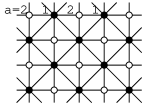
Figure 1: The square-diagonal (Union Jack) lattice. The decomposition of $V$ consists of two classes: $V_{1}=\{\bullet\}$ and $V_{2}=\{\circ\}$.

The decomposition of $V$ consists of two classes $V_{1}=\{\bullet\}$ and $V_{2}=\{\circ\}$. The matrix $q_{ab}$ is given by

$$q=\begin{pmatrix}4&4\\ 4&0\\ \end{pmatrix}.$$ (18)

Each class has an equal number of vertices: $N_{1}=N_{2}=\frac{1}{2}N.$ I assume that the sublattice structure is respected at the boundary.

The field configuration $x_{1}=8/\delta,x_{2}=\delta$ becomes a saddle point in the limit $\delta\rightarrow 0$. Eq. (17) yields

$$\omega_{\mathrm{SP}}^{\mathrm{SD}}=\frac{4}{e}$$ (19)

which is, surprisingly, exactly the same value as the simple square lattice. It means that the $\mathcal{H}(G)$ of the square-diagonal lattice grows no faster than that of the simple square lattice though the former has many additional diagonal edges. It turns out that it is the case; the simple square lattice and the corresponding square-diagonal lattice have exactly the same number of Hamiltonian cycles, which I prove rigorously in subsection 5.1.

4.2 Square-triangular type lattices

As another example of the use of (17), I apply it to a series of inhomogeneous square-triangular lattices $D(t,u)$ and $V(t,u)$ depicted in Fig. 2.

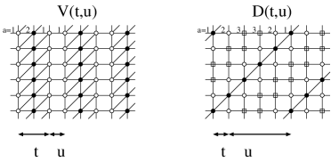
Figure 2: Square-triangular lattices $V(t=2,u=1)$ and $D(t=1,u=4)$. The integers $t$ and $u$ are the numbers of plaquettes with and without diagonal edges, respectively, consecutive in the horizontal direction. The sublattices are distinguished by the shape of the vertices.

They are square lattices with some of the diagonal edges added. The matrices $q$ for them are all tridiagonal matrices if one labels sublattices appropriately. Here I show the $m\times m$ matrix $q$ and the fraction $N_{a}/N$ of $V(t=1,u=2m-1)$ and $D(t=1,u=2m-3)$, $m=(1),2,3,\ldots$.

Lattice $V(1,2m-1)$

$$q=\left(\begin{smallmatrix}4&1&0&0&\cdots&0\\ 1&2&1&0&&\vdots\\ 0&1&2&\ddots&\ddots&\vdots\\ 0&0&\ddots&\ddots&1&0\\ \vdots&&\ddots&\ddots&2&1\\ &&&&&\\ 0&\cdots&\cdots&0&1&3\\ \end{smallmatrix}\right),\quad\frac{N_{a}}{N}=\frac{1}{m}\quad(a=1,\ldots,m).$$ (20)

Lattice $V(1,2m-2)$

$$q=\left(\begin{smallmatrix}4&1&0&0&\cdots&0\\ 1&2&1&0&&\vdots\\ 0&1&2&\ddots&\ddots&\vdots\\ 0&0&\ddots&\ddots&1&0\\ \vdots&&\ddots&\ddots&2&2\\ &&&&&\\ 0&\cdots&\cdots&0&1&2\\ \end{smallmatrix}\right),\quad\frac{N_{a}}{N}=\begin{cases}\frac{1}{2m-1}&(a=m),\\ \frac{2}{2m-1}&(\text{otherwise}).\end{cases}$$ (21)

Lattice $V(2m-1,1)$

$$q=\left(\begin{smallmatrix}3&2&0&0&\cdots&0\\ 2&2&2&0&&\vdots\\ 0&2&2&\ddots&\ddots&\vdots\\ 0&0&\ddots&\ddots&2&0\\ \vdots&&\ddots&\ddots&2&4\\ &&&&&\\ 0&\cdots&\cdots&0&2&2\\ \end{smallmatrix}\right),\quad\frac{N_{a}}{N}=\frac{1}{m}\quad(m=1,\ldots,m).$$ (22)

Lattice $V(2m-2,1)$

$$q=\left(\begin{smallmatrix}3&2&0&0&\cdots&0\\ 2&2&2&0&&\vdots\\ 0&2&2&\ddots&\ddots&\vdots\\ 0&0&\ddots&\ddots&2&0\\ \vdots&&\ddots&\ddots&2&2\\ &&&&&\\ 0&\cdots&\cdots&0&2&4\\ \end{smallmatrix}\right),\quad\frac{N_{a}}{N}=\begin{cases}\frac{1}{2m-1}&(a=m),\\ \frac{2}{2m-1}&(\text{otherwise}).\end{cases}$$ (23)

Lattice $D(1,2m-3)$

$$q=\left(\begin{smallmatrix}2&2&0&0&\cdots&0\\ 4&0&2&0&&\vdots\\ 0&2&0&\ddots&\ddots&\vdots\\ 0&0&\ddots&\ddots&2&0\\ \vdots&&\ddots&\ddots&0&4\\ &&&&&\\ 0&\cdots&\cdots&0&2&0\\ \end{smallmatrix}\right),\quad\frac{N_{a}}{N}=\begin{cases}\frac{1}{2m-2}&(a=1,m),\\ \frac{2}{2m-2}&(\text{otherwise}).\end{cases}$$ (24)

Lattice $D(1,2m-2)$

$$q=\left(\begin{smallmatrix}2&2&0&0&\cdots&0\\ 4&0&2&0&&\vdots\\ 0&2&0&\ddots&\ddots&\vdots\\ 0&0&\ddots&\ddots&\ddots&0\\ \vdots&&\ddots&\ddots&0&2\\ &&&&&\\ 0&\cdots&\cdots&0&2&2\\ \end{smallmatrix}\right),\quad\frac{N_{a}}{N}=\begin{cases}\frac{1}{2m-1}&(a=1),\\ \frac{2}{2m-1}&(\text{otherwise}).\\ \end{cases}$$ (25)

Lattice $D(2m-3,1)$

$$q=\left(\begin{smallmatrix}0&2&0&0&\cdots&0\\ 4&2&2&0&&\vdots\\ 0&2&2&\ddots&\ddots&\vdots\\ 0&0&\ddots&\ddots&2&0\\ \vdots&&\ddots&\ddots&2&4\\ &&&&&\\ 0&\cdots&\cdots&0&2&2\\ \end{smallmatrix}\right),\quad\frac{N_{a}}{N}=\begin{cases}\frac{1}{2m-2}&(a=1,m),\\ \frac{2}{2m-2}&(\text{otherwise}).\\ \end{cases}$$ (26)

Lattice $D(2m-2,1)$

$$q=\left(\begin{smallmatrix}0&2&0&0&\cdots&0\\ 4&2&2&0&&\vdots\\ 0&2&2&\ddots&\ddots&\vdots\\ 0&0&\ddots&\ddots&2&0\\ \vdots&&\ddots&\ddots&2&2\\ &&&&&\\ 0&\cdots&\cdots&0&2&4\\ \end{smallmatrix}\right),\quad\frac{N_{a}}{N}=\begin{cases}\frac{1}{2m-1}&(a=1),\\ \frac{2}{2m-1}&(\text{otherwise}).\\ \end{cases}$$ (27)

For small $m$, eq. (15) can be solved analytically. For example, $V(1,3)$ turns out to possess the saddle point

$$\frac{x_{1}}{2}=\frac{x_{2}}{3}=\sqrt{2+\frac{1}{\sqrt{3}}},$$ (28)

which implies

$$\omega_{\mathrm{SP}}^{V(1,3)}=\frac{1+2\sqrt{3}}{e}=1.64225\cdots.$$ (29)

As $m$ increases, one is forced to solve eq. (15) numerically. Fig. 3 illustrates the dependence of $\log\omega_{\mathrm{SP}}$ of $V(t,u)$ ($\diamond$) and $D(t,u)$ ($\circ$) on $f:=t/(t+u).$

Figure 3: The estimates for $\omega$ are plotted. The saddle point approximation $\omega_{\mathrm{SP}}$ for $V(t,u)$ ($\diamond$) and $D(t,u)$ ($\circ$) with $2t+u\lesssim 16$ are compared with the result of transfer matrix calculation $\omega_{\mathrm{TM}}$ ( $\square$ and $\times$ with an error bar, respectively). For details at $f=1/2,1/3$, see Table 1.

Note that $f=0,1$ correspond to the simple square lattice and the triangular lattice, respectively.

For the purpose of comparison, I also plot an estimate $\omega_{\mathrm{TM}}$, the result of numerical diagonalization of the transfer matrices for $V(t,u)$ ($\square$) and $D(t,u)$ ($\times$). The method to calculate $\omega_{\mathrm{TM}}$ is explained later in section 6. Here I only mention that, under plausible assumptions, $\omega_{\mathrm{TM}}$ agrees with the true value $\omega$ within the precision of the numerical work and the error originating from the finite size effects, though it takes considerable memory and CPU time to compute it. On the other hand, calculating $\omega_{\mathrm{SP}}$ is quite easy.

I argue that the estimates $\omega_{\mathrm{SP}}$ capture the qualitative feature of $\omega_{\mathrm{TM}}$ though there is a certain amount of difference in the numerical values.

First of all, one notices that $\omega_{\mathrm{SP}}$ for $D(1,2m-3)$ is saturated just like the square-diagonal lattice:

$$\omega_{\mathrm{SP}}^{D(1,2m-3)}=\frac{4}{e}\quad(m=2,3,\ldots).$$ (30)

This suggests that the diagonal edges contribute almost nothing to $\mathcal{H}(D(1,2m-3))$.

In accordance with this fact, the numerical estimate $\omega_{\mathrm{TM}}^{D(1,2m-3)}$ also stays identical with $\omega_{\mathrm{TM}}$ of the simple square lattice. I will argue in subsection 5.2 that $\omega$ for $D(1,2m-3)$ and that for the simple square lattice should in fact be identical.

In the field theory, the saddle point for $D(1,2m-3)$ is given by

$$x_{2a+1}=8/\delta,\quad x_{2a}=\delta\quad(\delta\rightarrow 0).$$ (31)

It is intriguing that one needs the limiting procedure $\delta\rightarrow 0$ whenever one obtains the saturated value $\omega_{\mathrm{SP}}=4/e$.

Secondly, apart from the series $D(1,2m-3)$, the estimate $\omega_{\mathrm{SP}}$ increases with $f$ for both $V(t,u)$ and $D(t,u)$ as naturally expected. The result for $\omega_{\mathrm{TM}}$ confirms this naive expectation. Moreover, in both analysis, $\omega_{\mathrm{SP/TM}}$ for $D(t,u)$ is always slightly lower than $V(t,u)$ for a fixed $(t,u)$.

Lastly, some detailed structures of $\omega_{\mathrm{TM}}$ are reproduced in $\omega_{\mathrm{SP}}$. For example, there is a violation of simply-increasingness of $\omega_{\mathrm{TM}}$ for the pair $D(2,1)$ and $D(3,2)$. It is present also for $\omega_{\mathrm{SP}}$.

Near $f=1$, there is a considerable difference between the numerical values of $\omega_{\mathrm{SP}}$ and $\omega_{\mathrm{TM}}$. Note, however, this difference is already there for the triangular lattice, for which the mean field saddle point approximation (3) has been applied. Thus, this difference does not imply the fault of the extension (17).

5 Exact relations among $\mathcal{H}(G)$

I prove some equalities among $\mathcal{H}(G)$ for the square-diagonal lattice and the square-triangular type lattices.

5.1 Square-diagonal lattice

Let $G_{\mathrm{SD}}$ be a square-diagonal lattice of a rectangular shape with $L_{x}\times L_{y}=N$ vertices. The periodic boundary condition is imposed across the edges of the rectangle giving $G_{\mathrm{SD}}$ the toric topology. I assume that $L_{x}$ and $L_{y}$ are even and the square-diagonal lattice structure is consistent with the boundary condition. I define a simple square lattice $G_{\mathrm{SS}}$ as the lattice obtained by removing all the diagonal edges from $G_{\mathrm{SD}}$. It also has $N$ vertices. I shall prove $\mathcal{H}(G_{\mathrm{SD}})=\mathcal{H}(G_{\mathrm{SS}})$. In other words, I will show that Hamiltonian cycles on $G_{\mathrm{SD}}$ passes vertical and horizontal edges but not diagonal edges.

I decompose the set of vertices of $G_{\mathrm{SD}}$ into $V_{1}$ and $V_{2}$ as depicted in Fig. 1. Then $N_{1}=N_{2}=N/2$. On a Hamiltonian cycle, there are $N$ vertices and $N$ edges. Suppose $N^{(d)}$ edges out of $N$ are diagonal ones. The two ends of a diagonal edge belong to $V_{1}$. On the other hand, there are $N-N^{(d)}$ vertical or horizontal edges each of which connects $V_{1}$ and $V_{2}$. Thus I have

$$N_{1}=\left(2\times N^{(d)}+1\times(N-N^{(d)})\right)\times\frac{1}{2}$$ (32)

and

$$N_{2}=(N-N^{(d)})\times\frac{1}{2}$$ (33)

which imply $N^{(d)}=0$.

Because $\mathcal{H}(G_{\mathrm{SD}})=\mathcal{H}(G_{\mathrm{SS}})$ for $G_{\mathrm{SD}}$ and $G_{\mathrm{SS}}$ at any finite size, one can take the limit $N\rightarrow\infty$ to have $\omega^{\mathrm{SD}}=\omega^{\mathrm{SS}}$.

5.2 Lattice $D(1,2m-3)$

Let $G_{m}$ be a finite $D(1,2m-3)$ lattice of a rectangular shape. Again I assume the periodic boundary condition on both directions, respecting the $D(1,2m-3)$ structure at the boundary. I shall show $\mathcal{H}(G_{m})=\mathcal{H}(G_{\mathrm{SS}})$.

For brevity, I write $G\sqsubset G^{\prime}$ if $V=V^{\prime}$ and $E\subset E^{\prime}$, where $G=(V,E)$ and $G^{\prime}=(V^{\prime},E^{\prime})$. Apparently, $\mathcal{H}(G)\leq\mathcal{H}(G^{\prime})$ if $G\sqsubset G^{\prime}$. We have seen that the inequality $\mathcal{H}(G_{\mathrm{SS}})\leq\mathcal{H}(G_{\mathrm{SD}})$ for the pair $G_{\mathrm{SS}}\sqsubset G_{\mathrm{SD}}$ is actually an equality.

It is crucial to find that $G_{\mathrm{SS}}\sqsubset G_{m}\sqsubset G_{\mathrm{SD}}$. Thus, I obtain $\mathcal{H}(G_{\mathrm{SS}})=\mathcal{H}(G_{m})$. This relation, in the limit $N\rightarrow\infty$, again implies that $\omega^{\mathrm{SS}}=\omega^{D(1,2m-3)}$.

6 Numerical transfer matrix method

In order to estimate $\omega$ numerically, I map the problem of Hamiltonian cycles onto the zero fugacity limit of the fully packed loop model. Then I represent the fully packed model onto a state sum model with a local weight in order to construct a row transfer matrix. The quantity $\omega$ is related to an eigenvalue of the transfer matrix.

The partition function of the fully packed model with the the loop fugacity $n$ is given by

$$Z_{\mathrm{FPL}}(n)=\sum_{\text{fully packed loop configuration}}n^{\mathcal{N}_{\mathrm{L}}}.$$ (34)

The sum in (34) is over all the fully packed loop configurations (Fig. 4), that is non-intersecting closed loops on the lattice such that every vertex is visited by exactly one of the loops. The number of connected components of loops, denoted by $\mathcal{N}_{\mathrm{L}}$, can be greater than one.

Figure 4: An example of fully packed loop configuration with $\mathcal{N}_{\mathrm{L}}=8$ on the simple square lattice $V(0,1)$ . The loops are drawn in thick lines.

One can construct an equivalent state sum model in the following way. One begins with the triangular lattice $V(1,0)$ with the coordination number $q=6$. The local degrees of freedom $z$ live on each edge $e$. The three possible values of $z(e)$ is $\leftarrow$ (a directed edge), $\rightarrow$ (an oppositely directed edge ), and $-$ (a vacant edge). Let $e_{1},\ldots,e_{6}$ be the edges that share a vertex $r$. States on $e_{1},\ldots,e_{6}$ interact on $r$. The local vertex weight is

$$W(z(e_{1}),\ldots,z(e_{6}))=s^{k}\quad(s\in\mathbb{C})$$ (35)

if there is exactly one ingoing arrow and an outgoing one at $r$, where the integer $k$ is given by

$$k=\frac{(\text{the angle of the right turn})}{\pi/4}.$$ (36)

as illustrated in Fig. 5.

Figure 5: A vertex weight for the state sum model for the fully packed loop model. The parameter $s$ is a complex number. Other configurations are prohibited ( weight $W=0$ ).

Otherwise, $W=0$.

In other lattices $D(t,u)$ and $V(t,u)$, some of the diagonal edges in the lattice $V(1,0)$ are missing. One extends the above construction to them by just interpreting these missing edges as existing edges on which only the vacant edge state is allowed.

The partition function of the state sum model is given by

$$Z(s):=\sum_{z(e)=\leftarrow,-,\rightarrow\quad(e\in E)}\quad\quad\prod_{r\in V}W(z(e_{j_{1}}),\ldots,z(e_{j_{6}})).$$ (37)

Edges $e_{j_{1}},\ldots,e_{j_{6}}$ are understood to share a vertex $r$. One sees that the surviving configurations in the state sum model are nothing but the fully packed loop configurations with a direction associated with each loop component. Let us inspect a contribution from a loop. When one walks along the loop in the associated direction to come back to the original point, one has changed the direction $\pm 2\pi$ in total (if it is a topologically trivial loop). Therefore, the product of the vertex weight on the loop is $s^{\pm 8}$ due to the choice (36). This is why the partition function of the state sum model agrees with (34) with

$$n=s^{8}+s^{-8}.$$ (38)

Now one can think of a row transfer matrix $\mathbf{T}$ of the fully packed loop model. For the lattices $D(t,u)$ and $V(t,u)$, one introduces a transfer matrix which maps a state on a row of vertical and horizontal edges onto that on the upper row in Fig. 2. That is, a state acted by $\mathbf{T}$ is a linear combination of an arrow configuration on the row $|/|/|/|/\cdots/|/|$. For the lattice $D(t,u)$, a one-unit shift in the horizontal direction is included in $\mathbf{T}$ to take care of the change of the positions of diagonal edges.

It is important to note that the transfer matrix $\mathbf{T}$ commutes with the operator giving the net number of upward arrows

$$d=(\#\uparrow)+(\#\nearrow)-(\#\downarrow)-(\#\swarrow).$$ (39)

Thus $\mathbf{T}$ is block-diagonalized as $\mathbf{T}=\oplus_{d}\mathbf{T}_{d}$.

One considers an infinite cylinder geometry which is suitable for numerical transfer matrix calculation. The horizontal direction is compactified with the period $L$ as indicated in Fig. 6. In the $d=0$ sector there can be loops which wind the cylinder once. It gives rise to a complication because such a loop contributes $s^{0}+s^{0}=2$, not $s^{8}+s^{-8}=n$. To avoid this, one introduces a seam as in Fig. 6. One declares that a loop which goes across the seam from the left to the right should gain an additional weight $s^{8}$, while the left-going one should gain $s^{-8}$.

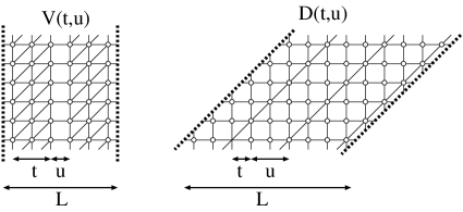
Figure 6: Square-triangular lattices $V(t=2,u=1)$ and $D(t=1,u=2)$. The periodic boundary condition in the horizontal direction is introduced to give the lattice infinite cylinder topology. The seam is indicated by broken lines.

Hamiltonian cycles are encoded in the $d=0$ sector in the limit $n\rightarrow 0$, or $s\rightarrow\exp[\pm\tfrac{\pi i}{16}]$ on the infinite cylinder. The condition $d=0$ excludes the configurations which have unbalanced strings which travels from an end to the other end of the cylinder. The limit $n\rightarrow 0$ excludes small disconnected loops. In the following, $n$ is simply set to zero. The connectivity constant $\omega_{\mathrm{TM}}(L)$ for this geometry is given by

$$\log\omega_{\mathrm{TM}}(L)=\frac{1}{L}\log|\lambda_{0}^{0}(L)|,$$ (40)

where $\lambda^{i}_{d}(L)$ is the $i$-th largest (in the absolute value) eigenvalue of $\mathbf{T}_{d}(L)$. One expects that, by taking the $L\rightarrow\infty$ limit, one arrives at the bulk value $\omega_{\mathrm{TM}}=\omega_{\mathrm{TM}}(\infty)$. The values of $\omega_{\mathrm{TM}}$ in Fig. 3 have been calculated in this way.

I notice that that the relation $\omega_{\mathrm{TM}}^{\mathrm{SS}}=\omega_{\mathrm{TM}}^{\mathrm{SD}}=\omega_{\mathrm{TM}}^{D(1,2m-3)}$ holds already at every finite $L$.

I assume that the rotational symmetry is restored in the $L\rightarrow\infty$ limit with the sound velocity $v=1$ and that the system is described by a conformal field theory [18], which is the case for the simple square lattice $V(0,1)$. For other lattice, one observes, at least, the mass gap closes at $L\rightarrow\infty$. Then scaling exponents are related to the finite size behavior of other eigenvalues of the transfer matrix [19, 20]. The central charge $c$ appears as

$$\log\omega_{\mathrm{TM}}(L)=\frac{1}{L}\log|\lambda^{0}_{0}(L)|=\log\omega_{\mathrm{TM}}(\infty)+\frac{\pi c}{6L^{2}}+\mathcal{O}(L^{-4}).$$ (41)

The correlation lengths $\xi_{i}$ and the scaling dimensions $X_{i}$ of general geometric operators labeled by $i$ are given by [14]

$$\xi_{i}^{-1}=\log\frac{|\lambda^{0}_{i}(L)|}{|\lambda^{0}_{0}(L)|}=\frac{2\pi X_{i}}{L}+\mathcal{O}(L^{-3}).$$ (42)

In particular, the geometric scaling exponents $X_{1}$ and $X_{2}$ (corresponding to one and two spanning strings, respectively) are related to the conformational exponent $\gamma$ in eq. (1) by

$$\gamma=2(1-X_{1})\nu,\quad\frac{1}{\nu}=2-X_{2}.$$ (43)

The result of the finite size scaling analysis is shown in Table 1.

lattice	$L_{\text{max}}$	$c$	$X_{1}$	$\log\omega_{\mathrm{TM}}$	$\log\omega_{\mathrm{SP}}$
$V(0,1)_{L\equiv 0\bmod 2}$	14	$-1.000(11)$	$-0.04423(81)$	0.387171(1)	0.386294
$V(0,1)_{L\equiv 1\bmod 2}$	13	$-2.510(5)$	$-0.1875(10)$	0.387168(2)	0.386294
$V(1,0)_{L\equiv 0\bmod 3}$	9	$-2.06(8)$	$-0.196(18)$	0.74088(7)	0.791761
$V(1,1)$	12	$-1.98(9)$	$-0.175(17)$	0.563057(18)	0.609438
$V(1,2)$	12	$-2.00(4)$	$-0.189(3)$	0.498809(3)	0.532186
$D(1,2)$	12	$-1.98(10)$	$-0.186(25)$	0.470379(3)	0.495166
$V(2,1)$	9	$-1.93(9)$	$-0.183(19)$	0.619823(4)	0.665920
$D(2,1)$	9	$-1.98(3)$	$-0.189(14)$	0.571025(1)	0.617343
$V(1,3)$	12	$-1.90(29)$	$-0.176(3)$	0.46905(4)	0.496068
$V(2,2)$	12	$-1.89(18)$	$-0.216(10)$	0.55761(4)	0.612848
$D(2,2)$	12	$-1.90(14)$	$-0.203(10)$	0.53917(3)	0.574521
$V(3,1)$	8	$-1.87(18)$	$-0.174(10)$	0.650(15)	0.698199
$D(3,1)$	8	$-2.01(18)$	$-0.187(10)$	0.609(16)	0.653694
$V(1,4)$	10	$-2.09(11)$	$-0.187(4)$	0.452(11)	0.474064
$D(1,4)$	10	$-2.10(11)$	$-0.177(4)$	0.427(11)	0.442671
$V(2,3)$	10	$-1.94(11)$	$-0.170(3)$	0.522(10)	0.553356
$D(2,3)$	10	$-2.08(11)$	$-0.189(3)$	0.492(11)	0.524924
$V(3,2)$	10	$-2.02(11)$	$-0.189(3)$	0.595(11)	0.634758
$D(3,2)$	10	$-1.99(11)$	$-0.185(3)$	0.579(10)	0.616846
$V(4,1)$	10	$-1.95(11)$	$-0.184(3)$	0.668(10)	0.716732
$D(4,1)$	10	$-1.92(11)$	$-0.180(3)$	0.636(10)	0.683031
$V(1,5)$	12	$-2.24(8)$	$-0.213(3)$	0.441(8)	0.459443
$V(2,4)$	12	$-2.19(8)$	$-0.210(3)$	0.499(8)	0.525490
$D(2,4)$	12	$-2.07(8)$	$-0.192(3)$	0.482(7)	0.508479
$V(3,3)$	12	$-2.04(8)$	—	0.559(8)	0.593499
$D(3,3)$	12	-2.00(8)	—	0.530(8)	0.564561
$V(1,6)$	14	$-2.02(6)$	—	0.432(5)	0.459443
$D(1,6)$	14	$-2.10(6)$	—	0.411(6)	0.386294

Table 1: Exponents and the entropy per vertex estimated by the numerical transfer matrix method. Lattices $D(1,2m-3)$ are suppressed because they share the properties with $V(0,1)$. The integer $L_{\mathrm{max}}$ is the largest $L$, the size of the lattice in the horizontal direction, which has been examined. The exponent $X_{2}$ is also measured and is found to be zero for all the lattices.

I have treated even and odd $L$ separately for $V(0,1)$ because there is an oscillatory behavior of period 2 due to the twist-like operator insertion [13]. I also see a period-3 oscillation for $V(1,0)$. Presence of such oscillations is not assumed for analysis of other lattices. I find that the exponent $X_{2}$ is always zero at finite $L$ and is supposed to be so in the limit $L\rightarrow\infty$.

The result in Table 1 suggests that, except for $V(0,1)(=D(0,1))$ and $D(1,2m-3)$, the system lies in the same universality class as the dense phase of O($n$) loop model at $n=0$ whose exponents are

$$\begin{split}c=-2,\quad X_{1}=-\frac{3}{16}=-0.1875,\quad X_{2}=0,\\ \nu=\frac{1}{2},\quad\gamma=\frac{19}{16}=1.1875.\end{split}$$ (44)

This fact can be understood well by regarding the fully packed loop model as a special case of the O($n$) loop model whose partition function is given by

$$Z_{\mathrm{loop}}(n,x^{-1})=\sum_{\text{loop configuration}}x^{\mathcal{N}_{\mathrm{V}}-N}n^{\mathcal{N}_{\mathrm{L}}},$$ (45)

where the summation is over all the non-intersecting loop configurations not necessarily fully packed. Thus, the number $\mathcal{N}_{\mathrm{V}}$ of vertices visited by a loop can be different from $N$. In the two parameter space $(n,x^{-1})$, the dense phase emerges in the region where the O($n$) temperature $|x^{-1}|$ is small enough while the fully packed loop model is reproduced by setting $x^{-1}$ to exactly zero.

For the simple square lattice and the hexagonal lattice, the line $x^{-1}=0$ is an unstable critical line where a new universality emerges. This is due to the symmetry $x^{-1}\leftrightarrow-x^{-1}$. Actually, this symmetry holds because any loops on the simple square lattice visit even number of vertices.

The result in Table 1 means that $x^{-1}=0$ is not special for other lattices. This is because they admit loops which visit odd number of vertices [13].

7 Summary

I have estimated the number Hamiltonian cycles on inhomogeneous graphs analytically and numerically. To estimate it analytically, I have employed the field theoretic representation and have applied the saddle point method. A formula for $\omega$ for graphs with sublattice structures has been obtained. The numerical estimation is based on the diagonalized the transfer matrix of the fully packed model on the infinite cylinder geometry.

The former result is simple and is believed to capture the physics of Hamiltonian cycles. The latter is accurate and provides with the scaling exponents though it spends lots of computer time. The results agree each other qualitatively. It is confirmed that the success of the estimate $\omega_{\mathrm{SP}}=3/e,4/e$ and $6/e$ by the former method was not accidental; it now works fine for a family of lattices yielding various values of $\omega_{\mathrm{SP}}$. Moreover, the former method successfully predicts the relation $\omega^{\mathrm{SS}}=\omega^{\mathrm{SD}}=\omega^{D(1,2m-3)}$.

The relation $\omega_{\mathrm{SP}}^{G}\leq\omega_{\mathrm{SP}}^{G^{\prime}}$ holds for all the pairs $G\sqsubset G^{\prime}$ I have examined so far. It may be proved that this holds generally.

The latter method is useful in calculating the exact value of $\mathcal{H}(G)$ of $G$ with the planar or cylinder topology. There seems to be, however, no simple way to apply this method to the lattices with the torus and the higher-genus topology, and three-dimensional lattices. This is due to the presence of numerous topological sectors of self-avoiding loops on the lattice [21]. In contrast, the field theoretic approach was able to predict a boundary condition dependence of $\mathcal{H}(G)$ for a family of toric lattices [12]. Therefore two approaches are considered complementary each other.

References

- [1] J. des Cloizeaux and G. Jannik, Polymers in solution: their modelling and structure, Clarendon Press, Oxford, 1987.
- [2] J. Bascle, T. Garel, and H. Orland, Mean-field theory of polymer melting, J. Phys. A 25 (1992) L1323.
- [3] H. S. Chan and K. A. Dill, Compact polymers, Macromolecules 22 (1989) 4559.
- [4] C. J. Camacho and D. Thirumalai, Minimum energy compact structures of random sequences of heteropolymers, Phys. Rev. Lett. 71 (1993) 2505.
- [5] S. Doniach, T. Garel, and H. Orland, Phase diagram of a semiflexible polymer chain in a solvent: application to protein folding problem, J. Chem. Phys. 105 (1996) 1601.
- [6] T. G. Schmalz, G. E. Hite, and D. J. Klein, Compact self-avoiding circuits on two-dimensional lattices, J. Phys. A 17 (1984) 445.
- [7] A. L. Owczarek, T. Prellberg, and B. R., New scaling Form for the collapsed polymer phase, Phys. Rev. Lett. 70 (1993) 951.
- [8] A. Malakis, Hamiltonian walks and polymer configutions, Physica 84A (1976) 256.
- [9] B. Duplantier and F. David, Exact partition functions and correlations functions of multiple Hamiltonian walks on the Manhattan lattice, J. Statist. Phys. 51 (1988) 327.
- [10] H. Orland, C. Itzykson, and C. de Dominicis, An evaluation of the number of Hamiltonian paths, J. Physique 46 (1985) L353.
- [11] J. Suzuki, Evaluation of the connectivity of Hamiltonian paths on regular lattices, J. Phys. Soc. Japan 57 (1988) 687.
- [12] S. Higuchi, Field theoretic approach to the counting problem of Hamiltonian cycles of graphs, Phys. Rev. E58 (1998) 128, cond-mat/9711152.
- [13] M. T. Batchelor, H. W. J. Blöte, B. Nienhuis, and C. M. Yung, Critical behaviour of the fully packed loop model on the square lattice, J. Phys. A 29 (1996) L399.
- [14] B. Duplantier and H. Saleur, Exact critical properties of two-dimensional dense self-avoiding walks, Nucl. Phys. B290[FS20] (1987) 291.
- [15] J. L. Jacobsen and J. Kondev, Field theory of compact polymers on the square lattice, Nucl. Phys. B532[FS] (1998) 635, cond-mat/9804048.
- [16] M. Batchelor, J. Suzuki, and C. Yung, Exact results for Hamiltonian walks from the solution of fully packed model on the honeycomb lattice, Phys. Rev. Lett. 73 (1994) 2646, cond-mat/9408083.
- [17] M. R. Garey and D. S. Johnson, Computers and intractability — A guide to the theory of NP-completeness, W. H. Freeman, San Francisco, 1979.
- [18] A. Belavin, A. Polyakov, and A. Zamolodchikov, Infinite conformal symmetry in two dimensional quantum field theory, Nucl. Phys. B241 (1984) 333.
- [19] H. W. J. Blöte, J. L. Cardy, and M. P. Nightingale, Conformal invariance the central charge and universal finite-size amplitudes at criticality, Phys. Rev. Lett. 56 (1986) 742.
- [20] I. Affleck, Universal tem in the free energy at a critical point and the conformal anomaly, Phys. Rev. Lett. 56 (1986) 746.
- [21] S. Higuchi, Hamiltonian cycles on random lattices of arbitrary genus, Nucl. Phys. B540 (1999) 731, cond-mat/9806349.