Optimal packing of polydisperse hard-sphere fluids

Abstract

We consider the effect of intermolecular interactions on the optimal size-distribution of $N$ hard spheres that occupy a fixed total volume. When we minimize the free-energy of this system, within the Percus-Yevick approximation, we find that no solution exists beyond a quite low threshold ( $\eta\thickapprox 0.260$). Monte Carlo simulations reveal that beyond this density, the size-distribution becomes bi-modal. Such distributions cannot be reproduced within the Percus-Yevick approximation. We present a theoretical argument that supports the occurrence of a non-monotonic size-distribution and emphasizing the importance of finite size effects.

I Introduction

Synthetic colloids are never perfectly monodisperse. Often, this polydispersity is a drawback—for instance, polydispersity is a problem in the preparation of high-quality colloidal crystals, that are needed in photonic bandgap materials. However, occasionally, polydispersity is desirable, because it allows us to achieve material properties that cannot be realized with monodisperse colloids. For instance, monodisperse colloidal systems can fill at most 74.05 % of space in the crystalline phase (regular close packing) and some 63% in the liquid/glassy state (random close packing). In contrast, colloids with a properly chosen particle-size distribution can be made essentially space filling, both in the crystalline solid (Appolonian packing) and in the liquid. In practice, perfect space filling structures are never achieved because this requires an infinite number of (predominantly small) particles per unit volume. Here, we consider a somewhat simpler problem, namely the filling of a given volume $V$ by a fixed number of particles $N$, that occupy a prescribed total volume fraction $\eta$. We assume that the particles are free to exchange volume. As we have fixed both the number and the total volume of the particles, the average volume per particle is fixed—it defines the natural length-scale in the model. Clearly, the Helmholtz free energy of the system will depend on the non-fixed particle-size distribution. The distribution, however, is restricted by the two constraints of fixed number of particles and fixed total volume. We define the optimal size distribution to be the one that minimizes the Helmholtz free energy under both constraints. In the Monte Carlo simulations (performed in the isothermal-isobaric ensemble) that we report in this paper, we study the density dependence of the particle-size distribution. We compare the simulation results for the size distribution with an analytical estimate that is obtained by solving the Percus-Yevick (PY) equation for an $N$-component hard-sphere mixture[1]. Not surprisingly, the PY equation works very well at low densities. However, the theory breaks down at a surprisingly low density ($\eta\thickapprox$0.26). Of course, the fact that an approximate theory fails at a given density, does not imply that there is anything special going on in the system at that density. Yet, our simulations indicate that there is—the size distribution that was initially uni-modal, becomes bi-modal. We present a theoretical argument supporting this scenario.

The remainder of this paper is organized as follows: in section II we describe the constant-pressure Monte Carlo simulations. The Percus-Yevick expression for the free energy of a system of polydisperse hard spheres with variable size distribution is discussed in section III and IV. Section V is devoted to the derivation of analytical results turning useful when interpreting the simulation data. The mechanism behind the transition from uni-modal to bi-modal size distribution is also discussed.

II Monte Carlo Simulations

Monte Carlo simulations were performed in the isothermal-isobaric (constant $NPT$) ensemble [6]. This means that the number of particles $N$, the pressure $P$ and the temperature $T$ are fixed. We attempt three distinct types of trial moves. We change the positions of the particles and allow the volume of simulation box to fluctuate, in order to equilibrate with respect to the applied pressure. Since we do not expect any crystalline order at low pressures, a cubic box shape is maintained. The third type of move is the one related to sampling the polydispersity of the system. To this end, we select two particles at random, between which we exchange an amount of volume drawn uniformly from the interval $[-\Delta V_{max},\Delta V_{max}]$ (Fig. 1). The maximum volume change ${\Delta V_{max}}$ was chosen such that the acceptance of a volume exchange move is between 35 and 50 %. The relative frequency of the three moves is given by $N:1:N/2$. The initial configurations are made by $N$ monodisperse spheres on a simple cubic lattice.

Simulations were performed for system sizes of $N$=512 or 1000, and several different reduced pressures ${P}^{*}=(k_{B}T)^{-1}P\langle\sigma^{3}\rangle$, where $\sigma$ is the diameter of particles, and $\langle\cdot\rangle$ denotes an average over particle-size distribution. As $\langle\sigma^{3}\rangle$ is fixed, we choose $\langle\sigma^{3}\rangle^{1/3}$ to define the unit of length that we will use in the remainder of this paper. We use $k_{B}T$ as our unit of energy. All other units that we need, follow from these definitions. The equation of state [${P}^{*}$ as a function of ${\rho}^{*}(\equiv\rho\langle\sigma^{3}\rangle)$] and the particle size distribution function were determined in the simulations. The results for the equation of state are shown in Fig. 2. The simulation data have been collected in Table I. At low pressures the particle-size distribution function is a single-peaked function with its maximum at $v=0$ (Figs. 3, 4 and 5). At higher pressures (typically, $P^{*}>2.0$), the particle-size distribution develops a second peak. Actually, this second peak is quite small (i.e. only a small fraction of all particles becomes “large”). However, these particles contribute appreciably to the total volume fraction (Fig. 6). Depending on the pressure this contribution can get as large as 75%.

The formation of big particles in these MC simulations is a rather slow “dynamical” process. In order to speed up calculations, we did additional simulations, in which we started with a bi-disperse distribution, with one or several big particles containing 99% of the total volume occupied by the spheres, surrounded by a sea of small particles containing the remaining volume. In the 512 particle system, only one or two big particles remain for the lower pressures ($P^{*}=2.5$ and $P^{*}=3.0$). For higher pressures the number of big particles can stabilize at higher values as well. For the 1000 particle system the maximum number of big particles observed at the lower pressures is three. In addition, the size of these big particles is not the same. It is not clear whether this suggests a further possible fractionation or that it is a consequence of the slow equilibration and that one or more of the big particles are still shrinking.

Below, we discuss these simulation results in the context of the relevant theoretical predictions, but first let us stop to make certain considerations on the ideal entropy associated with this system.

III Ideal entropy of a polydisperse system

Strictly speaking, the ideal entropy of a polydisperse system is infinite [1]. In a multicomponent system such an entropy is exactly given by

$$-Nk_{B}\sum_{i}w_{i}\ln(\Lambda_{i}^{3}\rho w_{i})\,,$$ (1)

where $w_{i}$ is the molar fraction of species $i$ and $\Lambda_{i}$ its thermal wavelength. The usual path towards the entropy of a polydisperse system [1] (or for that matter, towards the entropy of continuous signals in Information Theory [3]) is to classify the species into “boxes” according to a certain property which distinguishes them (diameter, volume, molecular weight, etc). If $x$ denotes such a property species $i$ will denote the box having particles with $x$ between $i\Delta x$ and $(i+1)\Delta x$, for a given $\Delta x$ which defines the boxes. If $W(x)$ denotes the probability density of a particle having the value $x$ for that property, then $w_{i}=W(x_{i})\Delta x$ where $x_{i}$ is a typical value of the $i$th box. Then Eq. (1) adopts the form

$$-Nk_{B}\sum_{i}W(x_{i})\Delta x\ln(\Lambda_{i}^{3}\rho W(x_{i})/\Delta x)\,.$$ (2)

The entropy of the polydisperse system is obtained from Eq. (2) taking the limit $\Delta\to 0$, and we can clearly see that, besides obtaining the usual expression [1, 3]

$$S_{\rm poly}=-NK_{B}\int dx\,W(x)\ln[\Lambda(x)^{3}W(x)]\,,$$ (3)

there is also a divergent $-\ln\Delta x$, which is simply taken as a “constant” ignorable term.

But expression (3) is not well defined. Suppose we simply change coordinates to label the species from $x$ to $y$ (say, from the diameter to the volume). Then the probability density in the new variable will be $\widetilde{W}(y)=W(x)\left|\frac{dx}{dy}\right|$. It is straightforward to show that in the new labeling the entropy becomes

$$S_{\rm poly}=-NK_{B}\int dy\,\widetilde{W}(y)\ln[\Lambda(x(y))^{3}\widetilde{W}(y)]+Nk_{B}\int dy\,\widetilde{W}(y)\ln\left|\frac{dy}{dx}\right|\,,$$ (4)

which is different of what we would have obtained had we began with the labeling $y$.

This is a well known fact in Information Theory [3]. In the study of fluid equilibria of quenched polydisperse systems this fact turns out to be irrelevant because the new term simply adds the same constant to both sides of the equilibrium equations [4]. However when studying annealed polydispersity this results tells us that the labeling is crucial and has to be dictated by the physical process underlying the polydispersity. In our case the Monte Carlo movements described in Section II are a large scale description of a hypothetical microscopic system of tiny particles of exactly the same size distributed among $N$ aggregates of a variable number of particles. The constant volume constraint would correspond to the conservation of the number of tiny particles, and the natural labeling of the aggregates would be the number of tiny particles which form it. As this number is proportional to the volume of the aggregate, in the continuum description is the volume, instead of the diameter, what turns out to be the natural labeling.

Notice that we could have described another model in which the tiny particles aggregated into spherical surfaces. In that case it would be the total surface what would be preserved and the natural labeling of aggregates would be their respective surfaces. As we will discuss in the conclusions, the physics of this model would be completely different.

IV Percus-Yevick Theory

The Percus-Yevick equation for an $n$-component hard-sphere mixture can be solved analytically, to yield the following equation of state [1]:

$$\frac{\pi}{6}P^{*}=\frac{\xi_{0}}{1-\xi_{3}}+\frac{3\xi_{1}\xi_{2}}{(1-\xi_{3})^{2}}+\frac{3\xi_{2}^{3}}{(1-\xi_{3})^{3}}.$$ (5)

The $j$-th moment of the particle-size distribution $\xi_{j}$ is defined as

$$\xi_{j}=\frac{\pi}{6}\sum_{i}\rho_{i}\left(\frac{6v_{i}}{\pi}\right)^{j/3},$$ (6)

where $\rho_{i}=N_{i}/V$, the index $i$ is used to denote the different particle species, and $v_{i}$ is the volume of the $i$-th species.

Equation (5) is also valid for a continuous size distribution, in which case the sum in Eq. (6) is replaced by an integral. The corresponding expression for the chemical potential of a species with radius $R$ is[2]

$$\mu^{*}=\ln\left[\rho\Lambda^{3}W(v)\right]-\ln(1-\xi_{3})+\frac{6\xi_{2}R}{(1-\xi_{3})}+\frac{12\xi_{1}R^{2}}{(1-\xi_{3})}+\frac{18\xi_{2}^{2}R^{2}}{(1-\xi_{3})^{2}}+\frac{4\pi}{3}P^{*}R^{3}$$ (7)

where $\Lambda$ is the de-Broglie thermal wavelength, $\sqrt{h^{2}/(2\pi mkT)}$, and $W(v)$ is the probability density to find a particle with a volume around $v=(4\pi/3)R^{3}$. The pressure $P^{*}$ is given by Eq. (5).

In an (NPT) description, the Gibbs free energy of the system fulfilling the constraints, must be at a minimum. The conservation of the number of particles and of the solid volume fraction, imply that $W(v)$ must be of the form:

$$W(v)=\exp\left\{\sum_{i=0}^{3}\alpha_{i}R^{i}\right\},$$ (8)

where

$$\alpha_{1} = -\frac{6\xi_{2}}{1-\xi_{3}},$$ (9)

$$\alpha_{2} = -12(\frac{\xi_{1}}{1-\xi_{3}}+\frac{3\xi_{2}^{2}}{2(1-\xi_{3})^{2}}).$$ (10)

The coefficients $\alpha_{0}$ and $\alpha_{3}$ are determined by the constraints that the number of particles and the solid volume fraction are fixed. Note that all  $\xi_{i}$ $(i=1,2,3)$ are positive. Moreover, $\xi_{3}$ is equal to the volume fraction $\eta$, and is therefore necessarily less than one. Hence, $\alpha_{1}$ and $\alpha_{2}$ are always negative. The last coefficient, $\alpha_{3}$, should be negative or zero, because otherwise the particle-size distribution cannot be normalized. Since $\alpha_{1}$, $\alpha_{2}$ and $\alpha_{3}$ are always negative the Percus-Yevick equation predicts that $W(v)$ is a monotonically decreasing function of $v$. This implies that the size-distribution given by Eq. (8) can never be bi-modal.

Note that these conclusions also hold for the more accurate equation of state of Mansoori et al. [5]. This equation adds an extra term to the pressure given in Eq. (5) depending on $\xi_{3}$. Thus Eq. (7) is the same with the new expression for $P$—which turns out to be irrelevant because the $R^{3}$ term is controlled by the Lagrange multiplier associated with the constraint on the total solid particle volume. In other respect, the analysis for the Mansoori equation-of-state is identical to that for PY.

In practice, we solve Eq. (8) numerically. To this end, we represent $W(v)$ as a histogram. Initially, the value of $W(v)$ in the different bins is assigned an arbitrary non-negative value, compatible with the constraint that $W(v)$ is normalized and that $\langle v\rangle$ is fixed. We fix the density at the desired value. We determine the optimal $W(v)$ using the following scheme: we select a bin (say $i$) at random and change the value of $W(v_{i})$ by a random amount $\Delta W$, distributed uniformly in the interval $[-\Delta W_{max},\Delta W_{max}]$. We first check if the new value $W(v_{i})$ is non-negative. If it is, we satisfy the constraints by scaling the width of all bins and the height of the function by two appropriately chosen factors. We then compute all moments $\xi_{j}$, the pressure and the free energy, and we check if the Helmholtz free energy is smaller than the previous one. If it is, we accept the new value for $W(v_{i})$, otherwise we reject it. We repeat the procedure until the free energy no longer decreases. We have verified that $W(v)$ is indeed of the form given by Eqs. (8) through (10). Figure 4 shows a comparison of the PY estimate for $W(v)$, determined in this way, with the results of the full Monte Carlo simulations. We find that $\alpha_{3}$ is a monotonically increasing function of density. A comparison between simulation and PY theory for the equation of state is shown in Fig. 2. Note that, in this figure, the PY solution terminates at pressure $P_{c}\thickapprox 1.34$ (the cross in Fig. 2). This is the point where $\alpha_{3}$ becomes zero. Beyond this point we can no longer find a solution for $W(v)$ that is of the form given by Eq. (8). In Appendix A, we consider the breakdown of the PY theory in more detail and obtain the packing fraction beyond which the PY approximation breaks down: $\eta_{c}=0.260$, the corresponding pressure being $P^{*}_{c}=1.343$. This breakdown of the PY equation at a relatively low density is surprising, as the PY equation works well up to quite high densities for fixed particle size distributions [7, 8, 9]. That it breaks down regardless the accuracy of the equation of state can be inferred from the fact that Mansoori et al.’s equation of state undergoes exactly the same breakdown, though for slightly different values of $\eta$ and $P$. Besides, from the analysis that we have carried out, it can be seen that a similar breakdown will appear for any other theory yielding an equation of state depending only on $\xi_{i}$, $i=0,1,2,3$.

V Analytical results

In this section, we derive a theoretical bound for the pressure of the polydisperse system, providing the equation of state at the packing fraction where the size distribution becomes bi-modal. To this end, we work in the ($NVT$) ensemble and take advantage of the extremality of the Helmholtz free energy under the constraints of constant $N$ and $\eta$: the “grand potential”

$${\cal R}={\cal F}\{W\}-{\cal L}_{0}\int W(v)\,dv-{\cal L}_{1}\int vW(v)\,dv,$$ (11)

where ${\cal L}_{0}$ and ${\cal L}_{1}$ are Lagrange multipliers, has to be minimum for the optimal size distribution. In the above relation, the free energy functional ${\cal F}$ can be cast into the usual ideal and excess contributions

$${\cal F}\{W\}=Nk_{B}T\,\int dv\,W(v)\left[\ln\left(\Lambda^{3}\rho W(v)\right)-1\right]+{\cal F}_{\hbox{excess}}\{W\}.$$ (12)

We attempt the following change in the system: the volume of a given particle $v_{0}$ is increased by an amount $\delta v_{0}$, before a rescaling of all volumes by a factor $\lambda$ (e.g. $v\to\lambda v$) such that the overall volume change vanishes. This imposes:

$$\lambda=1-\frac{\delta v_{0}}{N\langle v\rangle}+{\cal O}\left([\delta v_{0}]^{2}\right).$$ (13)

The effect of the expansion of particle $v_{0}$ on the size-distribution can be written:

$$\delta W(v)=\frac{1}{N}\,\,\left[\,\delta\left(v-v_{0}-\delta v_{0}\right)\,-\,\delta\left(v-v_{0}\right)\,\right],$$ (14)

where $\delta(...)$ denotes the Dirac distribution. The scaling procedure affects $W$ according to

$$\delta W(v) = \frac{1}{\lambda}\,W\!\left(\frac{v}{\lambda}\right)-W(v)$$ (15)

$$= \frac{\delta v_{0}}{N\langle v\rangle}\,\,\frac{d[vW]}{dv}\,+\,{\cal O}\left([\delta v_{0}]^{2}\right).$$ (16)

The corresponding variation of the ideal contribution to ${\cal F}$ reads

$$\delta{\cal F}_{\hbox{id}}=\int dv\,\,\frac{\delta{\cal F}_{\hbox{id}}\{W\}}{\delta W(v)}\,\,\delta W(v),$$ (17)

with the functional derivative

$$\frac{\delta{\cal F}_{\hbox{id}}\{W\}}{\delta W(v)}=Nk_{B}T\,\ln[\Lambda^{3}W(v)].$$ (18)

We then get the entropic term

$$\delta{\cal F}_{\hbox{id}} = k_{B}T\int dv\,\ln[\Lambda^{3}W]\left[\delta\left(v-v_{0}-\delta v_{0}\right)-\delta\left(v-v_{0}\right)+\frac{\delta v_{0}}{\langle v\rangle}\,\frac{d[vW]}{dv}\right]\!\!\!\!\!\!\!\!\!$$ (19)

$$= k_{B}T\left\{\frac{W^{\prime}(v_{0})}{W(v_{0})}+\frac{1}{\langle v\rangle}\right\}\delta v_{0},$$ (20)

where $W^{\prime}$ is the derivative of $W$.

The variation of the excess free energy reduces to the reversible work needed to perform the transformation, and is derived in appendix B:

$$\frac{\delta W_{\hbox{rev}}}{\delta v_{0}}=\rho k_{B}T\int dv\,W(v)\,\,g\left(\frac{\sigma_{0}+\sigma}{2}\right)\left(1+\frac{\sigma}{\sigma_{0}}\right)^{2}\,-\,\frac{P_{\hbox{excess}}}{\eta},$$ (21)

where $g(\sigma_{0}/2+\sigma/2)$ denotes the radial distribution function evaluated at contact between species of diameters $\sigma_{0}$ (having volume $v_{0}$) and $\sigma$ (having volume $v$). When $\sigma_{0}\gg\langle\sigma\rangle$, we can replace the density at the surface of particle $v_{0}$ by that at a planar wall, and Eq. (21) becomes

$$\delta W_{\hbox{rev}}=\left[P-\frac{P_{\hbox{excess}}}{\eta}\right]\delta v_{0}.$$ (22)

In this limit $v_{0}\gg\langle v\rangle$

$$\frac{\delta{\cal R}}{\delta v_{0}}=\frac{\delta{\cal F}}{\delta v_{0}}=k_{B}T\left\{\frac{W^{\prime}(v_{0})}{W(v_{0})}+\frac{1}{\langle v\rangle}\right\}+P-\frac{P_{\hbox{excess}}}{\eta}.$$ (23)

For the optimal size distribution, $\delta F$ vanishes so that

$$k_{B}T\,\frac{W^{\prime}(v_{0})}{W(v_{0})}+\frac{1\!-\!\eta}{\eta}\left[\frac{2\,\rho\,k_{B}T}{1-\eta}-P\,\right]=0.$$ (24)

Assuming $W(v)$ to be a normalizable distribution, $W^{\prime}(v)$ has to be negative for large arguments, which sets the upper bound:

$$P\,<\,2\,\frac{\rho k_{B}T}{1-\eta}\qquad\hbox{or}\qquad P^{*}\,<\,\frac{12\,\eta}{\pi(1-\eta)}$$ (25)

for the rescaled pressure. For low packing fractions ($\eta<\eta_{c}$) where the PY solution is available, the above inequality is fulfilled (Fig. 2). At the threshold $\eta=\eta_{c}$ where the second polydispersity peak appears, $W^{\prime}$ changes sign which means

$$P^{*}_{c}=\frac{12\,\eta_{c}}{\pi(1-\eta_{c})}.$$ (26)

The above relation is remarkably well obeyed within the PY approximation (see the data of section IV or figure 2: the PY expression crosses the line given by Eq. (25) exactly at $\eta_{c}$). For $\eta>\eta_{c}$, the upper bound is violated by the simulation results reported in Table I and figure 2. However, the data suggest non negligible finite-size effects: increasing $N$ shifts the pressure closer to the theoretical bound. Besides, starting from bi-disperse initial conditions (cf the procedure described in section II), supposed to be closer to the expected polydispersity, has the same effect. According to expressions (23) and (24), the violation of Eq. (25) means that $\delta{\cal R}=\delta{\cal F}<0$ for $\delta v_{0}>0$, so that the biggest particle tends to expand. Its growth is however necessarily limited by the length $L$ of the simulation box. This is supported by the observation that, even for the largest system investigated ($N=10^{3}$ particles), the size of the biggest particle obtained is determined by $L$ ($\sigma_{\hbox{biggest}}>L/3$, irrespective of the packing fraction, see for example figure 6). This suggests that system sizes that would presumably allow the system to reach thermodynamic equilibrium (and fulfill inequality (25)) are numerically out of reach. Consequently, the question of the extensivity/intensivity of the number of large particles cannot be addressed by simulations; a theoretical investigation seems to require the detailed knowledge of the interfacial free energy between “large” and “small” species. At this stage, we cannot tell whether a true phase transition is associated with the occurrence of the second peak in the particle-size distribution. The available data certainly do not rule out this possibility.

Finally, the integration of Eq. (24) yields the tail of the optimal size-distribution:

$$\ln W(v)\propto-v/\langle v\rangle\qquad\hbox{for}\qquad v\gg\langle v\rangle.$$ (27)

Equation (8) obeys this relation, which cannot be tested against simulation results because of the lack of statistics for very large particles (not more than 5 in a typical run).

VI Conclusion

At this stage, we can only speculate what will happen at larger $N$ and/or larger densities. Conceivably, once the volume-fraction of the large particles exceeds a certain threshold, proliferation of still larger particles can occur, and so on, until eventually an ”Appolonian” packing of the liquid is achieved. The theoretical analysis of this scenario is non-trivial, as the small particles now induce attractive depletion forces between the large particles. Unfortunately, the systems that we can conveniently study by simulation are too small to allow us to investigate this regime.

We stress that the specific model we have chosen to study is somewhat arbitrary. For instance, rather than fixing the number of particles, one might have chosen to fix the total surface area of the particles. The latter constraint would be logical if one aims to model the size distribution of droplets covered with a fixed amount of surfactant. In addition, we assume that the surface free energy of the spheres is negligible. Again, this constraint can be removed. We hope that the rather surprising results of the present study will stimulate research into these related models.

A

Let us consider the range of densities where a solution of the Percus-Yevick equation is possible. As stated in section IV, it is essential that $\alpha_{3}$ be non-positive. Hence, the pressure at which $\alpha_{3}=0$ defines the end point of the theory. To locate this point, consider the form of the solution at the point where $\alpha_{3}=0$. Then the distribution function reduces to

$\displaystyle W(v)=\exp\left\{\sum_{i=0}^{2}\alpha_{i}R^{i}\right\},$where $R$ hereafter denotes a reduced radius measured in units of $\langle\sigma^{3}\rangle^{1/3}$. Using the two constraints for normalization and for the average volume of the particles, we can express the coefficients $\alpha_{0}$ and $\alpha_{2}$ in terms of $\alpha_{1}$. If we combine Eqs. (9) and (10) to eliminate $\xi_{3}$, we obtain

$$\alpha_{2} = 2\alpha_{1}\frac{\xi_{1}}{\xi_{2}}-\frac{1}{2}\alpha_{1}^{2}$$ (A1)

$$= \alpha_{1}\frac{\langle R\rangle}{\langle R^{2}\rangle}-\frac{1}{2}\alpha_{1}^{2},$$ (A2)

where the ratio of the moments $\xi_{1}$/$\xi_{2}$ does not depend explicitly on the density $\rho$ or on $\alpha_{0}$, but it only depends on $\alpha_{1}$ itself. In the second line we have used the definition

$$\langle R^{i}\rangle=\int_{0}^{\infty}R^{i}W(v)4\pi R^{2}dR.$$ (A3)

But we have another relation between the moments of the particle-size distribution: partial integration of $\int R^{n}W(v)dv$ yields

$$\left[R^{n+1}W(v)\right]_{0}^{\infty}=\int_{0}^{\infty}\left(2\alpha_{2}R^{n+2}+\alpha_{1}R^{n+1}+(n+1)R^{n}\right)W(v)dR=0$$ (A4)

for $n\geq 0$. This leads to the identities

$$\langle R^{3}\rangle = \frac{-\alpha_{1}}{2\alpha_{2}}\langle R^{2}\rangle-\frac{4}{2\alpha_{2}}\langle R\rangle,$$ (A5)

$$\langle R^{2}\rangle = \frac{-\alpha_{1}}{2\alpha_{2}}\langle R\rangle-\frac{3}{2\alpha_{2}}\langle R^{0}\rangle.$$ (A6)

This allows us to write $\langle R\rangle$ and $\langle R^{2}\rangle$ as a function of $\alpha_{1}$, $\alpha_{2}$, $\langle R^{0}\rangle$ and $\langle R^{3}\rangle$; i.e.

$$\langle R\rangle = \frac{-3\alpha_{1}\langle R^{0}\rangle+4\alpha_{2}^{2}\langle R^{3}\rangle}{\alpha_{1}^{2}-8\alpha_{2}},$$ (A7)

$$\langle R^{2}\rangle = \frac{12\langle R^{0}\rangle-2\alpha_{1}\alpha_{2}\langle R^{3}\rangle}{\alpha_{1}^{2}-8\alpha_{2}}.$$ (A8)

But $\langle R^{0}\rangle=1$ and $\langle R^{3}\rangle=1/8$; hence

$$\frac{\langle R\rangle}{\langle R^{2}\rangle}=\frac{-3\alpha{1}+\frac{1}{2}\alpha_{2}^{2}}{12-\frac{1}{4}\alpha_{1}\alpha_{2}}.$$ (A9)

Substituting this expression in Eq. (A1), we can eliminate $\langle R\rangle/\langle R^{2}\rangle$ to obtain

$$\alpha_{2}+\frac{1}{2}\alpha_{1}^{2}=\alpha_{1}\frac{-3\alpha{1}+\frac{1}{2}\alpha_{2}^{2}}{12-\frac{1}{4}\alpha_{1}\alpha_{2}}.$$ (A10)

For what follows, it is convenient to introduce two new variables $f$ and $c$

$$\alpha_{1} = -fc,$$ (A11)

$$\alpha_{2} = -f^{2};$$ (A12)

then

$$\langle R^{i}\rangle=\frac{1}{f^{i+3}}\langle R^{i}\rangle_{f=1}.$$ (A13)

We can use this relation to express $f$ as function of $c$. We use the fact that the average volume per particle is fixed, to rewrite

$$\frac{\langle R^{3}\rangle}{\langle R^{0}\rangle} = \frac{1}{8}=\frac{1}{f^{3}}\frac{\langle R^{3}\rangle_{f=1}(c)}{\langle R^{0}\rangle_{f=1}(c)}$$ (A14)

$$\equiv \frac{1}{f^{3}}Y(c),$$ (A15)

where the second line defines the function $Y(c).$ Hence

$$f=2Y^{1/3}(c)$$ (A16)

As $Y(c)$ can be expressed explicitly in terms of error functions, we now know $f$ as a function of $c$. Equation (A11) allows us to express both $\alpha_{1}$ and $\alpha_{2}$ as explicit functions of $c$. We can then use Eq. (A10) to determine $c$ numerically. We find that this equation has a unique solution. Once the value of $c$ has been determined, we know $\alpha_{1},\alpha_{2}$ and $\alpha_{0}$ (from the normalization condition). Eq. (9) finally yields the packing fraction beyond which the PY approximation breaks down: $\eta_{c}=0.260198$. The corresponding pressure is $P^{*}_{c}=1.343442$.

B

We first note that the reversible work done by an operator rescaling both particle volumes ($v_{i}\to\lambda v_{i},\,\forall i$) and container volume ($V\to V^{\prime}=\lambda V$), is

$$\delta W_{1}=-P_{\hbox{ideal}}\,\delta V=-\rho k_{B}T\,\delta V,\qquad\hbox{where}\quad\delta V=(\lambda-1)\,V.$$ (B1)

In the transformation, the total volume $V_{p}$ of the particles changes according to

$$\frac{\delta V_{p}}{V_{p}}=\frac{\delta V}{V}\quad\Longrightarrow\quad\delta V_{p}\,=\,\eta\,\delta V.$$ (B2)

Keeping the particle volumes fixed and going back to the original container volume ($V^{\prime}\to V^{\prime}/\lambda$) requires the reversible work

$$\delta W_{2}=-P\,(V-V^{\prime})=P\,\delta V.$$ (B3)

It is then straightforward to obtain the work associated with a rescaling of particle volumes at constant accessible volume $V$:

$$\delta W_{v\to\lambda v}\,=\,\delta W_{1}+\delta W_{2}\,=\,\frac{P_{\hbox{excess}}}{\eta}\,\delta V_{p},$$ (B4)

valid for all polydispersities $W(v)$.

In the remainder, the shall derive the work needed to grow a particle $v_{0}$ by an amount $\delta v_{0}$ ($\delta v_{0}=\pi\sigma_{0}^{2}\delta\sigma_{0}/2$). We assume the normalization $\int Wdv=1$ to hold. Consider species having volumes between $v$ and $v+\delta v$ (diameters between $\sigma$ and $\sigma+\delta\sigma$). They exert a pressure $\rho k_{B}T\,W(v)dv\,g(\sigma_{0}/2+\sigma/2)$ on particle $v_{0}$, involving the radial distribution function at contact between species $\sigma_{0}$ and $\sigma$. For the above pair $(\sigma_{0},\sigma)$, the excluded volume sphere has diameter $\sigma_{0}+\sigma$, and sweeps a volume

$$\delta V_{\hbox{sweep}}=\pi\,(\sigma_{0}+\sigma)^{2}\,\frac{\delta\sigma_{0}}{2}=\left(1+\frac{\sigma}{\sigma_{0}}\right)^{2}\,\delta v_{0}$$ (B5)

during the growth of particle $v_{0}$. Summing over all species $v$, the work performed by the operator takes the form

$$\delta W_{\hbox{growth $\!v_{0}$}}=\rho k_{B}T\,\delta v_{0}\,\int dv\,W(v)\,g\left(\frac{\sigma_{0}+\sigma}{2}\right)\left(1+\frac{\sigma}{\sigma_{0}}\right)^{2}.$$ (B6)

For the size modification considered in section V, the global volume change of the particles vanishes, such that $\delta V_{p}+\delta v_{0}=0$. Summing the contributions arising from Eqs. (B4) and (B6), the results of Eq. (21) is recovered:

$$\frac{\delta W_{\hbox{rev}}}{\delta v_{0}}=\rho k_{B}T\int dv\,W(v)\,g\left(\frac{\sigma_{0}+\sigma}{2}\right)\left(1+\frac{\sigma}{\sigma_{0}}\right)^{2}\,-\,\,\frac{P_{\hbox{excess}}}{\eta}.$$ (B7)

Note that a similar argument can be invoked to compute the reversible work needed to rescale all particle diameters, at constant $V$. After integration of Eq. (B6) over all $W(v_{0})\,dv_{0}$, we obtain:

$$\delta W_{v\to\lambda v}\,=\,\rho k_{B}T\int dv\,dv^{\prime}\,W(v)\,W(v^{\prime})\,g\left(\frac{\sigma+\sigma^{\prime}}{2}\right)(\sigma+\sigma^{\prime})^{2}\,\sigma\,\,\frac{\delta V_{p}}{\langle\sigma\rangle^{3}}.$$ (B8)

Inserting this result into Eq. (B4) provides the equation of state for a polydisperse fluid of hard spheres

$$\frac{P}{\rho k_{B}T}=1+\eta\int dv\,dv^{\prime}\,W(v)\,W(v^{\prime})\,g\left(\frac{\sigma+\sigma^{\prime}}{2}\right)(\sigma+\sigma^{\prime})^{2}\,\frac{\sigma}{\langle\sigma\rangle^{3}}.$$ (B9)

For a monodisperse fluid, $W(v)=\delta(v-v_{0})$ and we recover the well known relation

$$\frac{P}{\rho k_{B}T}=1+4\,\eta\,g(\sigma_{0}).$$ (B10)

$\eta$	$P^{*}$
0.0052(3)	0.01
0.244(1)	1.00
0.314(3)	2.00
0.374(2)	2.50
0.425(4)	3.00
0.484(2)	4.00
0.541(3)	5.00

TABLE I.: Equation of state of polydisperse hard spheres, obtained from MC simulations with 1000 particles. The estimated error in the last digit of the packing fraction $\eta$ is indicated in parentheses.

FIGURE CAPTIONS

1. Schematic drawing of the Monte Carlo trial used to sample the polydispersity. Of two randomly chosen particles the volume of one is increased, while the other is decreased in volume by the same amount.

2. The equation of state of the polydisperse system. The solid line is the PY prediction, which can not be extended beyond the cross. The circles correspond to a system initially prepared monodisperse, while the squares are final values in which we initially started with one big particle. The solid squares and the open symbols are from a 512 and 1000 particle system respectively. The dashed line is the upper bound (26) for the pressure.

3. The Monte Carlo results for the distribution of particle volumes, $W(v)$, as a function of $v$, for several reduced pressures for a 1000 particle system. For $P^{*}>2.0$ the distribution develops a second peak (with statistical noise) at much larger volumes (note the change in scale on the right-hand side of the figure). Although there are only one or several of these big particles, they can contribute over 30% of the total volume of all particles. The diameters can get larger than a third of the length of the simulation box.

4. Comparison of the numerical results (dashed line) for the particle-size distribution $W(v)$, with the corresponding prediction of the PY theory (solid line). These results were obtained at a relatively low pressure ($P^{*}=0.5$), which corresponds to a volume fraction $\eta=0.151$. Note that at this density, simulation and theory are in quite good agreement.

5. Snapshot of a typical configuration at reduced pressure $P^{*}=1.0$ and volume fraction $\eta=0.244$.

6. Snapshot of a typical configuration at reduced pressure $P^{*}=3.0$ and volume fraction $\eta=0.425$. In this case there are two big particles.

FIG. 1.: Zhang, Journal of Chemical Physics

FIG. 2.: Zhang, Journal of Chemical Physics

FIG. 3.: Zhang, Journal of Chemical Physics

FIG. 4.: Zhang, Journal of Chemical Physics

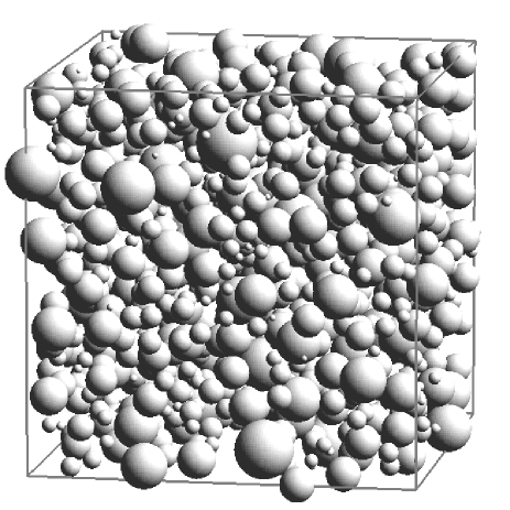
FIG. 5.: Zhang, Journal of Chemical Physics

FIG. 6.: Zhang, Journal of Chemical Physics

REFERENCES

- [1] J. J. Salacuse and G. Stell, J. Chem. Phys. 77, 3714 (1982).
- [2] R. J. Baxter, J. Chem. Phys. 52, 4559 (1970).
- [3] F. M. Reza, An introduction to Information Theory (Dover, New York, 1994).
- [4] J. A. Gualteri, J. M. Kincaid, and G. Morrison, J. Chem. Phys. 77, 521 (1982).
- [5] G. A. Mansoori, N. F. Carnahan, K. E. Starling, and T. W. Leland, J. Chem. Phys. 54, 1523 (1971).
- [6] D. Frenkel and B. Smit, Understanding Molecular Simulation:From Algorithms to Applications (Academic Press, San Diego, 1996).
- [7] G. Jackson, J. S. Rowlinson, and F. van Swol, J. Phys. Chem. 91, 4907 (1987).
- [8] D. Frenkel, R. J. Vos, C. G. de Kruif, and A. Vrij, J. Chem. Phys. 84, 4625 (1986).
- [9] W. G. T. Kranendonk and D. Frenkel, Mol. Phys. 72, 715 (1991).