Thermodynamics of the glassy state

Abstract

A picture for thermodynamics of the glassy state is introduced. It assumes that one extra parameter, the effective temperature, is needed to describe the glassy state. This explains the classical paradoxes concerning the Ehrenfest relations and the Prigogine-Defay ratio.

As a second part, the approach connects the response of macroscopic observables to a field change with their temporal fluctuations, and with the fluctuation-dissipation relation, in a generalized non-equilibrium way.

I Introduction

Non-equilibrium thermodynamics for systems far from equilibrium has long been a field of confusion. A typical application is window glass. Such a system is far from equilibrium: a cubic micron of glass is neither a crystal nor an ordinary under-cooled liquid. It is an under-cooled liquid that, in the glass formation process, has fallen out of its meta-stable equilibrium.

Until our recent works on this field, the general consensus reached after more than half a century of research was: Thermodynamics does not work for glasses, because there is no equilibrium Angell . This conclusion was mainly based on the failure to understand the Ehrenfest relations and the related Prigogine-Defay ratio. It should be kept in mind that, so far, the approaches leaned very much on equilibrium ideas. Well known examples are the 1951 Davies-Jones paper DaviesJones , the 1958 Gibbs-DiMarzio  GibbsDiMarzio and the 1965 Adam-Gibbs AdamGibbs papers, while a 1981 paper by DiMarzio has title “Equilibrium theory of glasses” and a subtitle “An equilibrium theory of glasses is absolutely necessary” DiMarzio1981 . We shall stress that such approaches are not applicable, due to the inherent non-equilibrium character of the glassy state.

Thermodynamics is the most robust field of physics. Its failure to describe the glassy state is quite unsatisfactory, since up to 25 decades in time can be involved. Naively we expect that each decade has its own dynamics, basically independent of the other ones. We have found support for this point in models that can be solved exactly. Thermodynamics then means a description of system properties under smooth enough non-equilibrium conditions.

II Thermodynamic picture for a system described by an effective temperature

A state that slowly relaxes to equilibrium is characterized by the time elapsed so far, sometimes called “age” or “waiting time”. For glassy systems this is of special relevance. For experiments on spin glasses it is known that non-trivial cooling or heating trajectories can be described by an effective age Hammann . Yet we do not wish to discuss spin glasses. They have an infinity of long time-scales, or infinite order replica symmetry breaking.

We shall restrict to systems with one diverging time scale, having, in the mean field limit, one step of replica symmetry breaking. They are systems with first-order-type phase transitions, with discontinuous order parameter, though usually there is no latent heat. (As we shall discuss, the same approach applies to true first order glassy transitions that do have a latent heat.)

We shall consider glassy transitions for glass forming liquids as well as for random magnets. The results map onto each other by interchanging volume $V$, pressure $p$, compressibility $\kappa=-\partial\ln V/\partial p$, and expansivity $\alpha=\partial\ln V/\partial T$, by magnetization $M$, field $H$, susceptibility $\chi=(1/N)\partial M/\partial H$, and “magnetizability” $\alpha=(-1/N)\partial M/\partial T$, respectively.

The picture to be investigated in this work starts by describing a non-equilibrium state characterized by three parameters, namely $T,p$ and the age $t$, or, equivalently, $T,p$ and the effective temperature $T_{e}(t)$. This quantity has to follow from solving the dynamics of the system, or from doing appropriate experiments. For a set of smoothly related cooling experiments $T_{i}(t)$ at pressures $p_{i}$, one may express the effective temperature as a continuous function: $T_{e,i}(t)$ $\to$ $T_{e}(T,p)$. This sets a surface in $(T,T_{e},p)$ space, that becomes multi-valued if one first cools, and then heats. For covering the whole space one needs to do many experiments, e.g., at different pressures and different cooling rates. The results should agree with findings from heating experiments and aging experiments. Thermodynamics amounts to giving differential relations between observables at nearby points in this space.

Of special importance is the thermodynamics of a thermal body at temperature $T_{2}$ in a heat bath at temperature $T_{1}=T$. This could apply to mundane situations such as a cup of coffee, or an ice-cream, in a room. There are also two entropies, $S_{1}$ and $S_{2}$. Notice that there are also two time-scales: the time-scale for heat to leave the cup is some ten minutes, while the time-scale for equilibrating that heat in the room is much smaller. This separation of time-scales allows the difference in temperatures. The change in heat of such a system obeys ${\mathchar 22\relax\mkern-11.0mu{\rm d}}Q\leq T_{1}{\rm d}S_{1}+T_{2}{\rm d}S_{2}$.

A similar two-temperature approach proves to be relevant for glassy systems. The known exact results on the thermodynamics of systems without currents can be summarized by the very same change in heat  NEhren Nthermo

$${\mathchar 22\relax\mkern-11.0mu{\rm d}}Q=T{\rm d}S_{\rm ep}+T_{e}{\rm d}{\cal I}$$ (1)

where $S_{\rm ep}$ is the entropy of the fast or equilibrium processes ($\beta$-processes) and ${\cal I}$ the configurational entropy of the slow or configurational processes ($\alpha$-processes). This object is also known as information entropy or complexity. In the standard definition GibbsDiMarzio the configurational entropy ${\cal I}$ is the entropy of the glass minus the one of the vibrational modes of the crystal. For polymers it still includes short-distance rearrangements, which is a relatively fast mode. It was confirmed numerically that ${\cal I}$ indeed does not vanish at any temperature, thus violating the Adam-Gibbs relation between timescale and configurational entropy Binder . In our definition the configurational entropy only involves long-time processes; the relatively fast ones are counted in $S_{\rm ep}$. With this point of view the applicability of the Adam-Gibbs relation remains an open issue.

It is both surprising and satisfactory that a glass can be described by the same general law. If, in certain systems, also an effective pressure or field would be needed, then ${\mathchar 22\relax\mkern-11.0mu{\rm d}}Q$ is expected to keep the same form, but ${\mathchar 22\relax\mkern-11.0mu{\rm d}}W$ would change from its standard value $-p{\rm d}V$ for liquids, or $-M{\rm d}H$ for magnets. In the latter case it would become $-M_{1}{\rm d}H-M_{2}{\rm d}H_{e}$, where $H_{e}$ is the effective field, and $M_{1}$ and $M_{2}$ add up to $M$. Such an extension could be needed to describe a larger class of systems.

II.1 First and second law

For a glass forming liquid the first law ${\rm d}U={\mathchar 22\relax\mkern-11.0mu{\rm d}}Q+{\mathchar 22\relax\mkern-11.0mu{\rm d}}W$ becomes

$${\rm d}U=T{\rm d}S_{\rm ep}+T_{e}{\rm d}{\cal I}-p{\rm d}V$$ (2)

It is appropriate to define the generalized free enthalpy

$$G = U-TS_{\rm ep}-T_{e}{\cal I}+pV$$ (3)

This is not the standard form, since $T_{e}\neq T$. It satisfies

$${\rm d}G = -S_{\rm ep}{\rm d}T-{\cal I}{\rm d}T_{e}+V{\rm d}p$$ (4)

The total entropy is

$$S=S_{\rm ep}+{\cal I}$$ (5)

The second law requires ${\mathchar 22\relax\mkern-11.0mu{\rm d}}Q\leq T{\rm d}S$, leading to

$$(T_{e}-T){\rm d}{\cal I}\leq 0,$$ (6)

which merely says that heat goes from high to low temperatures.

Since $T_{e}=T_{e}(T,p)$, and both entropies are functions of $T$, $T_{e}$ and $p$, the expression (1) yields a specific heat

$$C_{p} = \frac{\partial Q}{\partial T}{\Bigl{.}\Bigr{|}}_{p}=T(\frac{\partial S_{\rm ep}}{\partial T}{\Bigl{.}\Bigr{|}}_{T_{e},p}+\frac{\partial S_{\rm ep}}{\partial T_{e}}{\Bigl{.}\Bigr{|}}_{T,p}\frac{\partial T_{e}}{\partial T}{\Bigl{.}\Bigr{|}}_{p})+T_{e}(\frac{\partial{\cal I}}{\partial T}{\Bigl{.}\Bigr{|}}_{T_{e},p}+\frac{\partial{\cal I}}{\partial T_{e}}{\Bigl{.}\Bigr{|}}_{T,p}\frac{\partial T_{e}}{\partial T}{\Bigl{.}\Bigr{|}}_{p})$$ (7)

In the glass transition region all factors, except $\partial_{T}T_{e}$, are basically constant. This leads to

$$C_{p} = C_{1}+C_{2}\frac{\partial T_{e}}{\partial T}{\Bigl{.}\Bigr{|}}_{p}$$ (8)

Precisely this form has been assumed half a century ago by Tool Tool as starting point for the study of caloric behavior in the glass formation region, and has often been used for the explanation of experiments  DaviesJones Jaeckle86 . It is a direct consequence of eq. (1).

For magnetic systems the first law brings

$${\rm d}U = T{\rm d}S_{\rm ep}+T_{e}{\rm d}{\cal I}-M{\rm d}H$$ (9)

As above, one can define the free energy $F=U-TS_{\rm ep}-T_{e}{\cal I}$. It satisfies the relation ${\rm d}F=-S_{\rm ep}{\rm d}T-{\cal I}{\rm d}T_{e}-M{\rm d}H$.

II.2 Modified Maxwell relation

For a smooth sequence of cooling procedures of a glassy liquid, eq. (2) implies a modified Maxwell relation between macroscopic observables such as $U(t,p)\to U(T,p)=U(T,T_{e}(T,p),p)$ and $V$. This solely occurs since $T_{e}$ is a non-trivial function of $T$ and $p$ for the smooth set of experiments under consideration.

For glass forming liquids it reads

$$\frac{\partial U}{\partial p}{\Bigl{.}\Bigr{|}}_{T}+p\frac{\partial V}{\partial p}{\Bigl{.}\Bigr{|}}_{T}+T\frac{\partial V}{\partial T}{\Bigl{.}\Bigr{|}}_{p}=T\frac{\partial{\cal I}}{\partial T}{\Bigl{.}\Bigr{|}}_{p}\,\frac{\partial T_{e}}{\partial p}{\Bigl{.}\Bigr{|}}_{T}-T\frac{\partial{\cal I}}{\partial p}{\Bigl{.}\Bigr{|}}_{T}\,\frac{\partial T_{e}}{\partial T}{\Bigl{.}\Bigr{|}}_{p}+T_{e}\frac{\partial{\cal I}}{\partial p}{\Bigl{.}\Bigr{|}}_{T}$$ (10)

This is the modified Maxwell relation between observables $U$ and $V$. In equilibrium $T_{e}=T$, so the right hand side vanishes, and the standard form is recovered.

Similarly, one finds for a glassy magnet

$$\frac{\partial U}{\partial H}{\Bigl{.}\Bigr{|}}_{T}+M-T\frac{\partial M}{\partial T}{\Bigl{.}\Bigr{|}}_{H}=T_{e}\frac{\partial{\cal I}}{\partial H}{\Bigl{.}\Bigr{|}}_{T}+T\left(\frac{\partial T_{e}}{\partial H}{\Bigl{.}\Bigr{|}}_{T}\frac{\partial{\cal I}}{\partial T}{\Bigl{.}\Bigr{|}}_{H}-\frac{\partial T_{e}}{\partial T}{\Bigl{.}\Bigr{|}}_{H}\frac{\partial{\cal I}}{\partial H}{\Bigl{.}\Bigr{|}}_{T}\right)$$ (11)

II.3 Modified Clausius-Clapeyron relation

Let us consider a first order transition between two glassy phases A and B. An example could be the transition from low-density-amorphous ice to high-density-amorphous ice  LDAHDAice . For the standard Clausius-Clapeyron relation one uses that the free enthalpy $G$ is continuous along the first order phase transition line $p_{g}(T)$. Since $T_{e}\neq T$, it is actually not obvious that the function $G$ should still be continuous there. Based on a quasi-static approach involving a partition sum and, equivalently, on the experience that in mean field models replica theory has always brought the relevant physical free energy, we expect that our generalized free enthalpy (3) is indeed continuous at this transition.

Let us consider a first order transition between phases A and B. Assuming that $\Delta G=0$ along the glass transition line $p_{g}(T)$, a little amount of algebra yields the modified Clausius-Clapeyron relation

$$\Delta V\frac{{\rm d}p_{g}}{{\rm d}T}=\frac{\Delta U+p_{g}\Delta V}{T}+\Delta\left(\frac{{\rm d}T_{e}}{{\rm d}T}{\cal I}-\frac{T_{e}}{T}{\cal I}\right)$$ (12)

where ${\rm d}/{\rm d}T=\partial/\partial T+({\rm d}p_{g}/{\rm d}T)\partial/\partial p$ is the “total” derivative along the transition line.

It would be very interesting to test this relation for the two forms of amorphous ice. For those substances Mishima and Stanley HES have presented a thermodynamic construction of the standard free enthalpy or Gibbs potential $G$. It is, however, based on equilibrium ideas and, in contrast to eq. (3), does not involve the effective temperature in the amorphous phases. This approach therefore predicts the validity of the standard Clausius-Clapeyron relation. We feel that the standard $G$ is not the physically relevant one, and that the analysis should be redone, by considering many cooling rates and taking into account the effective temperature and the possible violation of the Clausius-Clapeyron relation by going from the high density amorphous phase to the low density one, and vice versa.

When phase A is an equilibrium under-cooled liquid, and phase B is a glass, it holds that $T_{e}=T$ in phase A. Then the relation reduces to

$$(V_{A}-V_{B})\frac{{\rm d}p_{g}}{{\rm d}T}=\frac{U_{A}-U_{B}+p_{g}(V_{A}-V_{B})}{T}+(\frac{T_{e}}{T}-\frac{{\rm d}T_{e}}{{\rm d}T}){\cal I}_{B}$$ (13)

Several models for magnets undergoing a first order glassy transitions with a latent heat have been studied in the literature  Mottishaw Goldschmidt ThirumDobrov NRitort .

II.4 Ehrenfest relations and Prigogine-Defay ratio

In the glass transition region a glass forming liquid exhibits smeared jumps in the specific heat $C_{p}$, the expansivity $\alpha$ and the compressibility $\kappa$. If one forgets about the smearing, one may consider them as true discontinuities, yielding an analogy with continuous phase transitions of the classical type.

Following Ehrenfest one may take the derivative of $\Delta V(T,p_{g}(T))=0$. The result for a glass forming liquid may be written as

$$\Delta\alpha=\Delta\kappa\frac{{\rm d}p_{g}}{{\rm d}T}$$ (14)

while for a glassy magnet

$$\Delta\alpha=\Delta\chi\frac{{\rm d}H_{g}}{{\rm d}T}$$ (15)

The conclusion drawn from half a century of research on glass forming liquids is that this relation is never satisfied  DaviesJones Goldstein Jaeckle  Angell . This has very much hindered progress on a thermodynamical approach. However, from a theoretical viewpoint it is hard to imagine that something could go wrong when just taking a derivative. We have pointed out that this relation is indeed satisfied automatically NEhren , but it is important say what is meant by $\kappa$ in the glassy state.

Let us make an analogy with spin glasses. In mean field theory they have infinite order replica symmetry breaking. From the early measurements of Canella and Mydosh  Mydoshboek on AuFe it is known that the susceptibility depends logarithmically on the frequency, so on the time scale. The short-time value, called Zero-Field-Cooled (ZFC) susceptibility is a lower bound, while the long time value, called Field-Cooled (FC) susceptibility is an upper bound. Let us use the term “glassy magnets” for spin glasses with one step of replica symmetry breaking. They are relevant for comparison with glass forming liquids. For them the situation is worse, as the ZFC value is discontinuous immediately below $T_{g}$. This explains why already directly below the glass transition different measurements yield different values for $\kappa$. These notions are displayed in figure 1.

Figure 1: Schematic plot of the field-cooled (FC) and zero-field-cooled (ZFC) susceptibility in realistic spin glasses and in glassy magnets, as function of temperature, in arbitrary units. In realistic spin glasses the infinite time or field-cooled susceptibility is larger than the short time or zero-field-cooled susceptibility. In magnetic analogs of realistic glasses the short time susceptibility even has a smeared discontinuity at the glass transition, yielding a value of $\chi$ that depends on the precise type of experiment which is performed. In glass forming liquids the same happens for the compressibility.

Previous claims about the violation of the first Ehrenfest relation can be traced back to the equilibrium thermodynamics idea that there is one, ideal $\kappa$, to be inserted in (14). Indeed, investigators always considered cooling curves $V(T,p_{i})$ at a set of pressures $p_{i}$ to determine $\Delta\alpha$ and ${\rm d}p_{g}/{\rm d}T$. However, $\Delta\kappa$ was always determined in another way, often from measurements of the speed of sound, or by making more complicated pressure steps RehageOels . In equilibrium such alternative determinations would yield the same outcome. In glasses this is not the case: the speed of sound is a short-time process, and additional pressure steps modify the glassy state. Therefore alternative procedures should be avoided, and only the cooling curves $V(T,p_{i})$ should be used. They constitute a liquid surface $V_{\rm liquid}(T,p)$ and a glass surface $V_{\rm glass}(T,p)$ in $(T,p,V)$ space. These surfaces intersect, and the first Ehrenfest relation is no more than a mathematical identity about the intersection line of these surfaces. It is therefore automatically satisfied NEhren . The most careful data we came across were collected by Rehage and Oels for atactic polystyreneRehageOels . In figure 2 we present those data in a 3-d plot, underlining our point of view.

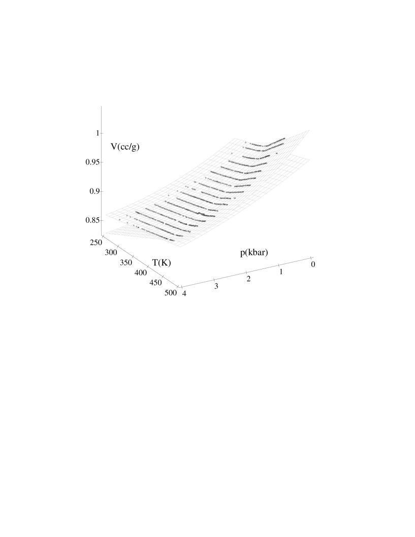
Figure 2: Data of the glass transition for cooling atactic polystyrene at rate 18 $K/h$, scanned from the paper of Rehage and Oels (1976): specific volume $V$ ($cm^{3}/g$) versus temperature $T$ ($K$) at various pressures $p$ ($k\,bar$). As confirmed by a polynomial fit, the data in the liquid essentially lie on a smooth surface, and so do the data in the glass. The first Ehrenfest relation describes no more than the intersection of these surfaces, and is therefore automatically satisfied. The values for the compressibility derived in this manner will generally differ from results obtained via other procedures.

The second Ehrenfest relation follows from differentiating $\Delta U(T,p_{g}(T))=0$. The obtained relation will also be satisfied automatically. However, one then eliminates $\partial U/\partial p$ by means of the Maxwell relation. We have already discussed that outside equilibrium it is modified. As a result we obtain

$$\frac{\Delta C_{p}}{T_{g}V} = \Delta\alpha\frac{{\rm d}p_{g}}{{\rm d}T}+\frac{1}{V}\left(1-\frac{\partial T_{e}}{\partial T}{\Bigl{.}\Bigr{|}}_{p}\right)\,\frac{{\rm d}{\cal I}}{{\rm d}T}$$ (16)

The ${\cal I}$ term constitutes the “total” derivative of the configurational entropy along the glass transition line. Its prefactor only vanishes at equilibrium, in which case the standard Ehrenfest relation is recovered.

For glassy magnets one has similarly

$$\frac{\Delta C}{NT}=\Delta\alpha\frac{{\rm d}H_{g}}{{\rm d}T}+\frac{1}{N}\left(1-\frac{\partial T_{e}}{\partial T}{\Bigl{.}\Bigr{|}}_{H}\right)\,\frac{{\rm d}{\cal I}}{{\rm d}T}$$ (17)

The equality $T_{e}(T,p_{g}(T))=T$ implies the resulting identity

$$\frac{{\rm d}T_{e}}{{\rm d}T}=\frac{\partial T_{e}}{\partial T}{\Bigl{.}\Bigr{|}}_{p}+\frac{\partial T_{e}}{\partial p}{\Bigl{.}\Bigr{|}}_{T}\frac{{\rm d}p_{g}}{{\rm d}T}=1$$ (18)

Combining the two Ehrenfest relations one may eliminate the slope of the transition line. This leads to the so-called Prigogine-Defay ratio

$$\Pi=\frac{\Delta C_{p}\Delta\kappa}{TV(\Delta\alpha)^{2}}$$ (19)

This looks like an equilibrium quantity. For equilibrium transitions it should be equal to unity. Assuming that at the glass transition a number of unspecified parameters undergo a phase transition, Davies and Jones derived that $\Pi\geq 1$ DaviesJones , while DiMarzio showed that in that case the correct value is $\Pi=1$  DiMarzio . In glasses typical experimental values are reported in the range $2<\Pi<5$. It was therefore generally expected that $\Pi\geq 1$ is a strict inequality arising from the requirement of mechanical stability.

We have pointed out, however, that, since the first Ehrenfest relation is satisfied, it holds that

$$\Pi=\frac{\Delta C_{p}}{TV\Delta\alpha({\rm d}p_{g}/{\rm d}T)}=1+\frac{1}{V\Delta\alpha}\left(1-\frac{\partial T_{e}}{\partial T}\Bigl{|}_{p}\Bigr{.}\right)\frac{{\rm d}{\cal I}}{{\rm d}p}$$ (20)

Depending on the smooth set of experiments to be performed, ${\rm d}p_{g}/{\rm d}T$ can be small or large: $\Pi$ depends on the set of experiments. As a result, it can also be below unity. Rehage-Oels found $\Pi=1.09\approx 1$ at $p=1$ $k\,bar$, using a short-time value for $\kappa$. Reanalyzing their data we find from (20), where the correct $\kappa$ has been inserted, a value $\Pi=0.77$, which indeed is below unity. The commonly accepted inequality $\Pi\geq 1$ is based on the equilibrium assumption of a unique $\kappa$. Our theoretical arguments and the Rehage-Oels data show that such idea’s are incorrect.

II.5 Fluctuation formula

The basic result of statistical physics is that it relates fluctuations in macroscopic variables to response of their averages to changes in external field or temperature. We have wondered whether such relations generalize to the glassy state. We have found arguments in favor of such a possibility both from the fluctuation-dissipation relation and by exactly solving the dynamics of model systems  Nhammer . Susceptibilities appear to have a non-trivial decomposition, that looks as being very general. Here we give arguments leading to it.

In cooling experiments at fixed field it holds that $M=$$M(T(t),T_{e}(t,H),H)$. For thermodynamics one eliminates time, implying $M=$$M(T,T_{e}(T,H),H)$. One may then expect two terms:

$$\chi \equiv \frac{1}{N}\,\frac{\partial M}{\partial H}\Bigl{|}_{T}\Bigr{.}=\chi^{\rm fluct}(t)+\chi^{\rm conf}(t)$$ (21)

The first is the fluctuation contribution

$$\chi^{\rm fluct}(t) = \frac{1}{N}\frac{\partial M}{\partial H}\Big{|}_{T,T_{e}}\Bigr{.}$$ (22)

To calculate it, we switch from a cooling experiment to an aging experiment at the considered $T$, $T_{e}$ and $H$, by keeping, in Gedanken, $T$ fixed from then on. The system will continue to age, expressed by $T_{e}=T_{e}(t;T,H)$. We may then use the equality

$$\frac{\partial M}{\partial H}\Big{|}_{T,t}\Bigr{.}=\frac{\partial M}{\partial H}\Big{|}_{T,T_{e}}\Bigr{.}+\frac{\partial M}{\partial T_{e}}\Big{|}_{T,H}\Bigr{.}\frac{\partial T_{e}}{\partial H}\Big{|}_{T,t}\Bigr{.}$$ (23)

We have conjectured  Nhammer that the left hand side may be written as the sum of fluctuation terms for fast and slow processes,

$$\frac{\partial M}{\partial H}\Big{|}_{T,t}\Bigr{.}=\frac{\langle\delta M^{2}(t)\rangle_{\rm fast}}{NT(t)}+\frac{\langle\delta M^{2}(t)\rangle_{\rm slow}}{NT_{e}(t)}$$ (24)

The first term is just the standard equilibrium expression for the fast equilibrium processes. Notice that the slow processes enter with their own temperature, the effective temperature. This decomposition is confirmed by use of the fluctuation-dissipation relation in the form to be discussed below. Combination of (22), (23) and (24) yields our non-equilibrium prediction

$$\chi^{\rm fluct}(t) = \frac{\langle\delta M^{2}(t)\rangle_{\rm fast}}{NT(t)}+\frac{\langle\delta M^{2}(t)\rangle_{\rm slow}}{NT_{e}(t)}-\frac{1}{N}\frac{\partial M}{\partial T_{e}}\Big{|}_{T,H}\,\,\frac{\partial T_{e}}{\partial H}\Bigr{|}_{T,t}$$ (25)

The first two terms are instantaneous, and thus the same for aging and cooling. The third term is a correction, related to an aging experiment. In the models considered so far, this term is small Nhammer Nlongthermo .

Since $T_{e}\neq T$, there occurs in eq. (21) also a new, configurational term

$$\chi^{\rm conf}=\frac{1}{N}\,\frac{\partial M}{\partial T_{e}}\Bigl{|}_{T,H}\,\,\frac{\partial T_{e}}{\partial H}\Bigr{|}_{T}$$ (26)

It originates from the difference in the system’s structure for cooling experiments at nearby fields. This is the term that is responsible for the discontinuity of $\chi$ at the glass transition. For glass forming liquids such a term occurs in the compressibility. Its existence was anticipated in some earlier work Goldstein  Jaeckle .

II.6 Fluctuation-dissipation relation

Nowadays quite some attention is payed to the fluctuation-dissipation relation in the aging regime of glassy systems. It was first put forward in works by Horner Horner1 CHS and generalized by Cugliandolo and Kurchan, see  BCKM for a review.

In the aging regime there holds a fluctuation-dissipation relation between the correlation function $C(t,t^{\prime})$$=$$<\!\delta M(t)\delta M(t^{\prime})\!>$ and $G(t,t^{\prime})$, the response of $<\!M(t)\!>$ to a short, small field change $\delta H(t^{\prime})$ applied at an earlier time $t^{\prime}$,

$$\frac{\partial C(t,t^{\prime})}{\partial t^{\prime}}=T_{e}(t,t^{\prime}){G(t,t^{\prime})}$$ (27)

with $T_{e}(t,t^{\prime})$ being an effective temperature, formally defined by this relation. In the equilibrium or short-time regime $|t-t^{\prime}|\ll t$, it is just equal to $T$; in the aging regime $t/t^{\prime}={\cal O}(1)$, it depends only logarithmically on $t$ and $t^{\prime}$, making it a useful concept.

We have observed that in simple models without fast processes $T_{e}(t,t^{\prime})=\tilde{T}_{e}(t^{\prime})$ is a function of one of the times only. One then expects that $\tilde{T}_{e}(t)$ is close to the “thermodynamic” effective temperature $T_{e}(t)$. We have shown that  Nlongthermo

$$\tilde{T}_{e}(t)=T_{e}(t)-\dot{T}_{e}(t)\left(\frac{\partial\ln C(t,t^{\prime})}{\partial t^{\prime}}{\Bigl{.}\Bigr{|}}_{t^{\prime}=t}\right)^{-1}+\cdots$$ (28)

So the effective temperatures $T_{e}$ and $\tilde{T}_{e}$ are not identical. However, in the models analyzed so far, the difference is subleading in $1/\ln t$.

Notice that the ratio $\partial_{t^{\prime}}C(t,t^{\prime})/G(t,t^{\prime})=\tilde{T}_{e}(t^{\prime})$ is allowed to depend on time $t^{\prime}$. The situation with constant $T_{e}$ is well known from mean field spin glasses BCKM , but we have not found such a constant $T_{e}$ beyond mean-field Nhammer Nlongthermo . Only at exponential time-scales the mean field spin glass behaves as a realistic system Nthermo .

II.7 Time-scale arguments

Consider a simple system that has only one type of processes ($\alpha$ processes), which falls out of equilibrium at some low $T$. When it ages a time $t$ at $T=0$ it will have achieved a state with effective temperature $T_{e}$, that can be estimated by equating time with the equilibrium time-scale. Let us define ${\overline{T}}_{e}$ by

$$t=\tau_{eq}({\overline{T}}_{e})$$ (29)

We have checked in solvable models that, to leading order in $\ln t$, it holds that ${\overline{T}}_{e}=T_{e}$. (The first non-leading order turns out to be non-universal). This equality also is found in cooling trajectories, when the system is well inside the glassy regime. It says that the system basically has forgotten its history, and ages on its own, without caring about the actual temperature. Another way of saying is that dynamics in each new time-decade is basically independent of previous decade.

In less trivial systems, for instance those having a Vogel-Tammann-Fulcher law, the time-scale may have parameters that depend on the actual temperature, implying $\tau=\tau(T,T_{e})$. We have already found support for the expectation that, to leading order, $T_{e}$ follows by equating this expression with time $t$.

In many systems one finds a $t^{\prime}/t$ scaling in the aging regime of two-time quantities. There is a handwaving argument to explain that:

$$C(t,t^{\prime})\approx C(\frac{t-t^{\prime}}{\tau_{eq}(T_{e}(t^{\prime}))})\approx C(\frac{t-t^{\prime}}{t^{\prime}})=C(\frac{t}{t^{\prime}})$$ (30)

showing indeed the familiar $t/t^{\prime}$ scaling. In the models studied so far we have found logarithmic scaling corrections  Nhammer Nlongthermo .

III Solvable models

The above relations have been tested in models of which the statics is exactly solvable, and the dynamics is partially solvable, such as the $p$-spin model CHS NEhren and a directed polymer model with glassy behavior  Ndirpol NEhren . Partial results follow from the backgammon model FranzRitort , GodrecheLuck .

More interesting are models with exactly solvable parallel Monte Carlo dynamics, such as independent harmonic oscillators BPR  Nhammer Nlongthermo or independent spherical spins in a random field  Nhammer Nlongthermo . In both cases a glassy behavior occurs when cooling towards low temperatures. A related model with a set of fast modes and a set of slow modes, that have a Vogel-Fulcher-Tammann-Hesse law for the divergence of the equilibrium time-scale, is currently under study.

The two-temperature approach put forward here also explains the thermodynamics of black holes Nblackhole and star clusters Nstarcl .

References

- (1) Angell C.A., Science 267 1924 (1995)
- (2) Davies R.O. and G.O. Jones G.O., Adv. Phys. 2 370 (1953)
- (3) Gibbs J.H. and DiMarzio E.A., J. Chem. Phys. 28 373 (1958)
- (4) Adam G. and Gibbs J.H., J. Chem. Phys. 43 139 (1965)
- (5) DiMarzio E.A., Ann. NY Acad. Sci. 371 1 (1981)
- (6) Lefloch F., Hammann J., Ocio M., and Vincent E., Europhys. Lett. 18 647 (1992)
- (7) Nieuwenhuizen Th.M. , Phys. Rev. Lett. 79 1317 (1997)
- (8) Nieuwenhuizen Th.M., J. Phys. A 31 L201 (1998)
- (9) Wolfgardt M., Baschnagel J., Paul W., and Binder K., Phys. Rev. E 54 1535 (1996)
- (10) Tool A.Q., J. Am. Ceram. Soc. 29 240 (1946)
- (11) Jäckle J, Rep. Prog. Phys. 49 171 (1986)
- (12) Mishima O., Calvert L.D. and Whalley E., Nature 314 76 (1985)
- (13) Mishima O. and Stanley H.E., Nature 392 164 (1998)
- (14) Mottishaw P., Europhys. Lett. 1 409 (1986)
- (15) Goldschmidt Y.Y., Phys. Rev. B 41 4858 (1990)
- (16) Dobrosavljevic V. and Thirumalai D., J. Phys. A 22 L767 (1990)
- (17) Nieuwenhuizen Th.M. and Ritort F., Physica A 250 8 (1998)
- (18) Goldstein M., J. Phys. Chem. 77 667 (1973)
- (19) Jäckle J., J. Phys: Condens. Matter 1 267 (1989): eq. (9)
- (20) Mydosh J.A., Spin glasses: an experimental introduction (Taylor and Francis, London, 1993)
- (21) Rehage G. and Oels H.J., High Temperatures-High Pressures 9 545 (1977)
- (22) DiMarzio E.A., J. Appl. Phys. 45 4143 (1974)
- (23) Nieuwenhuizen Th.M., Phys. Rev. Lett. 80 5580 (1998)
- (24) Nieuwenhuizen Th.M., submitted to Phys. Rev. E; cond-mat/9807161
- (25) Horner H., Z. Phys. B 86 291 (1992); ibid. 87 371 (1992)
- (26) Crisanti A. , Horner H., and Sommers H.J., Z. Phys. B 92 257 (1993)
- (27) Bouchaud J.P., Cugliandolo L.F., Kurchan J., and Mézard M., Physica A 226 243 (1996)
- (28) Nieuwenhuizen Th.M., Phys. Rev. Lett. 78 3491 (1997)
- (29) Franz S. and Ritort F., J. Phys. A 30 L359 (1997)
- (30) Godrèche C. and Luck J.M., J. Phys. A 30 6245 (1997)
- (31) Bonilla L.L., Padilla F.G., and Ritort F., Physica A 250 315 (1998)
- (32) Nieuwenhuizen Th.M., Phys. Rev. Lett. 81 2201 (1998)
- (33) Nieuwenhuizen Th.M., Do star clusters satisfy the second law of thermodynamics ?, preprint 1998