Aperiodic extended surface perturbations in the Ising model

Abstract

We study the influence of an aperiodic extended surface perturbation on the surface critical behaviour of the two-dimensional Ising model in the extreme anisotropic limit. The perturbation decays as a power $\kappa$ of the distance $l$ from the free surface with an oscillating amplitude $A_{l}\!=\!(-1)^{f_{l}}$ where $f_{l}\!=\!0,1$ follows some aperiodic sequence with an asymptotic density equal to $1/2$ so that the mean ampltitude vanishes. The relevance of the perturbation is discussed by combining scaling arguments of Cordery and Burkhardt for the Hilhorst-van Leeuwen model and Luck for aperiodic perturbations. The relevance-irrelevance criterion involves the decay exponent $\kappa$, the wandering exponent $\omega$ which governs the fluctuation of the sequence and the bulk correlation length exponent $\nu$. Analytical results are obtained for the surface magnetization which displays a rich variety of critical behaviours in the $(\kappa,\omega)$-plane. The results are checked through a numerical finite-size-scaling study. They show that second-order effects must be taken into account in the discussion of the relevance-irrelevance criterion. The scaling behaviours of the first gap and the surface energy are also discussed.

1 Introduction

At the free surface of a homogeneous $d$-dimensional sytem with short-range interactions displaying a bulk second-order phase transition, the scaling dimension $x_{\rm e}^{\rm s}$ of the surface energy density is equal to $d$ burkhardt87 . As a consequence, a weak short-range surface perturbation $\Delta K_{\rm s}$ of the reduced interaction $K\!=\!\beta J\!=\!J/k_{\rm B}T$ cannot change the surface critical behaviour, since its scaling dimension $y_{\Delta K}\!=\!d-1-x_{\rm e}^{\rm s}\!=\!-1$ and the perturbation is irrelevant. Such a pertubative argument does not exclude the occurence in $d\!>\!2$ dimensions of special, extraordinary, and surface transitions for strong enough enhancement of the surface couplings binder83 .

The situation is somewhat different for the Hilhorst-van Leeuwen (HvL) model hilhorst81 , in which the surface perturbation extends into the bulk of the system, decaying as a power of the distance $l$ from the surface with:

$$\Delta K(l)=\frac{A}{l^{\kappa}}\,.$$ (1.1)

Such extended surface perturbations may change the surface critical behaviour for an arbitrarily small value of the perturbation amplitude $A$. This can be explained cordery82 by noticing that, under a length scale transformation $l^{\prime}\!=\!l/b$, the extended thermal perturbation in (1.1) transforms as:

$$[\Delta K(l)]^{\prime}=\frac{A^{\prime}}{{l^{\prime}}^{\kappa}}=b^{1/\nu}\frac{A}{l^{\kappa}}\,,$$ (1.2)

so that, comparing both sides of the last equation, the perturbation amplitude scales as:

$$A^{\prime}=b^{-\kappa+1/\nu}\,A\,.$$ (1.3)

When the decay is strong enough ($\kappa\!>\!1/\nu$), the perturbation is irrelevant: it does not affect the surface critical behaviour. When $\kappa\!<\!1/\nu$, the perturbation is relevant: the decay is sufficiently slow to modify the surface critical behaviour. In the marginal situation, $\kappa\!=\!1/\nu$, one expects a nonuniversal surface critical behaviour.

Analytical results obtained for the two-dimensional ($2d$) Ising model, with $\nu\!=\!1$, are in complete agreement with these predictions blote83 ; hvl :

i) For $\kappa\!>\!1$, the scaling dimensions of the surface magnetization and the surface energy density are $x_{\rm m}^{\rm s}\!=\!1/2$ and $x_{\rm e}^{\rm s}\!=\!2$, respectively, like in the homogeneous semi-infinite system.

ii) In the marginal case, $\kappa\!=\!1$, when $A$ is smaller than a critical value $A_{\rm c}$, the surface transition is second-order with continuously varying surface scaling dimensions $x_{\rm m}^{\rm s}(A)$ and $x_{\rm e}^{\rm s}(A)$. For $A\!>\!A_{\rm c}$, the transition is first-order: there is a nonvanishing spontaneous surface magnetization at the bulk critical point which vanishes above $T_{\rm c}$ since the surface is one-dimensional.

iii) For $\kappa\!<\!1$, the surface transition is first-order for $A\!>\!0$ and continuous for $A\!<\!0$ where the surface magnetization displays an essential singularity.

In the present work we study an aperiodic version of the HvL model where the amplitude of the decay is modulated according to some aperiodic sequence. More specifically, we consider a layered semi-infinite system with constant reduced interactions $K_{1}\!=\!\beta J_{1}$ between nearest neighbours in the directions parallel to the free surface while the reduced interactions in the perpendicular direction are modulated and reads:

$$K_{2}(l)=K_{2}+\frac{A_{l}}{l^{\kappa}}\,,\qquad A_{l}=(-1)^{f_{l}}\,A\,,$$ (1.4)

where $f_{l}$ is aperiodic and takes the values 0 or 1. The aperiodic sequence is assumed to have equal densities of 0 and 1, such that the mean amplitude vanishes. Otherwise, the critical behaviour would be the same as for the HvL model with $A$ replaced by the average of the modulation amplitude $A_{l}$.

A relevance-irrelevance criterion will be proposed, which is a combination of the arguments of Burkhardt and Cordery for HvL perturbations cordery82 and those of Luck for aperiodic systems luck93 .

In Section 2, we recall the main results about the fluctuation properties of aperiodic sequences generated via substitutions and derive a relevance-irrelevance criterion for aperiodic HvL perturbations, which is valid to linear order in the perturbation amplitude. In Section 3, we examine the critical behaviour of the surface magnetization in the aperiodic HvL Ising quantum chain. The results of Section 3 are confronted to numerical data obtained via finite-size scaling (FSS) for different aperiodic sequences in Section 4. The influence of higher-order terms on the relevance of the perturbation, the scaling behaviours of the first gap and the surface energy are discussed in Section 5. Technical details are given in Appendices A and B.

2 Fluctuation of the perturbation amplitude and relevance-irrelevance criterion

We consider the aperiodic HvL model defined in (1.4) for a $d$-dimensional semi-infinite system with a bulk correlation length exponent $\nu$. The modulation of the perturbation amplitude follows some aperiodic sequence which can be generated through substitution rules queffelec87 .

Working with a finite alphabet $A$, $B$, $C$, … and starting for example with $A$, an infinite sequence of letters is obtained by first substituting a finite word $S(A)$ for $A$ and then iterating the process (with $B\to S(B)$, $C\to S(C)$, …). The required aperiodic sequence of digits $f_{l}$ is finally obtained by replacing each of the letters by a corresponding finite sequence of digits 0 and 1.

The information about the properties of the sequence is contained into the substition matrix with entries $n_{ij}$ giving the numbers of letters $i$ in $S(j)$ ($i$, $j\!=\!A$, $B$, $C$, …). Let $V_{\alpha}$ be the right eigenvectors of the substitution matrix and $\Lambda_{\alpha}$ the corresponding eigenvalues. The leading eigenvalue, $\Lambda_{1}$, is related to the dilatation factor $b$ of the self-similar sequence and gives its length after $n$ substitutions through $L_{n}\sim\Lambda_{1}^{n}$.

The asymptotic densities of letters $i\!=\!A$, $B$, $C$, … are related to the components of the eigenvector corresponding to the leading eigenvalue through:

$$\rho_{\infty}(i)=\frac{V_{1}(i)}{\sum_{j}V_{1}(j)}\,,$$ (2.1)

which allows a calculation of $\rho_{\infty}$, the asymptotic density of 1 in the sequence of digits $f_{l}$.

The sum of the digits $n_{l}\!=\!\sum_{k=1}^{l}f_{k}$ is such that:

$$n_{l}-l\rho_{\infty}\sim l^{\omega}\,,$$ (2.2)

with an amplitude which is log-periodic, i.e., a periodic function of $\ln l/\ln b$. The exponent

$$\omega=\frac{\ln|\Lambda_{2}|}{\ln\Lambda_{1}}$$ (2.3)

is the wandering exponent of the sequence. When $\omega\!<\!0$($>\!0$) the sequence has bounded (unbounded) fluctuations.

Using (2.2) and the identity

$$(-1)^{f_{k}}=1-2f_{k}\,,$$ (2.4)

the amplitude of the aperiodic HvL perturbation in (1.4), averaged at a length scale $l$, can be written as:

$$\overline{A}(l)=\frac{A}{l}\sum_{k=1}^{l}(-1)^{f_{k}}=A(1-2\frac{n_{l}}{l})\sim Al^{\omega-1}\,,$$ (2.5)

when the asymptotic density of 1 is $\rho_{\infty}\!=\!1/2$.

To analyse the relevance of the perturbation, one may replace $A_{l}$ by $Al^{\omega-1}$ in (1.4), which leads to the following behaviour under rescaling:

$$[\Delta K_{2}(l)]^{\prime}=\frac{A^{\prime}}{{l^{\prime}}^{\kappa-\omega+1}}=b^{1/\nu}\frac{A}{l^{\kappa-\omega+1}}\,,$$ (2.6)

or, for the perturbation amplitude:

$$A^{\prime}=b^{-\kappa+\omega-1+1/\nu}A\,.$$ (2.7)

Thus, to the first order in the amplitude, the perturbation is relevant (irrelevant) when $\kappa\!<\!(>)\omega-1+1/\nu$. Nonuniversal surface critical behaviour is expected in the marginal situation where $\kappa\!=\!\omega-1+1/\nu$.

For the Ising model in $2d$, $\nu\!=\!1$, and the relevance of the aperiodic HvL perturbation is simply governed by the sign of $\omega-\kappa$.

One may notice that Luck’s criterion for aperiodic perturbations luck93 is recovered when $\kappa\!=\!0$, which corresponds to an aperiodic modulation with a constant amplitude.

3 Surface magnetization of the Ising quantum chain: analytical approach

In this section, we study the critical behaviour of the surface magnetization for the $2d$ Ising model with an aperiodic extended surface perturbation given by (1.4).

3.1 Ising quantum chain in a transverse field

We work in the extreme anisotropic limit kogut79 where $K_{1}\to\infty$, $K_{2}(l)\to 0$, $A\to 0$, while the ratios

$$\lambda=K_{2}/K_{1}^{*}\,,\qquad a=A/K_{2}\,,$$ (3.1)

are kept fixed. The dual interaction $K_{1}^{*}\!=\!-1/2\ln(\tanh K_{1})$ enters into the expression of the unperturbed coupling $\lambda$.

In the extreme anisotropic limit, the row-to-row transfer operator, ${\cal T}\!=\!\exp(-2K_{1}^{*}{\cal H})$, involves the Hamiltonian of the quantum Ising chain in a transverse field kogut79 ; pfeuty70 :

$${\cal H}=-\frac{1}{2}\sum_{l=1}^{\infty}(\lambda_{l}\,\sigma_{l}^{z}\sigma_{l+1}^{z}+\sigma_{l}^{x})\,.$$ (3.2)

The ${\bf\sigma}$s are Pauli spin operators and the inhomogeneous couplings $\lambda_{l}$ take the HvL form:

$$\lambda_{l}=\lambda\left(1+\frac{a_{l}}{l^{\kappa}}\right)\,,\qquad a_{l}=(-1)^{f_{l}}a\,,$$ (3.3)

where $a_{l}$ is the aperiodic amplitude and $a$ is related to original parameters as indicated in (3.1). $\lambda$ plays the role of an inverse temperature and the deviation from the critical point, $\lambda_{\rm c}\!=\!1$, is measured by

$$t=1-\lambda^{-2}\,,$$ (3.4)

so that $0\!<\!t\!<\!1$ in the ordered phase.

Using the Jordan-Wigner transformation jordan28 and a canonical transformation of the fermion operators, the Hamiltonian can be put into diagonal form pfeuty70 ; lieb61 :

$${\cal H}=\sum_{\alpha}\epsilon_{\alpha}\left(\eta_{\alpha}^{\dagger}\eta_{\alpha}-\frac{1}{2}\right)\,,$$ (3.5)

where $\eta_{\alpha}^{\dagger}$ ($\eta_{\alpha}$) creates (destroys) a fermionic excitation. The excitation energies $\epsilon_{\alpha}$ are obtained by solving the following eigenvalue problem:

$$\lambda_{l-1}\phi_{\alpha}(l\!-\!1)+(1+\lambda_{l-1}^{2})\phi_{\alpha}(l)+\lambda_{l}\phi_{\alpha}(l\!+\!1)=\epsilon_{\alpha}^{2}\phi_{\alpha}(l)\,.$$ (3.6)

The physical properties of the system can be expressed in terms of the excitations $\epsilon_{\alpha}$ and the eigenvectors $\boldsymbol{\phi}_{\alpha}$ which are assumed to be normalized in the following.

3.2 Surface magnetization

The surface magnetization $m_{\rm s}$ is given by the matrix element $\langle 0|\sigma_{1}^{z}|\sigma\rangle$, where $|0\rangle$ is the vacuum state and $|\sigma\rangle$ is the lowest one-particle state $\eta_{1}^{\dagger}|0\rangle$. Expressing $\sigma_{1}^{z}$ in terms of diagonal fermion operators, one obtains $m_{s}\!=\!\phi_{1}(1)$, which can be simply evaluated noticing that the first excitation $\epsilon_{1}\!=\!0$ in the ordered phase peschel84 . This leads to:

$$m_{\rm s}=S^{-1/2}\,,\qquad S=1+\sum_{j=1}^{\infty}\prod_{l=1}^{j}\lambda_{l}^{-2}\,.$$ (3.7)

Using (3.3), the sum can be rewritten as:

$$S=1+\sum_{j=1}^{\infty}\lambda^{-2j}P_{j}^{-2}\,,\quad P_{j}=\prod_{l=1}^{j}\left[1+a\,\frac{(-1)^{f_{l}}}{l^{\kappa}}\right]\,.$$ (3.8)

Since the critical behaviour is governed by the long distance properties of the sytem, when $\kappa\!>\!0$, one may write:

$$\ln P_{j} = \sum_{l=1}^{j}\ln\left[1+a\,\frac{(-1)^{f_{l}}}{l^{\kappa}}\right]$$ (3.9)

$$\simeq \sum_{l=1}^{j}\left[a\,\frac{(-1)^{f_{l}}}{l^{\kappa}}-\frac{a^{2}}{2l^{2\kappa}}+(-1)^{f_{l}}O(l^{-3\kappa})\right].$$

To go further we need some approximate expression for $f_{l}$. Eqs. (2.2) and (2.5) suggest that, inside a sum, $f_{l}$ may be replaced by

$$f_{l}\simeq\rho_{\infty}+c(l)\,l^{\omega-1}\,,$$ (3.10)

where $c(l)$ is a log-periodic amplitude. Making use of the identity (2.4), with $\rho_{\infty}\!=\!1/2$, the first sum in the last equation of (3.9) can be rewritten as:

$$\sum_{l=1}^{j}\frac{(-1)^{f_{l}}}{l^{\kappa}}\simeq-2\sum_{l=1}^{j}c(l)\,l^{\omega-\kappa-1}=-2c_{\kappa}(j)\sum_{l=1}^{j}l^{\omega-\kappa-1}\,.$$ (3.11)

In the following, we assume that

$$c_{\kappa}(j)=\frac{\sum_{l=1}^{j}c(l)\,l^{\omega-\kappa-1}}{\sum_{l=1}^{j}l^{\omega-\kappa-1}}=\frac{\sum_{l=1}^{j}(f_{l}-1/2)l^{-\kappa}}{\sum_{l=1}^{j}l^{\omega-\kappa-1}}$$ (3.12)

can be replaced by some constant effective value $\overline{c}$ when $j\gg 1$ (see Appendix A for a discussion of the asymptotic properties of $c_{\kappa}(j)$).

Finally, when $\rho_{\infty}\!=\!1/2$ and $\kappa\!>\!0$, one obtains:

$$\ln P_{j}\simeq-\sum_{l=1}^{j}\left[\frac{2\overline{c}a}{l^{1-\omega+\kappa}}+\frac{a^{2}}{2l^{2\kappa}}+O(l^{-3\kappa+\omega-1})\right],$$ (3.13)

where the size of the leading omitted term follows from a comparison to the first one. Otherwise, when $\overline{a}_{l}\neq 0$, an additional term of order $l^{-\kappa}$ gives the leading contribution to the sum since $\omega\!<\!1$. As mentioned previously, the critical behaviour would then be the same as for the HvL model.

3.2.1 Relevant perturbations

We first consider the case of relevant perturbations which, according to the criterion of Section 2, corresponds to $\kappa\!<\!\omega$.

In Eq. (3.13) the first term dominates when $1-\omega+\kappa\!<\!2\kappa$, i.e., when $1-\omega\!<\!\kappa\!<\!\omega$, which can be satisfied only when $\omega\!>\!1/2$. Details about the calculation of the $t$-dependence of $m_{\rm s}$ and its finite-size behaviour at $\lambda_{\rm c}$ are given in Appendix B.

The surface critical behaviour depends on the sign of $\overline{c}a$. When $\overline{c}a\!>\!0$, the transition is continuous and the surface magnetization displays an essential singularity as a function of $t$:

$$m_{\rm s}(t) \sim \exp\left[-C\,t^{-(\omega-\kappa)/(\kappa-\omega+1)}\right]\,,$$

$$C = \frac{\kappa-\omega+1}{2(\omega-\kappa)}(\overline{c}a)^{1/(\kappa-\omega+1)}\,.$$ (3.14)

The finite-size behaviour at the critical point is the following:

$$m_{\rm s,c}(L)\sim\exp\left[-\frac{2\overline{c}a}{\omega-\kappa}\,L^{\omega-\kappa}\right]\,.$$ (3.15)

When $\overline{c}a\!<\!0$ the surface remains ordered at the bulk critical point, the transition is first-order and the surface magnetization approaches its critical value linearly in $t$.

The two terms in (3.13) give contributions of the same order to the sum when $\kappa\!=\!1-\omega$. As shown in Appendix B, when $\kappa\!<\!1/2$ the surface critical behaviour is modified and depends on the sign of $4\overline{c}a+a^{2}$. When $\overline{c}a\!<\!-4\overline{c}^{2}$ or $\overline{c}a\!>\!0$, the surface magnetization vanishes continuously with an essential singularity:

$$m_{\rm s}(t)\sim\exp\left[-\frac{\kappa}{1-2\kappa}(4\overline{c}a+a^{2})^{1/2\kappa}\,t^{1-1/2\kappa}\right]\,,$$ (3.16)

and:

$$m_{\rm s,c}(L)\sim\exp\left[-\frac{4\overline{c}a+a^{2}}{2(1-2\kappa)}\,L^{1-2\kappa}\right]\,.$$ (3.17)

When $-4\overline{c}^{2}\!<\!\overline{c}a\!<\!0$, as above the surface is ordered at the bulk critical point and the surface transition is first-order.

The second term of the sum in (3.13), involving $a^{2}$, is the dominant one if $\kappa\!<\!1-\omega$. As shown in Appendix B, this term becomes dangerous as soon as $\kappa\!<\!1/2$. When $\kappa\!>\!0$, it leads to an essential singularity for the surface magnetization with:

$$m_{\rm s}(t)\sim\exp\left[-\frac{\kappa|a|^{1/\kappa}}{1-2\kappa}\,t^{1-1/2\kappa}\right]$$ (3.18)

and

$$m_{\rm s,c}(L)\sim\exp\left[-\frac{a^{2}}{2(1-2\kappa)}\,L^{1-2\kappa}\right]\,.$$ (3.19)

The case $\kappa\!=\!1/2\!<\!1-\omega$, where the dangerous term leads to a marginal behaviour, will be examined in the next section.

One may notice that the surface critical behaviour is modified by the term in $a^{2}$ even when $\omega\!<\!\kappa\leq 1/2$, i.e., when the perturbation is irrelevant according to the criterion (2.7). Clearly this relevance-irrelevance criterion only concerns the contribution of the first term which is linear in $a$.

3.2.2 Marginal perturbations

According to the linear criterion of Section 2, the aperiodic HvL perturbation is expected to be marginal when $\kappa\!=\!\omega$. But we shall see that this is the actual behaviour only when $\omega\geq 1/2$.

For $\kappa\!=\!\omega\!>\!1/2$, the first term of the sum in (3.13) is the dominant one. When $\overline{c}a\!>\!-1/4$, as shown in Appendix B, this term leads to a second-order surface transition where $m_{\rm s}$ vanishes as $t^{\beta_{\rm s}}$ or, at the critical point, as $L^{-x_{\rm m}^{\rm s}}$. Since $\nu\!=\!1$, here and in what follows, both exponents have the same expression:

$$\beta_{\rm s}=x_{\rm m}^{\rm s}=\frac{1}{2}(1+4\overline{c}a)\,,$$ (3.20)

When $\overline{c}a\!<\!-1/4$, the transition is first-order and the approach to the critical surface magnetization is governed by the exponents ${\beta^{\prime}}_{\rm s}\!=\!{x^{\prime}}_{\rm m}^{\rm s}$ with

$$\beta^{\prime}_{\rm s}=-2\beta_{\rm s}(a)=-1-4\overline{c}a\,,$$ (3.21)

where $\beta_{\rm s}(a)$ is the continuation of $\beta_{\rm s}$ in the first-order region.

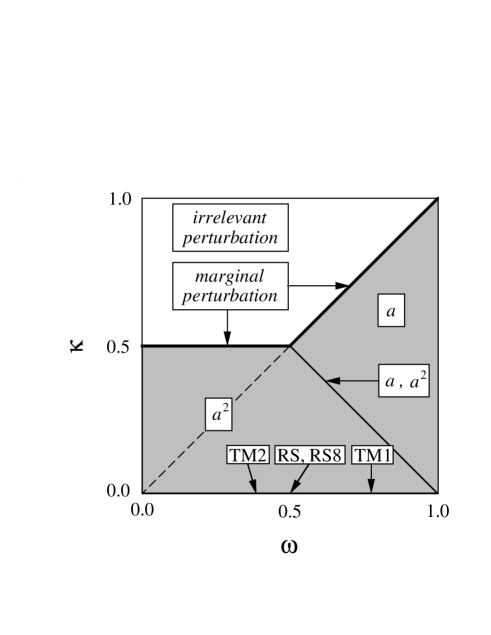
Figure 1: Relevance-irrelevance of aperiodic extended surface perturbations in the Ising quantum chain. The perturbation is relevant in the shaded region. To first order in the amplitude $a$, the perturbation is relevant only below the first diagonal. Below the second diagonal and the line $\kappa\!=\!1/2$ the second-order term is relevant and dominates the first-order one. On the marginal border line, the magnetization exponent is a function of $a$ above $\omega\!=\!1/2$, of $a^{2}$ below, and involves both terms at $\omega\!=\!1/2$. The values of $\omega$ for the aperiodic sequences used in the numerical FSS study are indicated.

For $\kappa\!=\!\omega\!=\!1/2$, the two terms in (3.13) are of the same order $l^{-1}$. Thus one obtains a second-order surface transition with

$$\beta_{\rm s}=\frac{1}{2}(1+4\overline{c}a+a^{2})$$ (3.22)

for values of $a$ leading to a non-negative expression, i.e., when $\overline{c}^{2}\!<\!1/4$ for any $a$ and when $\overline{c}^{2}\!>\!1/4$ for $a\!<\!-2\overline{c}\!-\!\Delta$ or $a\!>\!-2\overline{c}\!+\!\Delta$ where $\Delta\!=\!(4\overline{c}^{2}\!-\!1)^{1/2}$.

When $\overline{c}^{2}\!>\!1/4$, there is a first-order surface transition on the interval $-2\overline{c}\!-\!\Delta\!<\!a\!<\!-2\overline{c}\!+\!\Delta$ where $m_{\rm s}$ approaches its critical value as a power of $t$ or $L^{-1}$ with an exponent

$$\beta^{\prime}_{\rm s}=-2\beta_{\rm s}(a)=-1-4\overline{c}a-a^{2}\,.$$ (3.23)

As mentioned above, the second term in (3.13) is the dominant one and leads to a stretched exponential surface magnetization in the region $\kappa\!<\!1-\omega$, $\kappa\!<\!1/2$. The marginal line $\kappa\!=\!\omega$ of the linear relevance-irrelevance criterion is actually moved to $\kappa\!=\!1/2$ when $\omega\!<\!1/2$. On this line, the surface transition is second-order with (see Appendix B):

$$\beta_{\rm s}=\frac{1}{2}(1+a^{2})\,.$$ (3.24)

The behaviour in the $(\kappa,\omega)$-plane is recapitulated in Fig. 1. Notice that on the line $\kappa\!=\!0$ the bulk is homogeneously aperiodic and, according to the Luck criterion in Eq. (2.7), the perturbation is marginal at $\omega\!=\!0$. This marginal behaviour has been indeed confirmed by various exact results for aperiodic Ising models turban94 ; igloi97 ).

In Fig. 1 this point belongs to the domain of relevant perturbations due to terms of order $a^{2}$. This only means that the non-decaying aperiodicity changes the critical coupling from $\lambda_{\rm c}\!=\!1$ to $\lambda_{\rm c}\!=\!(1-a^{2})^{-1/2}$pfeuty79 . At the unperturbed fixed point value of $\lambda$, the aperiodic system is in its disordered phase. Thus due to terms of order $a^{2}$, the aperiodicity induces a flow towards the trivial fixed point where the coupling vanishes.

One may notice that the methods used above do not apply to the case of hommogeneous aperiodic systems: the corresponding equations, (3.18) and (3.19), are valid only when $\kappa\!>\!0$.

4 Surface magnetization of the Ising quantum chain: finite-size-scaling study

The results obtained in the last section rely on the validity of the assumptions used to transform Eq. (3.9) into Eq. (3.13). In this Section these results are checked through a numerical FSS study of the critical surface magnetization for different systems corresponding to the different regions of the $(\kappa,\omega)$-plane in Fig. 1. We also evaluate numerically the effective amplitude $\overline{c}$ which is needed when the term linear in $a$ contributes to the critical behaviour.

Figure 2: Amplitude $C(a)$ for the TM1 sequence with $\kappa\!=\!1/2$ deduced from FSS at criticality with $L_{n}\!=\!6^{n}$, $n\!=\!1,7$. The surface transition is continuous for $a\!<\!0$ and first-order for $a\!>\!0$.

Figure 3: Amplitude $c_{\kappa}(j)$ as a function of $\ln j$ for the TM1 sequence with $\kappa\!=\!1/2$. Asymptotically $c_{\kappa}(j)$ oscillates log-periodically between the two values indicated on the left axis.

Figure 4: Amplitude $C(a)$ for the TM1 sequence with $\kappa\!=\!1-\omega$ deduced from FSS at criticality with $L_{n}\!=\!6^{n}$, $n\!=\!1,5$. The surface transition is first-order in the intermediate region where $C(a)$ vanishes and continuous elsewhere.

4.1 Aperiodic sequences

We used aperiodic sequences with the same asymptotic density $\rho_{\infty}\!=\!1/2$ leading to different values of the wandering exponent $\omega$ and also to different behaviours for the log-periodic amplitude $c_{\kappa}(j)$.

The Rudin-Shapiro (RS) sequence dekking83 follows from substitutions on the letters $A$, $B$, $C$, $D$, with $S(A)\!=\!AB$, $S(B)\!=\!AC$, $S(C)\!=\!DB$, $S(D)\!=\!DC$. The substitution matrix has eigenvalues $\Lambda_{1}\!=\!2$ and $\Lambda_{2}\!=\!\sqrt{2}$ so that $\omega\!=\!1/2$. The different letters have the same asymptotic density $\rho_{\infty}(i)\!=\!1/4$ $(i\!=\!A$, $B$, $C$, $D)$. Each letter in the sequence corresponds to a pair of digits $A\!=\!00$, $B\!=\!01$, $C\!=\!10$ and $D\!=\!11$, which gives $\rho_{\infty}\!=\!1/2$.

The same substitutions on the letters are used to generate the RS8 sequence which is obtained by replacing 0 and 1 by 0000 and 1111 in the the RS sequence. The substitution matrix being the same, both the wandering exponent and the asymptotic density keep their RS values. The new correspondance between letters and digits only affect the behaviour of the log-periodic amplitude $c_{\kappa}(j)$.

The RS and RS8 sequences are self-similar under dilatation by a factor $b\!=\!4$.

Other values of the wandering exponent have been obtained through decoration of the Thue-Morse sequence which follows from the substitutions $S(0)\!=\!01$ and $S(1)\!=\!10$ dekking83 .

The TM1 sequence is generated through $S(0)\!=\!010000$ and $S(1)\!=\!101111$. The two eigenvalues of the substitution matrix are $\Lambda_{1}\!=\!6$ and $\Lambda_{2}\!=\!4$ so that $\omega\!=\!\ln 4/\ln 6\!\simeq\!0.7737$. Due to the invariance under the exchange of 0 and 1, the two digits have the same asymptotic density $\rho_{\infty}\!=\!1/2$.

Finally $S(0)\!=\!010100$ and $S(1)\!=\!101011$ lead to the TM2 sequence. Its substitution matrix has eigenvalues $\Lambda_{1}\!=\!6$ and $\Lambda_{2}\!=\!2$, which gives $\omega\!=\!\ln 2/\ln 6\!\simeq\!0.3869$. For the same reason as above $\rho_{\infty}\!=\!1/2$.

The TM1 and TM2 sequences are self-similar under dilatation by $b\!=\!6$.

4.2 Relevant perturbations

Figure 5: Amplitude $C(a)$ for the RS sequence with $\kappa\!=\!0.3$ deduced from FSS at criticality with $L_{n}\!=\!4^{n}$, $n\!=\!1,9$. The surface magnetization vanishes continuously with a parabolic amplitude in the stretched exponential. The solid (dashed) line corresponds to a correction-to-scaling exponent $0.5$ ($0.01$) in the BST extrapolation.

Figure 6: Amplitude $C(a)$ for the TM2 sequence with $\kappa\!=\!\omega$ deduced from FSS at criticality with $L_{n}\!=\!6^{n}$, $n\!=\!1,7$. The surface magnetization vanishes continuously with a parabolic amplitude in the stretched exponential.

In the case of relevant perturbations, according to (B.4), $\ln m_{\rm s,c}$ is linear in $L^{\tau}$ with a slope $-C(a)$ when the transition is continuous. We studied the size-dependence of $\ln m_{\rm s,c}$ for sizes of the form $L_{n}\!\sim\!b^{n}$. Approximants $C_{n}(a)$ for the amplitude, deduced from two-point fits for successive sizes $L_{n}$, $L_{n+1}$, were extrapolated using the BST algorithm henkel88 . When the transition is first-order, the leading contribution is independent of the size of the system and $C(a)$ vanishes.

With the TM1 sequence at $\kappa\!=\!1/2$, the critical behaviour is governed by a term of order $a$ (see Fig. 1). The extrapolated amplitude $C(a)$ is shown in Fig. 2. It displays the expected linear variation with $a$ in the region $a\!<\!0$ where the transition is continuous. The slope leads to the effective amplitude $\overline{c}$ given in Table 1.

Since $\kappa\!<\!\omega$ the amplitude $c_{\kappa}(j)$, which is shown in Fig. 3, remains log-periodic at infinity (see Appendix A). For $a\!<\!0$ the main contribution to $P_{j}^{-2}$ in (B.6) comes, at large $j$-values, from the absolute minima of $c_{\kappa}(j)$ and $\overline{c}$ in Table 1 corresponds to the extrapolated value $(c_{\kappa})_{\rm min}$.

sequence	TM1	TM1 $(a\!<\!0)$	TM1 $(a\!>\!a_{\rm c})$	RS	TM2
$\omega$	$0.7737$	$0.7737$	$0.7737$	$1/2$	$0.3869$
$\kappa$	$1/2$	$1-\omega$	$1-\omega$	$0.3$	$\omega$
$\overline{c}$ from $c_{\kappa}(j)$	$-0.272(7)$	$-0.34(1)$	$-0.055(1)$	—	—
$\overline{c}$ from $C(a)$	$-0.271(5)$	$-0.332(3)$	-0.04(3)	—	—
$\gamma_{2}$ (expected)	—	$0.9134$	$0.9134$	$5/4$	$2.20951$
$\gamma_{2}$ (numerical)	—	$0.92(2)$	$0.6(1)$	$1.251(1)$	$2.209(1)$

Table 1: Parameters of the amplitude $C(a)$ in the stretched exponential deduced from the FSS study of the surface magnetization at criticality. $\gamma_{2}$ is the coefficient of the quadratic term in $C(a)$.

For the TM1 sequence with $\kappa\!=\!1-\omega$ the surface magnetization at criticality is given by (3.17). In Fig. 1, this system is on the solid line inside the domain of relevant perturbations where both $a$ and $a^{2}$ contribute to the critical behaviour.

The FSS study leads to the extrapolated amplitude $C(a)$ shown in Fig. 4. We were limited to sizes up to $6^{5}$ because the exponent of $L$ in the stretched exponential is two times larger than before and $m_{\rm s,c}(L)$ becomes quite small at large size. The corresponding parameters are given in Table 1.

As above $c_{\kappa}(j)$ remains asymptotically oscillating, here between $(c_{\kappa})_{\rm min}\!=\!-0.34(1)$ and $(c_{\kappa})_{\rm max}\!=\!-0.055(1)$.

When $a\!<\!0$ the transition is continuous and $C(a)$ displays the expected parabolic variation. The coefficient of the linear term leads to an effective amplitude $\overline{c}$ in good agreement with the value of $(c_{\kappa})_{\rm min}$ which gives the main contribution to $P_{j}^{-2}$ in (B.7).

When $a\!>\!0$ the transition is first-order below a critical value $a_{\rm c}$. In the region $a\!>\!a_{\rm c}$ where the transition is continuous, $\overline{c}$ is close to $(c_{\kappa})_{\rm max}$ as expected but the agreement is poor for the coefficient of the quadratic term. In both cases the sizes used in the FSS study are too small to obtain truly reliable estimates.

The RS sequence with $\kappa\!=\!0.3$ leads to a relevant perturbation for which the term in $a^{2}$ governs the critical behaviour as indicated in Eq. (3.19). The extrapolated amplitude $C(a)$ is shown in Fig. 5 and the parameters given in Table 1.

Figure 7: Surface magnetization exponents for the TM1 sequence with $\kappa\!=\!\omega$. The solid line corresponds to $\beta_{\rm s}$ at the second-order surface transition and the dashed line, in the first-order region on the right, to $\beta^{\prime}_{\rm s}$ which controls the approach to the critical magnetization.

Figure 8: Amplitude $c_{\kappa}(j)$ as a function of $\ln j$ for the TM1 sequence with $\kappa\!=\!\omega$. Asymptotically $c_{\kappa}(j)$ converges towards the effective amplitude $\overline{c}$ indicated on the left axis.

For the solid line, obtained with a correction-to-scaling exponent equal to $0.5$ in the BST extrapolation, the parabola is not centered on $a\!=\!0$: there is a weak linear contribution to the amplitude. With a correction-to-scaling exponent equal to $0.01$ (dashed line in Fig. 5) the extrapolation is less stable but the coefficient of the linear term is reduced from $-0.15$ to $-0.09$. Thus we suspect that the unexpected linear contribution to $C(a)$ is a correction-to-scaling effect. One may notice that a power of $L$ in front of the stretched exponential leads to a logarithmic correction.

Next we consider the TM2 sequence with $\kappa\!=\!\omega$. The corresponding point in the $(\kappa,\omega)$-plane belongs to the dashed line in Fig. 1. It leads to a perturbation which is marginal to linear order in $a$ but becomes relevant due to the term of order $a^{2}$. The extrapolated amplitude is shown in Fig. 6.

The amplitude $C(a)$ is still given by Eq. (3.19) and displays a parabolic behaviour. The coefficient $\gamma_{2}$ in Table 1 is in goog agreement with the expected value. The same parabolic variation was obtained for the TM2 sequence with $\kappa\!=\!0.3$ and $\kappa\!=\!0.4$.

4.3 Marginal perturbations

Figure 9: Surface magnetization exponent $\beta_{\rm s}$ for the RS sequence with $\kappa\!=\!\omega$. The surface transition is always second-order.

Figure 10: Amplitude $c_{\kappa}(j)$ as a function of $\ln j$ for the RS sequence with $\kappa\!=\!\omega$. Asymptotically $c_{\kappa}(j)$ converges towards the effective amplitude $\overline{c}$ indicated on the left axis.

Figure 11: Surface magnetization exponents for the RS8 sequence with $\kappa\!=\!\omega$. The solid line corresponds to $\beta_{\rm s}$ at the second-order surface transition and the dashed line to $\beta^{\prime}_{\rm s}$ which controls the approach to the critical magnetization. The chain sizes used in the FSS study are of the form $L_{n}\!=\!2\times 4^{n}$, $n\!=\!1,8$, with one size less for $\beta^{\prime}_{\rm s}$.

Figure 12: Surface magnetization exponent $\beta_{\rm s}$ for the TM2 sequence with $\kappa\!=\!1/2$. The transtion is always second-order and the critical behaviour is governed by $a^{2}$.

tab:2 sequence TM1 RS RS8 TM2 $\omega$ $0.7737$ $1/2$ $1/2$ $0.3869$ $\kappa$ $\omega$ $\omega$ $\omega$ $1/2$ $\overline{c}$ from $c_{\kappa}(j)$ $-0.199(1)$ $-0.377(4)$ $-0.75(1)$ — $\overline{c}$ from $\beta_{\rm s}(a)$ $-0.1998(1)$ $-0.3763(1)$ $-0.7526(2)$ — $\overline{c}$ from $\beta^{\prime}_{\rm s}(a)$ $-0.19(1)$ — $-0.7525(15)$ — $\beta_{0}$ $0.49998(2)$ $0.4997(3)$ $0.4999(5)$ $0.502(5)$ $\beta_{2}$ — $0.50007(7)$ $0.5000(1)$ $0.499(1)$ $\beta^{\prime}_{0}$ $-0.99(2)$ — $-0.999(1)$ — $\beta^{\prime}_{2}$ — — $-0.999(1)$ —

Table 2: Parameters of the magnetic exponents $\beta_{\rm s}(a)$ and $\beta^{\prime}_{\rm s}(a)$ deduced from the FSS study of the surface magnetization at criticality. The expected value for the constant term $\beta_{0}$ ($\beta^{\prime}_{0}$) and the coefficient of the quadratic term $\beta_{2}$ ($\beta^{\prime}_{2}$) in $\beta_{\rm s}(a)$ is $1/2$ ($-1$).

The critical surface magnetization has been calculated using the same chain sizes as in the relevant situation (up to $n\!=\!7$ for TM1). Estimates for the exponent $\beta_{\rm s}$ are obtained via two-point fits of $\ln[m_{\rm s,c}(L_{n})]$ versus $\ln L_{n}$. The two-point approximants are extrapolated using the BST algorithm. In the first-order regions, the regular contribution associated with the critical magnetization $m_{\rm s,c}(\infty)$ is eliminated using the differences $\Delta m_{\rm s,c}(L_{n})\!=\!m_{\rm s,c}(L_{n})-m_{\rm s,c}(L_{n+1})$ and the usual procedure is applied to calculate the exponent $\beta^{\prime}_{\rm s}$, although with one size less.

As a first example of marginal behaviour we consider the TM1 sequence with $\kappa\!=\!\omega$. The extrapolated exponent values are shown in Fig. 7.

In agreement with Eqs. (3.20) and (3.21), both exponents vary linearly with $a$. Due to the finite sizes used, the singularities remain rounded near $a_{\rm c}$ where the surface transition changes from second to first order.

As shown in Fig. 8, $c_{\kappa}(j)$ here converges towards the effective amplitude $\overline{c}$. It is compared to the values deduced from the slopes of the surface exponents in Table 2. The precision on the parameters deduced from $\beta^{\prime}_{\rm s}(a)$ is lower since the number of points is reduced by one in the extrapolation.

The RS sequence with $\kappa\!=\!\omega\!=\!1/2$ leads to a marginal behaviour with linear and quadratic contributions to the exponents. The exponent $\beta_{\rm s}$ is shown in Fig. 9. The corresponding parameters are given in Table 2. The variation is parabolic in agreement with Eq. (3.22) and the absence of a first-order region is linked to the small value of $|\overline{c}|$. The log-periodic amplitude $c_{\kappa}(j)$ shown in Fig. 10 converges to $\overline{c}\!=\!-0.377(4)$ whereas the limiting value for the occurence of a first-order transition is $|\overline{c}|\!=\!1/2$.

With the RS8 sequence at $\kappa\!=\!\omega\!=\!1/2$ we obtain once more a marginal perturbation. But now $c_{\kappa}(j)$ converges to a value allowing for the occurence of a first-order transition. The exponents $\beta_{\rm s}$ and $\beta^{\prime}_{\rm s}$ are shown in Fig. 11.

The surface transition is first-order in the central region and second-order outside, with a parabolic variation of the exponents in both cases, in agreement with the analytical expressions in Eqs. (3.22) and (3.23). The accuracy of the extrapolation is reduced near the singularities on the borders. The coefficients given in Table 2 are in good agreement with the expected ones.

Finally we have studied the TM2 sequence with $\kappa\!=\!1/2$ as an example of a system for which the marginal behaviour is induced by the term of order $a^{2}$. In this case the surface transition is always second order. The exponent $\beta_{\rm s}$ in Fig. 12 displays the parabolic behaviour obtained in Eq. (3.24). Here too the coefficients, given in Table 2, are close to the expected values.

5 Discussion

We have seen that the first-order relevance-irrelevance criterion of Section 2 does not predict completely the actual influence of aperiodic extended surface perturbations. In some domains of the $(\kappa,\omega)$-plane, second-order contributions govern the surface critical behaviour. In order to clear this point, one has to look at the scaling behaviour of second-order terms in the perturbation expansion of the free energy.

We shall consider the case of a $d$-dimensional system with a free surface at $l\!=\!0$, perpendicular to the unit vector $\vec{u}$. The perturbation term is given by:

$$-\beta V=\sum_{\vec{r}}\frac{A_{l}}{l^{\kappa}}\,\varepsilon(\vec{r})\,,$$ (5.1)

where $\varepsilon(\vec{r})$ is an energy density operator which, for the Ising model, takes the form $\sigma_{\vec{r}}\sigma_{\vec{r}+\vec{u}}$. $A_{l}$ is the perturbation amplitude defined in (1.4). The position vector $\vec{r}$ will be decomposed into its components perpendicular and parallel to the surface as $l\vec{u}+\vec{r}_{\parallel}$. The second-order correction to the free energy is given by:

$$-\beta F^{(2)} = \frac{1}{2}\beta^{2}[\langle V^{2}\rangle-\langle V\rangle^{2}]$$ (5.2)

$$= \frac{1}{2}\sum_{\vec{r},\vec{r^{\prime}}}\frac{A_{l}A_{l^{\prime}}}{(ll^{\prime})^{\kappa}}\,{\cal G}_{\varepsilon\varepsilon}(\vec{r},\vec{r^{\prime}})\,,$$

where $\langle\cdots\rangle$ denotes a thermal average and ${\cal G}_{\varepsilon\varepsilon}$ is the connected energy-energy correlation function, both for the unperturbed system.

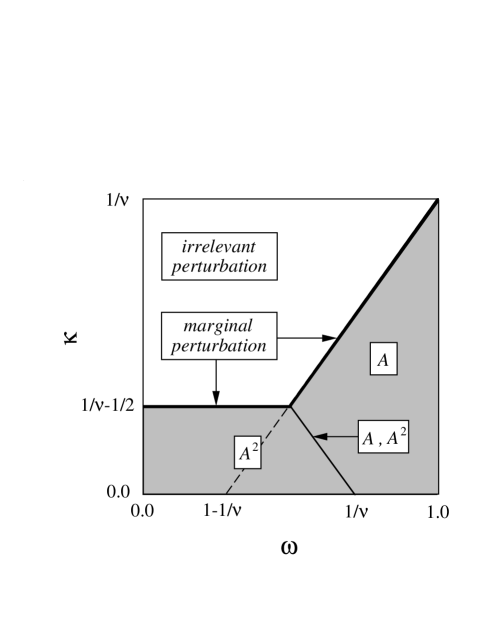
Figure 13: Relevance-irrelevance of aperiodic extended surface perturbations in a system with bulk correlation length exponent $\nu$. The perturbation is relevant in the shaded region. The order of the dominant perturbation terms is indicated, assuming that off-diagonal terms do not contribute.

We first consider off-diagonal contributions to $F^{(2)}$ which come from pairs of sites belonging to different layers. The corresponding amplitude $(A^{2})_{\rm od}$ scales as the product of two first-order amplitudes with:

$$({A^{\prime}}^{2})_{\rm od}=b^{2(-\kappa+\omega-1+1/\nu)}(A^{2})_{\rm od}\,.$$ (5.3)

One may notice that such cross-terms do not enter into the calculation of the surface magnetization of the $2d$ Ising model.

The diagonal contributions to $F^{(2)}$ involve pairs of sites belonging to the same layer and read:

$$-\beta F^{(2)}_{\rm d}=\frac{L^{d-1}}{2}\sum_{l}\sum_{\vec{r}_{\parallel}}\frac{A^{2}}{l^{2\kappa}}\,{\cal G}_{\varepsilon\varepsilon}(r_{\parallel})\,,$$ (5.4)

where $L^{d-1}$ is the surface of the layers. The density under the sums has dimension $2d-1$ whereas the correlation function has dimension $2x_{\rm e}$, where $x_{\rm e}$ is the scaling dimension of the bulk energy density, thus one obtains:

$$\frac{({A^{\prime}}^{2})_{\rm d}}{{l^{\prime}}^{2\kappa}}=b^{2d-1-2x_{\rm e}}\frac{(A^{2})_{\rm d}}{l^{2\kappa}}=b^{-1+2/\nu}\frac{(A^{2})_{\rm d}}{l^{2\kappa}}$$ (5.5)

and the diagonal second-order amplitude transforms as:

$$({A^{\prime}}^{2})_{\rm d}=b^{-1-2\kappa+2/\nu}(A^{2})_{\rm d}\,.$$ (5.6)

It is a relevant (irrelevant) variable when $\kappa\!<\!(>)-1/2+1/\nu$ and a marginal one when $\kappa\!=\!-1/2+1/\nu$.

The scaling dimension $y_{(A^{2})_{\rm d}}$ of $(A^{2})_{\rm d}$ has to be compared to the dimension $y_{A}$ of $A$ given in $(\ref{scala1})$ to see which term governs the critical behaviour when both are relevant. When $y_{(A^{2})_{\rm d}}\!>\!y_{A}$, i.e., when $\kappa\!<\!-\omega+1/\nu$, the second-order term dominates and one expects an $A^{2}$-dependence of the amplitudes in the stretched exponentials. On the line $\kappa\!=\!-\omega+1/\nu$ when $\kappa\!\leq\!-1/2+1/\nu$, linear and quadratic terms contribute together.

A summary of the relevance-irrelevance in the $(\kappa,\omega)$-plane is given in Fig. 13. It is in agreement with our findings of Sections 3 and 4 for the surface magnetization of the $2d$ Ising model. The order of the dominant contributions could be modified by the discarded off-diagonal second- or higher-order terms. As mentioned earlier for the $2d$ Ising model, there is a shift of the bulk critical coupling for the homogeneous aperiodic system on the line $\kappa\!=\!0$. Along this line the perturbation is irrelevant below $\omega\!=\!1-1/\nu$.

One may notice that the model shows some kind of universal behaviour. Both the amplitude $C(a)$ in the stretched exponential and the surface magnetic exponent $\beta_{\rm s}(a)$ are independent of the aperiodic sequence, provided the value of $\omega$ is such that the system belongs to the region $\kappa\leq 1/2$, $\kappa\!<\!1-\omega$ of Fig. 1 where the quadratic contribution dominates.

Let us now briefly discuss the behaviour of the first gap and the surface energy.

On a finite critical Ising chain, the first gap is known to scale as igloi97

$$\epsilon_{1}(L)\sim m_{\rm s,c}(L)\,P_{L}^{-1}\,\overline{m}_{\rm s,c}(L)\,,$$ (5.7)

where $\overline{m}_{\rm s,c}$ is the critical magnetization on the second surface and $P_{L}$ is the product of the couplings defined in Eq. (3.8). When $\kappa\!>\!0$ the bulk is unperturbed and, asymptotically, the second surface displays an ordinary surface transition. Thus the scaling dimension of $\overline{m}_{\rm s}$ is $\overline{x}{}_{\rm m}^{\rm s}\!=\!1/2$.

For relevant perturbations, with the notations of Appendix B, we have:

$$P_{L}^{-1}\simeq\exp(\frac{1}{2}B\,L^{\tau})\;.$$ (5.8)

When the surface transition is continuous $m_{\rm s,c}(L)$, given in Eq. (B.4), behaves as $P_{L}$. It follows that the first gap vanishes as a power of $L$. One expects in this case the unperturbed behaviour $\epsilon_{1}(L)\!\sim\!L^{-1}$ .

When the surface transition is first-order, the leading term in $m_{\rm s,c}(L)$ is a constant and there is no more compensation. The first gap is anomalous, it vanishes with an essential singularity. This behaviour is linked to the localization of the corresponding eigenvector $\boldsymbol{\phi}_{1}$, which itself is reponsible for the finite weight on the first component $\phi_{1}(1)$, leading to a non-vanishing surface magnetization peschel84 .

The scaling dimension $x_{\rm e}^{\rm s}$ of the surface energy can be deduced from the finite-size behaviour $e_{\rm s}\!=\!\langle 0|\sigma_{1}^{x}|\varepsilon\rangle$ where the state $|\varepsilon\rangle\!=\!\eta_{1}^{\dagger}\eta_{2}^{\dagger}|0\rangle$ is the lowest two-particle excitated state. This matrix element can be written as karevski95 :

$$e_{\rm s}=(\epsilon_{2}-\epsilon_{1})\phi_{1}(1)\phi_{2}(1)\,.$$ (5.9)

For relevant perturbations one expects an essential singularity since at least $\phi_{2}(1)$ should behave in this way.

In the case of a marginal perturbation, with the notations of Appendix B, one may write:

$$P_{L}^{-1}\simeq L^{B/2}=L^{-1/2+\beta_{\rm s}(a)}\,,$$ (5.10)

where $\beta_{\rm s}(a)$ is the surface magnetic exponent $\beta_{\rm s}$ when the transition is second-order or its continuation to negative values when the transition is first-order, i.e., when $\beta_{\rm s}\!=\!0$.

When the transition is second-order Eqs. (5.7) and (5.10) lead to:

$$\epsilon_{1}(L)\sim L^{-\beta_{\rm s}}\,L^{-1/2+\beta_{\rm s}}\,L^{-1/2}\sim L^{-1}\,,$$ (5.11)

i.e., to the unperturbed behaviour as above for relevant perturbations when the transition is continuous.

For the surface energy, Eq. (5.9) leads to the scaling dimension

$$x_{\rm e}^{\rm s}=1+2\beta_{\rm s}$$ (5.12)

if one assumes that $\phi_{2}(1)$ scale as $L^{-\beta_{\rm s}}$ too. This is known to be true either for the marginal HvL model berche90 or for the aperiodic version of the same model karevski95 where the couplings are modulated according to the Fredholm sequence dekking83 .

When the transition is first-order, due to the localization of $\boldsymbol{\phi}_{1}$, the scaling of the first excitation is anomalous gap :

$$\epsilon_{1}(L)\sim L^{-1+\beta_{\rm s}(a)}\,.$$ (5.13)

It decays faster than higher excitations since $\beta_{\rm s}(a)\!<\!0$.

For the surface energy, we conjecture the following behaviour:

$$x_{\rm e}^{\rm s}=1+\frac{\beta^{\prime}_{\rm s}}{2}=1-\beta_{\rm s}(a)\,.$$ (5.14)

The factor containing the excitations in Eq. (5.9) is dominated by $\epsilon_{2}$ which vanishes as $L^{-1}$. Furthermore we assumed that, like in Refs. karevski95 ; berche90 , $\phi_{2}(1)$ scales as $L^{-\beta^{\prime}_{\rm s}/2}$.

As for the HvL model, in the regime of first-order transition, the anomalous scaling of the first gap leads to an exponent asymmetry blote83 . For example, in the disordered phase, the exponent of the correlation length $\xi_{\parallel}$, along the surface of the semi-infinite system, is governed by the first gap and $\nu_{\parallel}\!=\!1-\beta_{\rm s}(a)$. In the ordered phase the first excitation vanishes and $\xi_{\parallel}\!\sim\epsilon_{2}^{-1}$ so that $\nu^{\prime}_{\parallel}\!=\!1$, like in the unperturbed system.

To conclude, let us mention that the case of random surface extended perturbations, which has fluctuation properties similar to the aperiodic case with $\omega\!=\!1/2$ igloi98 , is currently under study.

Appendix A: Log-periodic functions

The log-periodic function $c(l)$ defined in Eq. (3.10) is such that $c(b^{n}l)\!=\!c(l)$ where $b$ is the discrete dilatation factor of the aperiodic sequence. It can be generally written as a Fourier expansion,

$$c(l) = c_{0}+\sum_{k=1}^{\infty}c_{k}\,\cos[\theta_{k}(l)]\,,$$

$$\theta_{k}(l) = 2\pi k\,\frac{\ln l}{\ln b}+\varphi_{k}\,,$$ (A.1)

so that, in (3.12):

$$c_{\kappa}(j)=c_{0}+\sum_{k=1}^{\infty}c_{k}\frac{\sum_{l=1}^{j}l^{\omega-\kappa-1}\cos\theta_{k}(l)}{\sum_{l=1}^{j}l^{\omega-\kappa-1}}\,.$$ (A.2)

We are interested in the behaviour of $c_{\kappa}(j)$ at large $j$.

$\bullet$ When $\kappa\!<\!\omega$, let us write:

$$c_{\kappa}(j)=c_{0}+\sum_{k=1}^{\infty}c_{k}\Re[I_{k}(j)]\,,$$ (A.3)

where:

$$I_{k}(j) = {\rm e}^{{\rm i}\varphi_{k}}\frac{\sum_{l=1}^{j}l^{\omega-\kappa-1+{\rm i}2\pi k/\ln b}}{\sum_{l=1}^{j}l^{\omega-\kappa-1}}$$ (A.4)

$$\simeq {\rm e}^{{\rm i}\varphi_{k}}\frac{\int_{0}^{j}{\rm d}l\,l^{\omega-\kappa-1+{\rm i}2\pi k/\ln b}}{\int_{0}^{j}{\rm d}l\,l^{\omega-\kappa-1}}\,,$$

so that:

$$\Re[I_{k}(j)] \simeq \frac{\cos[\theta_{k}(j)]+\alpha_{k}\,\sin[\theta_{k}(j)]}{1+\alpha_{k}^{2}}\,,$$

$$\alpha_{k} = \frac{2\pi k}{(\omega-\kappa)\ln b}\,.$$ (A.5)

It follows that $c_{\kappa}(j)$ oscillates log-periodically around $c_{0}$. The Fourier coefficients $c_{k}$ are divided by $k$ when $k$ is large or when $\kappa$ is close to $\omega$. The effective constant $\overline{c}$ in (3.13) can be taken as the value of $c_{\kappa}(j)$ which gives the main contribution to the function in which it enters.

$\bullet$ When $\kappa\!=\!\omega$, replacing the sums over $l$ in (A.2) by integrals, the change of variable $u\!=\!\ln l$ leads to:

$$c_{\kappa}(j)\simeq c_{0}+\sum_{k=1}^{\infty}\frac{c_{k}}{\ln j}\int_{0}^{\ln j}{\rm d}u\,\cos\left(2\pi k\frac{u}{\ln b}+\varphi_{k}\right)\,.$$ (A.6)

Thus $\lim_{j\to\infty}c_{\kappa}(j)\!=\!c_{0}$ and $\overline{c}$ is the constant term in the Fourier expansion of $c(l)$.

$\bullet$ When $\kappa\!>\!\omega$, according to (A.4), the asymptotic expression of $c_{\kappa}(j)$ can be written in terms of $\zeta$ functions with:

$$I_{k}(\infty)={\rm e}^{{\rm i}\varphi_{k}}\frac{\zeta(1+\kappa-\omega-{\rm i}2\pi k/\ln b)}{\zeta(1+\kappa-\omega)}\,.$$ (A.7)

Thus, in this case too, $c_{\kappa}(j)$ tends to a well-defined limiting value giving $\overline{c}$.

Appendix B: Amplitudes and exponents

We study successively the temperature-dependence of the surface magnetization near the critical point as well as its size-dependence at criticality.

We first consider the case of relevant perturbations where the leading contribution to $\ln P_{j}$ is some positive power of $j$. The sum $S\!=\!m_{\rm s}^{-2}$ in Eq. (3.8) can be then replaced by an integral of the form peschel84 ; igloi94

$$S(t)\simeq\int_{0}^{\infty}{\rm d}j\,\lambda^{-2j}P_{j}^{-2}\simeq\int_{0}^{\infty}{\rm d}j\,\exp(-tj+Bj^{\tau})\,,$$ (B.1)

where we used the definition of $t$ given in (3.4). For the finite-size behaviour at the critical point, $t\!=\!0$, the sum is cut off at L so that:

$$S_{\rm c}(L)\simeq\int_{0}^{L}{\rm d}j\,P_{j}^{-2}\simeq\int_{0}^{L}{\rm d}j\,\exp(Bj^{\tau})\,,$$ (B.2)

When $B\!>\!0$, the integral can be evaluated using Laplace’s method when $0\!<\!\tau\!<\!1$ and, up to a power law prefactor, one obtains:

$$m_{\rm s}(t)\sim\exp\left[-\frac{1-\tau}{2\tau}(\tau B)^{1/(1-\tau)}\,t^{-\tau/(1-\tau)}\right]\,.$$ (B.3)

The main contribution to $S_{\rm c}(L)$ comes from the vicinity of the upper limit. Expanding the argument of the exponential around $L$ leads to:

$$m_{\rm s,c}(L)\sim\exp\left[-\frac{1}{2}B\,L^{\tau}\right]\,.$$ (B.4)

When $B\!<\!0$, expanding $\exp(-tj)$ in (B.1) and integrating term by term gives:

$$m_{\rm s}(t)\simeq\left[\frac{\tau|B|^{1/\tau}}{\Gamma(1/\tau)}\right]^{1/2}\left[1+\frac{\Gamma(2/\tau)}{2\Gamma(1/\tau)|B|^{1/\tau}}\,t+\cdots\right]\,.$$ (B.5)

Let us now look for the values of $B$ and $\tau$ when $\kappa$ varies.

$\bullet$ When $1-\omega\!<\!\kappa\!<\!\omega$, the term which is linear in $a$ dominates in (3.13), so that:

$$P_{j}^{-2}\simeq\exp\left[\frac{4\overline{c}a}{\omega-\kappa}j^{\omega-\kappa}\right]\,,$$ (B.6)

which leads to the expressions given in Eqs. (3.14) and (3.15).

$\bullet$ When $1-\omega\!=\!\kappa\!<\!\omega$, both terms in (3.13) are of the same order and

$$P_{j}^{-2}\simeq\exp\left[\frac{4\overline{c}a+a^{2}}{1-2\kappa}j^{1-2\kappa}\right]\,,$$ (B.7)

leading to (3.16) and (3.17).

$\bullet$ When $\kappa\!<\!{\rm min}(1-\omega,1/2)$, the term in $a^{2}$ governs the behaviour of (3.13), so that

$$P_{j}^{-2}\simeq\exp\left[\frac{a^{2}}{1-2\kappa}j^{1-2\kappa}\right]\,,$$ (B.8)

from which Eqs. (3.18) and (3.19) follow.

Next we consider the case of marginal perturbations where $P_{j}$ behaves as $j^{-B/2}$. When $B\!>\!-1$, $S$ in Eq. (3.8) can be rewritten as peschel84

$$S(t)\simeq\int_{0}^{\infty}{\rm d}j\,\lambda^{-2j}P_{j}^{-2}\simeq\int_{0}^{\infty}{\rm d}j\,j^{B}{\rm e}^{-tj}\,,$$ (B.9)

or, at the critical point,

$$S_{\rm c}(L)\simeq\int_{0}^{L}{\rm d}j\,P_{j}^{-2}\simeq\int_{0}^{L}{\rm d}j\,j^{B}\,.$$ (B.10)

For the $t$-dependence, one obtains:

$$m_{\rm s}(t) \simeq \left[t^{-1-B}\int_{0}^{\infty}{\rm d}u\,u^{B}{\rm e}^{-u}\right]^{-1/2}$$ (B.11)

$$= [\Gamma(B+1)]^{-1/2}\,t^{(1+B)/2}\,,$$

whereas:

$$m_{\rm s,c}(L)\simeq(1+B)^{1/2}L^{-(1+B)/2}$$ (B.12)

When $B\!<\!-1$, the integrals in (B.9) and (B.10) diverge at their lower limits. The main contribution, coming from small values of $j$, must be treated more carefully. For this purpose let us split $S$ into two parts as:

$$S(t)=1+\sum_{j=1}^{\infty}j^{-|B|}+\sum_{j=1}^{\infty}({\rm e}^{-tj}-1)j^{-|B|}\,.$$ (B.13)

The first sum gives $\zeta(|B|)$ whereas the second sum can be transformed using the Euler-MacLaurin summation formula:

$$\sum_{j=1}^{\infty}f(j,t)=\int_{1}^{t^{-1}}\!\!{\rm d}j\,f(j,t)+\int_{t^{-1}}^{\infty}\!\!{\rm d}j\,f(j,t)+O(t)\,.$$ (B.14)

The change of variable $u\!=\!tj$ leads to:

$$S(t) = m_{\rm s,c}^{-2}+t^{|B|-1}\Big{[}\int_{t}^{1}\!\!{\rm d}u\,({\rm e}^{-u}-1)u^{-|B|}+$$ (B.15)

$$\qquad\qquad+\int_{1}^{\infty}\!\!{\rm d}u\,({\rm e}^{-u}-1)u^{-|B|}\Big{]}\,,$$

where $m_{\rm s,c}\!=\![1+\zeta(|B|)]^{-1/2}$. The $t$-dependence of the first integral is obtained through an expansion of the exponential and the second is a constant. Collecting the different terms gives

$$S(t)=m_{\rm s,c}^{-2}+{\rm const}\,t^{|B|-1}+O(t)$$ (B.16)

and

$$m_{\rm s}(t)=m_{\rm s,c}+{\rm const}\,t^{|B|-1}+O(t)\,.$$ (B.17)

For the size-dependence at criticality, one may write:

$$S_{\rm c}(L) = 1+\sum_{j=1}^{L}j^{-|B|}$$ (B.18)

$$= 1+\sum_{j=1}^{\infty}j^{-|B|}-\int_{L}^{\infty}{\rm d}j\,j^{-|B|}+O(L^{-|B|})$$

$$= m_{\rm s,c}^{-2}+\frac{L^{1-|B|}}{1-|B|}+O(L^{-|B|})\,,$$

so that:

$$m_{\rm s,c}(L)=m_{\rm s,c}+\frac{m_{\rm s,c}^{3}}{2(|B|-1)}\,L^{-|B|+1}\,.$$ (B.19)

Finally, we identify the expression of the exponent $B$ for $\kappa$-values where a marginal behaviour is obtained.

$\bullet$ When $\kappa\!=\!\omega\!>\!1/2$, the linear term in (3.13) is the dominant one and yields:

$$P_{j}^{-2}\simeq j^{4\overline{c}a}\,,$$ (B.20)

from which the exponents in (3.20) and (3.21) follow.

$\bullet$ When $\kappa\!=\!\omega\!=\!1/2$, the linear and quadratic terms in Eq. (3.13) contribute, so that

$$P_{j}^{-2}\simeq j^{4\overline{c}a+a^{2}}\,,$$ (B.21)

leading to (3.22) and (3.23).

$\bullet$ When $\kappa\!=\!1/2$ and $\omega\!<\!1/2$, the leading contribution in (3.13) is the quadratic one,

$$P_{j}^{-2}\simeq j^{a^{2}}\,,$$ (B.22)

which gives the exponent in Eq. (3.24).

References

- (1) T. W. Burkhardt, J. Cardy, J. Phys. A 20, L233 (1987); T. W. Burkhardt, H. W. Diehl, Phys. Rev. B 50, 3894 (1994). This scaling relation is true at the ordinary and extraordinary transitions but at the special transition, see E. Eisenriegler, M. Krech, S. Dietrich, Phys. B 53, 14 377 (1996) and references therein.
- (2) K. Binder, Phase Transitions and Critical Phenomena, Vol. 8, edited by C. Domb and J. L. Lebowitz (Academic Press, London, 1983), p. 20.
- (3) H. J. Hilhorst, J. M. J. van Leeuwen, Phys. Rev. Lett. 47, 1188 (1981).
- (4) R. Cordery, Phys. Rev. Lett. 48, 215 (1982); T. W. Burkhardt, Phys. Rev. Lett. 48, 216 (1982); T. W. Burkhardt, Phys. Rev. B 25, 7048 (1982).
- (5) H. W. J. Blöte, H. J. Hilhorst, Phys. Rev. Lett. 51, 20 (1983); H. W. J. Blöte, H. J. Hilhorst, J. Phys. A 18, 3039 (1985).
- (6) T. W. Burkhardt, I. Guim, Phys. Rev. B 29, 508 (1984); T. W. Burkhardt, I. Guim, H. J. Hilhorst, J. M. J. van Leeuwen, Phys. Rev. B 30, 1486 (1984); T. W. Burkhardt, F. Iglói, J. Phys. A 23, L633 (1990); R. Z. Bariev, L. Turban, Phys. Rev. B 45, 10 761 (1992); F. Iglói, L. Turban, Phys. Rev. B 47, 3404 (1993); L. Turban, B. Berche, J. Phys. A 26, 3131 (1993).
- (7) J. M. Luck, J. Stat. Phys. 72, 417 (1993); J. M. Luck, Europhys. Lett. 24, 359 (1993); F. Iglói, J. Phys. A 26, L703 (1993).
- (8) M. Queffélec, Substitutional Dynamical Systems, Lecture Notes in Mathematics, Vol. 1294, edited by A. Dold and B. Eckmann (Springer, Berlin, 1987).
- (9) J. Kogut, Rev. Mod. Phys. 51, 659 (1979).
- (10) P. Pfeuty, Ann. Phys. (Paris) 57, 79 (1970).
- (11) P. Jordan, E. Wigner, Z. Phys. 47, 631 (1928).
- (12) E. H. Lieb, T. D. Schultz, D. C. Mattis, Ann. Phys. (N.Y.) 16, 406 (1961).
- (13) I. Peschel, Phys. Rev. B 30, 6783 (1984).
- (14) L. Turban, F. Iglói, B. Berche, Phys. Rev. B 49, 12 695 (1994); B. Berche, P. E. Berche, M. Henkel, F. Iglói, P. Lajkó, S. Morgan, L. Turban, J. Phys. A 28, L165 (1995); P. E. Berche, B. Berche, L. Turban, J. Phys. I France 6, 621 (1996); F. Iglói, L. Turban, Phys. Rev. Lett. 77, 1206 (1996); J. Hermisson, U. Grimm, M. Baake, J. Phys. A 30, 7315 (1997).
- (15) F. Iglói, L. Turban, D. Karevski, F. Szalma, Phys. Rev. B 56, 11 031 (1997); J. Hermisson, U. Grimm, Phys. Rev. B 57, 673 (1998).
- (16) The critical coupling of the inhomogeneous Ising quantum chain is such that . See P. Pfeuty, Phys. Lett. 72A, 245 (1979).
- (17) M. Dekking, M. Mendès-France, A. van der Poorten, Math. Intelligencer 4, 130 (1983).
- (18) M. Henkel, G. Schütz, J. Phys. A 21, 2617 (1988).
- (19) D. Karevski, G. Palágyi, L. Turban, J. Phys. A 28,45 (1995).
- (20) B. Berche, L. Turban, J. Phys. A 23, 3029 (1990).
- (21) One may notice that for a symmetric system, where both surfaces are perturbed, the first gap scales as . See for example Ref. karevski95 .
- (22) F. Iglói, D. Karevski, H. Rieger, Eur. Phys. J. B 5, 613 (1998).
- (23) F. Iglói, L. Turban, Europhys. Lett. 39, 91 (1994).