-1cm 0cm 0.3cm

Vortex Stabilization in Dilute Bose-Einstein Condensate Under Rotation

1 Introduction

There has been much attention focused on the Bose-Einstein condensation (BEC) experimentally and theoretically since it was realized in dilute alkali atom gases in 1995 .${}^{\hbox{\immediate{\bf{?}},\penalty 1000\hskip 0.91003pt plus 0.70004pt minus 0.70004pt{\bf{?}},\penalty 1000\hskip 0.91003pt plus 0.70004pt minus 0.70004pt{\bf{?}})}}$ The condensates have atom number typically $\sim O(10^{6})$ for ²³Na and ⁸⁷Rb, their BEC transition temperatures are in a range of $O(\mu{\rm K})$, and they are usually confined magnetically in a harmonic trap .${}^{\hbox{\immediate{\bf{?}},\penalty 1000\hskip 0.91003pt plus 0.70004pt minus 0.70004pt{\bf{?}},\penalty 1000\hskip 0.91003pt plus 0.70004pt minus 0.70004pt{\bf{?}})}}$

In these systems, it is natural to expect a quantized vortex which has been already much studied in a superconductor (Fermion) and ⁴He (Boson) for a long time. ${}^{\hbox{\immediate{\bf{?}},\penalty 1000\hskip 0.91003pt plus 0.70004pt minus 0.70004pt{\bf{?}})}}$ While various microscopic theories for a vortex in Fermionic systems such as BCS-Gor’kov or Bogoliubov-de Gennes theories are developed, ${}^{\hbox{\immediate{?})}}$ the corresponding mean-field framework for a vortex in Bosonic systems originally due to Bogoliubov has not fully examined yet. ${}^{\hbox{\immediate{\bf{?}},\penalty 1000\hskip 0.91003pt plus 0.70004pt minus 0.70004pt{\bf{?}},\penalty 1000\hskip 0.91003pt plus 0.70004pt minus 0.70004pt{\bf{?}})}}$ Therefore, it is urgent to examine whether or not the widely used Bogoliubov theory, which has been quite successful so far for describing present BEC systems without a vortex, ${}^{\hbox{\immediate{?})}}$ can also yield a stable vortex.

In connection with the present dilute BEC systems of alkali atom gases, theoretical ${}^{\hbox{\immediate{\bf{?}},\penalty 1000\hskip 0.91003pt plus 0.70004pt minus 0.70004pt{\bf{?}},\penalty 1000\hskip 0.91003pt plus 0.70004pt minus 0.70004pt{\bf{?}},\penalty 1000\hskip 0.91003pt plus 0.70004pt minus 0.70004pt{\bf{?}},\penalty 1000\hskip 0.91003pt plus 0.70004pt minus 0.70004pt{\bf{?}},\penalty 1000\hskip 0.91003pt plus 0.70004pt minus 0.70004pt{\bf{?}},\penalty 1000\hskip 0.91003pt plus 0.70004pt minus 0.70004pt{\bf{?}},\penalty 1000\hskip 0.91003pt plus 0.70004pt minus 0.70004pt{\bf{?}})}}$ and experimental studies on a vortex have just started. So far there is no report to observe a vortex experimentally. One possible reason of the difficulty in producing a vortex is that gases are confined magnetically in a harmonic trap and this object is not so easy to manipulate it under rotation as compared with superfluid ⁴He in a bucket. There are some theoretical proposals ${}^{\hbox{\immediate{?},\penalty 1000\hskip 0.91003pt plus 0.70004pt minus 0.70004pt{?})}}$ to realize the vortex state in this situation. The persistent rotation may be realized by shining moving laser on a large BEC system, which is examined theoretically by Marzlin et al. .${}^{\hbox{\immediate{?})}}$

Previously, we examined the stability problem of a vortex in BEC systems confined by a rigid wall ${}^{\hbox{\immediate{\bf{?}})}}$ and by a harmonic potential ${}^{\hbox{\immediate{\bf{?}})}}$ within the framework of Hartree-Fock Bogoliubov theory both at $T$=0 and $T\neq 0$. The conclusions we have reached are summarized as follows: (1) At $T$=0 the vortex is unstable in the non-selfconsistent Bogoliubov theory and the self-consistent Popov theory. ${}^{\hbox{\immediate{?},\penalty 1000\hskip 0.91003pt plus 0.70004pt minus 0.70004pt{?})}}$ (2) Above a certain temperature the vortex becomes stabilized by the presence of the increased non-condensate fraction localized at the vortex center, which effectively acts as a pinning potential, preventing it from spiraling out. ${}^{\hbox{\immediate{?})}}$ (3) Even at $T=0$, the external laser-induced potential at the vortex center has a similar effect to stabilize the vortex. ${}^{\hbox{\immediate{?})}}$ In these discussions, the stability of the vortex state is examined by the positive sign of the lowest eigenvalue ${}^{\hbox{\immediate{?})}}$ while its negative sign means the eigenvalue becomes lower than the ground state energy. We call this stability “local stability”. The question of this type is still under lively discussions. ${}^{\hbox{\immediate{?},\penalty 1000\hskip 0.91003pt plus 0.70004pt minus 0.70004pt{?},\penalty 1000\hskip 0.91003pt plus 0.70004pt minus 0.70004pt{?},\penalty 1000\hskip 0.91003pt plus 0.70004pt minus 0.70004pt{?},\penalty 1000\hskip 0.91003pt plus 0.70004pt minus 0.70004pt{?},\penalty 1000\hskip 0.91003pt plus 0.70004pt minus 0.70004pt{\bf{?}})}}$

As in ⁴He system under persistent rotation around a symmetry axis, ${}^{\hbox{\immediate{?})}}$ another stability criterion of the vortex state is to compare the total energy of the vortex system with that of the non-vortex system. We call this stability “global stability”, considering the energy landscape of the configurational space. Here we study these two types of the vortex stability problem simultaneously, when the BEC system is kept in rotation at $T=0$.

It is expected that above a certain critical angular velocity $\Omega_{\rm global}$, a vortex nucleates as in superfluid ⁴He system or as in the lower critical field $H_{c1}$ in a type II superconductor. As we will see in detail, the applied rotation tends to stabilize a vortex in general, therefore the above local stability criterion of the vortex formation is also satisfied even at $T=0$, which is characterized by another angular velocity $\Omega_{\rm local}$. The purposes of this paper are to determine these characteristic angular velocities; $\Omega_{\rm local}$ and $\Omega_{\rm global}$ and to examine the relationship between them. Because the previous study ${}^{\hbox{\immediate{?},\penalty 1000\hskip 0.91003pt plus 0.70004pt minus 0.70004pt{?})}}$ corresponds to $\Omega=0$ here, we will gain further understanding even for the local stability problem through this study for various $\Omega$’s.

To attack this problem, we solve the eigenvalue equation of the Bogoliubov theory, which is non-selfconsistent. If it gives a negative eigenvalue under a given condensate spatial profile determined by the associated no-linear Schrödinger type equation (Gross-Pitaevskii equation, or GP), the quantized vortex cannot be stable even for a self-consistent calculation.

The arrangement of the paper is as follows: After giving a brief description of the Bogoliubov theory in §2, the vortex stability problem in a system trapped harmonically is discussed in §3. The numerical procedure for solving the GP equation and the eigenvalue equation is the same as before, described in refs. ? and ?. The final section is devoted to discussions and summary.

2 Formulation of Bogoliubov Equation Under Rotation

2.1 General formulation

We start with a system of interacting Bosons. Two particles at ${\bf r}$ and ${\bf r}^{\prime}$ interact with the potential $g\delta({\bf r}-{\bf r}^{\prime})$ where $g$ is a positive (repulsive) constant proportional to the s-wave scattering length $a$, namely $g=4\pi\hbar^{2}a/m$ ($m$ the particle mass). The system is kept under rotation with the angular velocity $\omega$ by an external force. The relevant hamiltonian $\hat{\rm H}_{\rm rot}$ with the extra rotation term can be written as:

$$\hat{\rm H}_{\rm rot}=\hat{\rm H}-{\bf\omega}\cdot\int{\bf r}\times{\bf p}({\bf r}){\rm d}{\bf r}$$ (1)

where

$$\hat{\rm H} = \int{\rm d}{\bf r}\hat{\Psi}^{\dagger}({\bf r})\left\{-\frac{\hbar^{2}\nabla^{2}}{2m}+V({\bf r})-\mu\right\}\hat{\Psi}({\bf r})$$ (2)

$$+\frac{g}{2}\!\!\int\!\!{\rm d}{\bf r}\hat{\Psi}^{\dagger}({\bf r})\hat{\Psi}^{\dagger}({\bf r})\hat{\Psi}({\bf r})\hat{\Psi}({\bf r}),$$

${\bf p}(\bf r)$ is the momentum operator, $\mu$ is the chemical potential, and $V({\bf r})$ is the confining potential.

Following the standard method, we decompose the field operator $\hat{\Psi}$ as

$$\hat{\Psi}({\bf r}) = \hat{\psi}({\bf r})+\phi({\bf r})$$ (3)

$$\phi({\bf r}) \equiv \langle\hat{\Psi}({\bf r})\rangle.$$ (4)

We substitute the above decomposition eq. (3) into eq. (1) and ignore the higher order terms such as $\hat{\psi}^{\dagger}\hat{\psi}\hat{\psi}$, $\hat{\psi}^{\dagger}\hat{\psi}^{\dagger}\hat{\psi}$, and $\hat{\psi}^{\dagger}\hat{\psi}^{\dagger}\hat{\psi}\hat{\psi}$ terms. Then we rewrite the operator $\hat{\psi}({\bf r})$ as

$$\hat{\psi}({\bf r})=\sum_{q}\left[u_{q}({\bf r})\eta_{q}-v_{q}^{*}({\bf r})\eta_{q}^{\dagger}\right]$$ (5)

where $\eta_{q}$ ($\eta_{q}^{\dagger}$) is the annihilation (creation) operator and $u_{q}({\bf r})$ and $v_{q}({\bf r})$ are the wave functions, and the subscript $q$ denotes the quantum number.

2.2 Cylindrical system

We consider a cylindrically symmetric system and a vortex line, if exists, passes through the center of a cylinder, coinciding with the rotation axis. We use the cylindrical coordinates: ${\bf r}=(r,\theta,z)$. The system is trapped radially by a harmonic potential

$$V(r)=\frac{1}{2}m(2\pi\nu)^{2}r^{2},$$ (6)

and is periodic along the $z$-axis whose length is $L$. We focus on the lowest eigenstates of the momentum along $z$-axis and the quantum number ${\bf q}$ in eq. (5) is written as $(q_{r},q_{\theta})$, where $q_{r}=1,2,3,\cdots$ and $q_{\theta}=0,\pm 1,\pm 2,\cdots$.

The condensate wave function $\phi({\bf r})$ is expressed as

$$\phi(r,\theta,z)=\phi(r){\rm e}^{{\rm i}w\theta}$$ (7)

where $\phi(r)$ is a real function and $w$ is the winding number. The case $w=0$ corresponds to a system without a vortex and $w=1(w=2)$ corresponds to a system with a singly (doubly) quantized vortex. The $w>2$ case is not considered in this paper. The phases of $u_{q}({\bf r})$ and $v_{q}({\bf r})$ can be written as

$$u_{q}({\bf r}) = u_{q}(r){\rm e}^{{\rm i}(q_{\theta}+w)\theta}$$ (8)

$$v_{q}({\bf r}) = v_{q}(r){\rm e}^{{\rm i}(q_{\theta}-w)\theta}.$$ (9)

The condition that the first order term in $\hat{\psi}({\bf r})$ of our hamiltonian vanish is

$$\Bigl{[}-\frac{\hbar^{2}}{2m}\left\{\frac{{{\rm d}}^{2}}{{{\rm d}}r^{2}}+\frac{1}{r}\frac{{\rm d}}{{{\rm d}}r}-\frac{w^{2}}{r^{2}}\right\}-\mu$$

$$+V(r)+g\phi^{2}(r)+\hbar\omega w\Bigr{]}\phi(r) = 0.$$ (10)

This non-linear Schrödinger type equation is called the Gross-Pitaevskii equation. The condition that the hamiltonian be diagonalized gives the coupled eigenvalue equations for $u_{q}({\bf r})$, and $v_{q}({\bf r})$ whose eigenvalue is $\varepsilon_{q}$:

$$\Bigl{[}-\frac{\hbar^{2}}{2m}\left\{\frac{{\rm d}^{2}}{{\rm d}r^{2}}+\frac{1}{r}\frac{{\rm d}}{{\rm d}r}-\frac{(w+q_{\theta})^{2}}{r^{2}}\right\}-\mu$$

$$+V(r)+2g\phi^{2}(r)+\hbar\omega(w+q_{\theta})\Bigr{]}u_{q}(r)$$

$$-g\phi^{2}(r)v_{q}(r) = \varepsilon_{q}u_{q}(r)$$ (11)

$$\Bigl{[}-\frac{\hbar^{2}}{2m}\left\{\frac{{\rm d}^{2}}{{\rm d}r^{2}}+\frac{1}{r}\frac{{\rm d}}{{\rm d}r}-\frac{(w-q_{\theta})^{2}}{r^{2}}\right\}-\mu$$

$$+V(r)+2g\phi^{2}(r)+\hbar\omega(w-q_{\theta})\Bigr{]}v_{q}(r)$$

$$-g\phi^{2}(r)u_{q}(r) = -\varepsilon_{q}v_{q}(r).$$ (12)

The normalization condition for $\phi({\bf r})$, $u_{q}({\bf r})$, and $v_{q}({\bf r})$ are

$$2\pi\int|\phi(r)|^{2}r{\rm d}r=\frac{N}{L},$$ (13)

$$2\pi\int\left\{u_{p}^{*}(r)u_{q}(r)-v_{p}^{*}(r)v_{q}(r)\right\}r{\rm d}r=\frac{1}{L}\delta_{p,q},$$ (14)

where $N$ is the total particle number.

The following symmetry relation should be noted:

$$(u,v,\varepsilon)\mbox{ at }q_{\theta}=n\Leftrightarrow(v,u,-\varepsilon)\mbox{ at }q_{\theta}=-n$$ (15)

We determine the signs of $q_{\theta}$ and $\varepsilon$ by the normalization condition eq. (14). The set of the eqs. (10), (11), (12), (13), and (14) constitute Bogoliubov theory of our system.

When this Bogoliubov theory is extended to a finite temperature such as Popov approximation (see for example ref. ?), the eigenstates characterized by the eigenfunctions $u_{q}$ and $v_{q}$, and the eigenvalue $\varepsilon_{q}$ are interpreted as the quasiparticles of the system which contribute to the total particle density as $f(\varepsilon)(|u_{q}|^{2}+|v_{q}|^{2})$ with $f(\varepsilon)$ being the Bose distribution function.

The energy of the system is given by

$$E = \langle\hat{H}_{\rm rot}\rangle+\mu N$$ (16)

$$= E_{\phi}+\sum_{q}(\mu-\varepsilon_{q})2\pi L\!\int|v_{q}(r)|^{2}r\,{\rm d}r.$$

$$E_{\phi} = 2\pi L\!\int\!\biggl{[}-\frac{\hbar^{2}}{2m}\phi^{*}(r)\!\biggl{(}\frac{{\rm d}^{2}}{{\rm d}r^{2}}+\frac{1}{r}\frac{{\rm d}}{{\rm d}r}-\frac{w^{2}}{r^{2}}\biggr{)}\!\phi(r)$$ (17)

$$+V(r)|\phi(r)|^{2}+\frac{g}{2}|\phi(r)|^{4}\biggr{]}r\,{\rm d}r-w\hbar\omega N.$$

Note that the coefficient of $\omega$ in eq. (17) is a constant. Although $\varepsilon$’s and $v$’s are affected by the angular velocity $\omega$, these contributions to $E$ are negligibly small and we will use $E_{\phi}$ as the total energy from now on.

2.3 Normalization

The condensate has $N$ particles in the length $L$ and the area density is $n_{z}=N/L$. The mass of a particle is $m$ and the s-wave scattering length is $a$. The length $r$ is measured as $r^{\prime}=(\sqrt{2mh\nu}/\hbar)r$. We introduce the density unit $n_{0}\equiv\sqrt{h\nu/g}$ where $g=4\pi\hbar^{2}a/m$. The density and energy are scaled by $n_{0}$ and $h\nu$ respectively. Therefore, the normalized quantities are: $\phi^{\prime}(r^{\prime})\equiv\frac{1}{\sqrt{n_{0}}}\phi(r)$, $u^{\prime}(r^{\prime})\equiv\frac{1}{\sqrt{n_{0}}}u(r)$, $v^{\prime}(r^{\prime})\equiv\frac{1}{\sqrt{n_{0}}}v(r)$, $\varepsilon^{\prime}_{q}\equiv\frac{1}{h\nu}\varepsilon_{q}$, and $\mu^{\prime}\equiv\frac{1}{h\nu}\mu$. The angular velocity $\omega$ is also scaled by $2\pi\nu$ and the normalized rotation is $\Omega\equiv\frac{\omega}{2\pi\nu}$.

Equation (10) with eq. (6) becomes in a dimensionless form

$$\Bigl{[}-\left\{\frac{{\rm d}^{2}}{{\rm d}r^{\prime 2}}+\frac{1}{r^{\prime}}\frac{{\rm d}}{{\rm d}r^{\prime}}-\frac{w^{2}}{r^{\prime 2}}\right\}-\mu^{\prime}$$

$$+\frac{1}{4}r^{\prime 2}+\phi^{\prime 2}(r^{\prime})+w\Omega\Bigr{]}\phi^{\prime}(r^{\prime}) = 0.$$ (18)

Equations (11) and (12) is transformed in a similar way. Equations (13) and (14) are rewritten as

$$\int|\phi^{\prime}(r)|^{2}r^{\prime}{\rm d}r^{\prime} = 4an_{z}.$$ (19)

$$\int\left\{u_{p}^{\prime*}(r^{\prime})u_{q}^{\prime}(r^{\prime})-v_{p}^{\prime*}(r^{\prime})v_{q}^{\prime}(r^{\prime})\right\}r^{\prime}{\rm d}r^{\prime} = \frac{4a}{L}\delta_{p,q}.$$ (20)

The energy $E_{\phi}$ is rewritten as

$$\frac{E_{\phi}}{h\nu N} = \frac{1}{4an_{z}}\int\biggl{[}\!-\phi^{*\prime}(r^{\prime})\!\biggl{(}\frac{{\rm d}^{2}}{{\rm d}r^{\prime 2}}+\frac{1}{r^{\prime}}\frac{{\rm d}}{{\rm d}r^{\prime}}-\frac{w^{2}}{r^{\prime 2}}\biggr{)}\!\phi^{\prime}(r^{\prime})$$ (21)

$$+\frac{1}{4}r^{\prime 2}|\phi^{\prime}(r^{\prime})|^{2}+|\phi^{\prime}(r^{\prime})|^{4}\biggr{]}r^{\prime}{\rm d}r^{\prime}-w\Omega.$$

Here $4an_{z}$ and $\frac{4a}{L}$ are just dimensionless numbers. Since the parameter $\frac{4a}{L}$ does not change the following results within the present Bogoliubov framework, the system is characterized by the number $an_{z}$ and the normalized rotation $\Omega=\frac{\omega}{2\pi\nu}$.

3 Two Kinds of Stability

We solve the coupled equations; eqs. (10), (11), (12), and (14) for the gas of ²³Na atoms trapped radially by a harmonic potential eq. (6). The area density per unit length along the $z$-axis is chosen to be $an_{z}=2.75\sim 137.5$. (When the scattering length is $a=2.75{\rm nm}$, the area density $n_{z}$ varies from $0.1$ to $5$ ($10^{4}/\mu{\rm m}$).) We use the normalized number $\Omega$ to indicate the angular velocity $\omega$. $\Omega$ varies from $0$ to $1$.

Since the GP equation eq. (10) is detached from the rest of the equations, it is easy to know the spatial profile of the condensate $\phi^{2}(r)$ by solving the GP equation. Figure 1 shows the typical density distribution of the system with and without the vortex along the radial direction. The doubly quantized vortex $w=2$ case is also plotted for comparison.

Fig.  1: The particle number density distribution $\phi^{2}(r)$ along the radial direction. Dashed (dotted) line is the singly (doubly) quantized vortex case $w=1$ ($w=2$) while solid line corresponds to the non-vortex case. To draw this figure in actual units, we use the following parameters: the scattering length $a=2.75{\rm nm}$, $m=3.81\times 10^{-26}{\rm kg}$, the radial trapping frequency $\nu=100{\rm Hz}$, and $n_{z}=2\times 10^{4}/\mu{\rm m}$.

3.1 Eigenvalues — local stability

When the lowest eigenvalue of the eigenvalue equations; eqs. (11) and (12) is negative in this formulation, the fundamental assumption of BEC is broken down as mentioned before. In this framework, the eigenstate with negative eigenvalue means that the system is unstable. Suppose that the negative eigenvalue appears in the vortex system while it dose not appear in the corresponding non-vortex system. Then the vortex state is unstable and prohibited against the non-vortex system. Dodd et al. ${}^{\hbox{\immediate{?})}}$ first consider the lowest eigenstate problem in the vortex state under $\Omega=0$, suggesting the presence of the negative eigenvalue for a harmonic potential.

We perform here the extensive computations for solving the eigenvalue equations to know the lowest eigenvalue under various external angular velocities $\Omega$. We show below the results of $an_{z}=55$ as an example. In Fig. 2, the lowest edge of the lowest eigenvalues, above which other eigenvalues are densely distributed, is plotted as a function of the quantum number $q_{\theta}$ for several $\Omega$’s. In the small $\Omega$ cases the lowest eigenvalue occurs for the eigenstate characterized by the quantum number $q_{\theta}=-1$, while in the larger $\Omega$ cases some positive eigenvalue of $q_{\theta}$ around $q_{\theta}\sim 10$ becomes negative as $\Omega$ increases. The eigenvalue at $q_{\theta}=0$ does not change with $\Omega$.

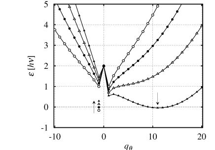
Fig.  2: The lowest edge of the eigenvalues along $q_{\theta}$ for selected angular velocities $\Omega$’s. Circles, filled circles, triangles, and filled triangles correspond to $\Omega$ = 0, 0.15, 0.3, and 0.45 respectively. The eigenvalues at $q_{\theta}=-1$ move up while the eigenvalues in $q_{\theta}>0$ move down as $\Omega$ increases.

We determine the critical $\Omega$ where the lowest $\varepsilon_{q}$ changes its sign. The trace of the lowest eigenvalues as a function of $\Omega$ is displayed in Fig. 3. The solid straight line is the eigenvalues at $q_{\theta}=-1$ and the dashed line is ones in $q_{\theta}>0$. The former becomes negative to positive at $\Omega_{\rm local}^{\rm L}=0.16085$ while the latter becomes negative at $\Omega_{\rm local}^{\rm U}=0.44610$. Therefore, the vortex state is locally stabilized in the region $0.16085<\Omega<0.44610$ for the present example of $an_{z}=55$. We call the stability defined by the sign of the lowest eigenvalue “local stability”. We define these critical $\Omega$’s as $\Omega_{\rm local}^{\rm L}(=0.16085)$ and $\Omega_{\rm local}^{\rm U}(=0.44610)$.

Fig.  3: The trace of the lowest eigenvalues as a function of $\Omega$. Solid line corresponds to the eigenvalue of the $(q_{\theta},q_{r})=(-1,1)$ state and dashed line is other states with the lowest eigenvalue ($q_{r}=1$ and $q_{\theta}>0$). For the stable region $0.16085<\Omega<0.44610$ all the eigenvalues in the system are positive.

3.2 Interpretation of local stability

The occurrence of this negative eigenvalue at $q_{\theta}=-1$ may correspond to the ‘spiraling out’ of vortex predicted by Rokhsar .${}^{\hbox{\immediate{?})}}$ Strictly speaking, the negative eigenvalues only means that the system with a single vortex is unstable and prohibited. But the spatial variation of the eigenfunctions $u_{q}$ and $v_{q}$ suggests how the instability, which accompanies negative eigenvalue $\varepsilon_{q}$, actually occurs.

When the sign of the energy of the lowest $q_{\theta}=-1$ state changes from positive to negative at $\Omega=\Omega_{\rm local}^{\rm L}$, this (excited) state must become the condensate state. Note that the original condensate was at $E=0$. It is seen from Fig. 4 that this $q_{\theta}=-1$ state is localized around $r=0$. Let us consider the transformation process of the condensate. We show the schematic diagram in Fig. 5. If the condensate is replaced by $u(q_{\theta}=-1)$ around $r=0$ whose effective angular momentum is $w+q_{\theta}=0$ as seen from eq. (8) and still has the winding number $w=1$ at larger $r$ region (Fig. 5), the vortex center as a phase singularity ($\triangle$ in Fig. 5) must exist at the border between the $w+q_{\theta}=0$ region which is localized around $r=0$ and the $w=1$ region which remains outside. The axial symmetry is broken and the vortex center slips out from $r=0$.

On the other hand, at $\Omega=\Omega_{\rm local}^{\rm U}$, $\varepsilon$ of one particular state with $q_{\theta}>0$, say, $q_{\theta}=10$ becomes negative (see Fig. 2). The lower curves of Fig. 4 are the wavefunctions for the $q_{\theta}=10$ state. They are localized at the edge region of the condensate $\phi$. If the condensate has a large angular momentum $w+q_{\theta}\simeq 10$ at large $r$ and has the angular momentum $w=1$ around $r=0$ (see Fig. 6), this means that many phase singularities (i.e. vortices) must exist at the interface between the $w+q_{\theta}\simeq 10$ region at large $r$ and the $w=1$ region at small $r$. This transition stage will be followed by more complicated transition process.

Fig.  4: Wavefunctions $u$ (solid line) and $v$ (dashed line) of the lowest modes at $q_{\theta}=-1$ (upper lines) and at $q_{\theta}=10$ (lower lines). The system have $\Omega=0$. These wavefunctions changes little even when $\Omega$ and the sign of $\varepsilon$ changes. The length unit is same as that of Fig. 1.

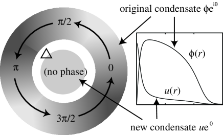
Fig.  5: The calculated wavefunctions $\phi(r)$ and $u(r)$ are showed in the right hand panel. They correspond to Figs. 1 and 4. The schematic figure of the phase change in the radial direction is drawn in the left hand panel. Because the new condensate without phase singularity appears at the center, the original vortex core (the triangle) must move outward.

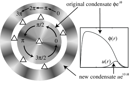
Fig.  6: The calculated wavefunctions $\phi(r)$ and $u(r)$ are shown in the right hand panel. They correspond to Figs. 1 and 4. The schematic figure of the phase change in the radial direction is drawn in the left hand panel. As the new condensate at large $r$ has large ($\sim 10\times 2\pi$ here) phase change, many vortex cores (the triangle) must appear.

3.3 Total energies — global stability

The comparison of the two energies in the systems with and without a vortex is another measure of the vortex stability. The comparison indicates the global stability of the vortex state relative to the non-vortex state. We calculate the critical $\Omega$ in which the energy of the system with the quantized vortex is equal to the system without a vortex under the same condition. We ignore the energy coming from the non-condensate part because the energy is 100 times smaller than the energy of the condensate in the present situation at $T=0$.

In the non-vortex state, the energy $E_{w=0}$ is not affected by the rotation $\Omega$, as is seen from eq. (17). The energy of the system without the vortex $E_{w=0}$, the energy of the singly quantized vortex system $E_{w=1}(\Omega)$, and the energy of system with the doubly quantized vortex $E_{w=2}(\Omega)$ are evaluated from eq. (21) as

$$E_{w=1}(\Omega)-E_{w=0}=h\nu N(0.22215-\Omega)$$ (22)

$$E_{w=2}(\Omega)-E_{w=1}(\Omega)=h\nu N(0.42071-\Omega).$$ (23)

Therefore, the critical $\Omega_{\rm global}$ where the two energies are equal; $E_{w=0}=E_{w=1}(\Omega)$ and $E_{w=1}(\Omega)=E_{w=2}(\Omega)$ are given by $\Omega_{\rm global}^{\rm L}=0.22215$ and $\Omega_{\rm global}^{\rm U}=0.42071$ for $an_{z}=55$. We call the stability defined by the energy crossing “global stability”.

3.4 Two stabilities

While the vortex stability in ⁴He systems is usually discussed in terms of the total energy (global stability in this paper), the stability in the present dilute BEC systems is discussed ${}^{\hbox{\immediate{?})}}$ using the lowest eigenvalue (local stability in this paper). These two stabilities are determined here and we can compare these quantitatively for a wide range of the parameter values of $an_{z}$.

The local stability is satisfied for $0.16085<\Omega<0.44610$ and the global stability is given by $0.22215<\Omega<0.42071$ when $an_{z}=55$. In the substantially wide $\Omega$ region the vortex state of the rotating BEC systems is stable locally and globally.

As mentioned previously, the system is characterized by the number $an_{z}$ and the rotation $\Omega$. In Fig. 7 we show four critical $\Omega$’s as a function of $an_{z}$. It is seen from Fig. 7 that as $\Omega$ increases, (1) the singly quantized vortex becomes stable locally first, (2) the energy of this vortex state is lower than that in the corresponding non-vortex state and the singly quantized vortex nucleates in the system, corresponding to (B) in Fig. 7, and (3) this single vortex state is kept stable up to either $\Omega^{\rm U}_{\rm global}$ or $\Omega^{\rm U}_{\rm local}$. These divide the parameter space into three regions: the vortex unstable region (A), the single vortex stable region (B) and the single vortex unstable region (C) where many vortices may appear.

Fig.  7: Phase diagram in the $\Omega$ vs $an_{z}$ plane, showing the three characteristic regions: the vortex unstable region (A), the single vortex stable region (B) and the single vortex unstable region (C) where many vortices may appear. Solid lines show $\Omega_{\rm global}$ and dotted lines show $\Omega_{\rm local}$. Upper two lines and lower two lines are $\Omega^{\rm U}$ and $\Omega^{\rm L}$ respectively.

4 Conclusion and Discussions

In order to obtain more insights into the vortex stability problem in the Bose-Einstein condensation of alkali atom gases confined in a harmonic potential, we have extended our previous work ${}^{\hbox{\immediate{?},\penalty 1000\hskip 0.91003pt plus 0.70004pt minus 0.70004pt{?})}}$ to the case where the cylindrical system is under forced rotation.

Our calculation is done within the framework of the non-selfconsistent Bogoliubov theory and yields the vortex stability phase diagram shown in Fig. 7. The stability of the vortex state is examined by the two different ways, that is, the local stability and the global stability. The previous cases ,${}^{\hbox{\immediate{?},\penalty 1000\hskip 0.91003pt plus 0.70004pt minus 0.70004pt{?})}}$ which are consistent with the present results, correspond to the $\Omega=0$ axis in this figure where the vortex is intrinsically unstable. This instability is seen to occupy a finite region, rather than the isolated line confined at $\Omega=0$ for various densities $n_{z}$ and the scattering lengths $a$.

We have examined not only the above intrinsic local stability, but also the global stability of the single vortex relative to the non-vortex state. This allows us to draw the whole perspective for the vortex stability problem. As is seen from Fig. 7, this global stability borderline $\Omega_{\rm global}^{\rm L}$ corresponding to the vortex nucleation is always situated above the intrinsic stability borderline $\Omega_{\rm local}^{\rm L}$. This means that for any $an_{z}$ values investigated the singly quantized vortex, which is nucleated, can exist as a (locally) stable object under rotation at $T$=0. It is to be noted that the present results in the non-selfconsistent calculations are applicable even for selfconsistent calculations such as the Popov approximation.

We have performed a similar study for the rigid wall case instead of the present harmonic potential case. Our data show the same vortex stability phase diagram for the system sizes up to 80$\times$(coherence length), confirming the previous conclusion ${}^{\hbox{\immediate{?})}}$ that the intrinsic vortex unstable region exists at a lower $\Omega$ region.

Together with the previous finite temperature calculations ,${}^{\hbox{\immediate{?})}}$ the present calculation concludes that alkali atom Bose gases in BEC can sustain and exhibit the stable vortex in appropriate temperatures and appropriate rotations.

References

- [1] M. H. Anderson, J. R. Ensher, M. R. Matthews, C. E. Wieman, and E.A. Cornell: Science, 269 (1995) 198.
- [2] C. C. Bradley, C. A. Sackett, J. J. Tollett, and R. G. Hulet: Phys. Rev. Lett. 75 (1995) 1687.
- [3] K. B. Davis, M.-O. Mewes, M. R. Andrews, N. J. van Druten, D. D. Durfee, D. M. Kurn, and W. Ketterle: Phys. Rev. Lett. 75 (1995) 3969.
- [4] See for recent experiments, C. J. Myatt, E. A. Burt, R. W. Ghrist, E. A. Cornell, and C. E. Wieman: Phys. Rev. Lett. 78 (1997) 586 and references therein.
- [5] D. S. Jin, J. R. Ensher, M. R. Matthews, C. E. Wieman and E. A. Cornell: Czech. J. Phys. 46 (1996) 3070; N. J. van Druten, C. G. Townsend, M. R. Andrews, D. S. Durfee, D. M. Kurn, M. -O. Mewes and W. Ketterle: Czech. J. Phys. 46 (1996) 3077.
- [6] F. Dalfovo, S. Giorgini, L. P. Pitaevskii, and S. Stringari: preprint (cond-mat/9806038).
- [7] W. F. Vinen: in Superconductivity ed. by R. D. Parks (Marcel Dekker, New York, 1969) Chapter 20.
- [8] R. J. Donnelly: Quantized Vortices in Helium II (Cambridge University, Press Cambridge, 1991) pp. 28, 53.
- [9] N. Bogoliubov: J. Phys. (USSR) 11 (1947) 23.
- [10] L. P. Pitaevskii: Zh. Eksp. Teor. Fiz., 40 (1961) 646 [English Transl. Sov. Phys. -JETP 13 (1961) 451].
- [11] A.L. Fetter: Phys. Rev. 138 (1965) A709, Phys. Rev. 140 (1965) A452, and Ann. Phys. (N. Y. ) 70 (1972) 67.
- [12] S. Sinha: Phys. Rev. A 55 (1997) 4325.
- [13] M. Edwards, R. J. Dodd, C. W. Clark, P. A. Ruprecht, and K. Burnett: Phys. Rev. A 53 (1996) R1950.
- [14] F. Dalfovo and S. Stringari: Phys. Rev. A 53 (1996) 2477.
- [15] R. J. Dodd, K. Burnett, M. Edwards, and C. W. Clark: Phys. Rev. A 56 (1997) 587.
- [16] D. S. Rokhsar: Phys. Rev. Lett. 79 (1997) 2164; preprint(cond-mat/9709212).
- [17] K.-P. Marzlin and W. Zhang: Phys. Rev. A 57 (1998) 3801; 57(1998) 4761 .
- [18] B. Jackson, J. F. McCann, and C. S. Adams: Phys. Rev. Lett. 80 (1998) 3903.
- [19] A. A. Svidzinsky and A. L. Fetter: preprint (cond-mat/9803181).
- [20] A. L. Fetter: preprint (cond-mat/9808070).
- [21] T. Isoshima and K. Machida: J. Phys. Soc. Jpn., 66 (1997) 3502.
- [22] T. Isoshima and K. Machida: preprint (cond-mat/9807250) (to be published in Phys. Rev. A).