Spectral correlations in systems undergoing a transition from periodicity to disorder

Abstract

We study the spectral statistics for extended yet finite quasi 1-d systems which undergo a transition from periodicity to disorder. In particular we compute the spectral two-point form factor, and the resulting expression depends on the degree of disorder. It interpolates smoothly between the two extreme limits – the approach to Poissonian statistics in the (weakly) disordered case, and the universal expressions derived in [2] and [1] for the periodic case. The theoretical results agree very well with the spectral statistics obtained numerically for chains of chaotic billiards and graphs.

I Introduction

The spectrum of an unbounded periodic system is arranged in continuous bands and the corresponding eigenfunctions are extended (unnormalisable). When sufficient disorder is introduced, the system is Anderson localised - the spectrum is point like and the eigenfunctions are localised (normalisable). The transition from a continuous to a point spectral measure is a drastic effect, which might have been used to characterize the transition. However, this approach is of a limited value, since in practice one always deals with finite systems, where the spectral measure is point-like both in the periodic and in the disordered situations. In finite systems, the mean spectral density is independent of the degree of disorder. Therefore, for finite systems, the effect of disorder on the energy spectrum can be discerned only in the spectral correlations. Indeed, this approach to the characterization of the Anderson transition in three dimensional systems was used [3], and the spectral measures were shown to undergo an abrupt change when the critical level of disorder is reached. In the present paper we study the spectral statistics for finite quasi 1-d systems which undergo a transition from periodicity to disorder. (Quasi 1-d disordered systems of finite length can be either “metallic” or “insulating” depending on whether the localization length is larger or smaller than the system length. We shall consider only the first case, and the strength of the disorder will be restricted accordingly, to the range of values which is sometimes called weak disorder). We shall focus our attention to the spectral two-point form factor, and show that it depends very sensitively on the degree of disorder, and derive a universal expression, which interpolates continuously between the periodic and the disordered yet metallic limits.

The spectral form factor is the main object of our discussion, and it is defined in the following way. The spectrum is unfolded by introducing the dimensionless energy $\epsilon$, through the relation ${\rm d}\epsilon=\langle d\rangle(E)\,{\rm d}E$ where $\langle d\rangle(E)$ is the mean spectral density. The corresponding dimensionless time $\tau$ measures time in units of the Heisenberg time $t_{\rm H}=2\pi\hbar\langle d\rangle$. We consider a finite spectral interval of length $\Delta\epsilon$ centered at $\epsilon_{\rm c}$, and denote its characteristic function by $\chi(\epsilon-\epsilon_{\rm c})$. Since the mean spectral density of the unfolded spectrum is unity, the number of states in the interval $\Delta\epsilon$ is ${\cal N}=\Delta\epsilon$. This energy interval should be sufficiently large so that ${\cal N}\gg 1$, and sufficiently small so that the mean level density and the classical dynamics do not change much as the energy is scanned across it. The oscillatory part of the spectral density in this interval is

$$\widetilde{d}(\epsilon)=\chi(\epsilon-\epsilon_{\rm c})\left[\sum_{q}\delta(\epsilon-\epsilon_{q})-1\right].{}$$ (1)

The Fourier transform of this function is

$$d_{c}(\tau) = \int\mbox{e}^{-2\pi{\rm i}\epsilon\tau}\widetilde{d}(\epsilon)\ {\rm d}\epsilon$$ (2)

$$= \sum_{q}\chi(\epsilon_{q}-\epsilon_{\rm c})\,\mbox{e}^{-2\pi{\rm i}\epsilon_{q}\tau}-\delta_{\Delta\tau}(\tau)\ .$$ (3)

The Fourier transform of the normalized characteristic function is denoted by $\delta_{\Delta\tau}(\tau)$ and its width is $\Delta\tau\sim 1/\Delta\epsilon$. The form factor is expressed as

$$K(\tau)={1\over{\cal N}}\langle|d_{c}(\tau)|^{2}\rangle_{c}.$$ (4)

We use $\langle\cdot\rangle_{c}$ to denote the spectral average, which is taken over the non overlapping energy intervals located about a set of $\epsilon_{c}$ values. One can also perform the averaging over any free parameter of the system or over disorder when it is introduced. It can be easily shown that (4) is nothing but the Fourier transform of the spectral two-point correlation density [8]. For a discrete spectrum the normalization in (4) is such that the form factor approaches a constant $\gamma$ as $\tau\to\infty$ where $\gamma$ is the mean spectral degeneracy.

The expressions for the spectral form factors in the extreme situations of exact periodicity and weak disorder are known. In the latter case, when the length of the system does not exceed the localization length, and assuming that the Heisenberg time is shorter than the Thouless time the spectral statistics takes the form [6]

$$K(\tau)=\left\{\begin{array}[]{ll}g_{\rm T}\sqrt{\tau/2c}&{\rm for}\ \ \ \tau<1\\ 1&{\rm for}\ \ \ \tau>1\ \ .\end{array}\right.$$ (5)

The factor $g_{T}$ can take the values $1$ or $2$ depending on whether time reversal invariance is respected or violated, and $c$ is the conductivity of the chain. The spectral form factor for periodic systems was recently derived using both field-theoretical methods [2] and the semiclassical approximation [1]. Since the latter theory is the basis for the approach developed in the present paper, we shall describe it briefly to introduce the concepts and the notations which will be used in the sequel.

We consider a chain of $N$ identical chaotic unit cells of length $a=1$, with periodic boundary conditions, such that the full system shows a discrete translation invariance (Fig. 1(a)). (Alternatively, we could discuss a disordered ring configuration which is threaded by an Aharonov-Bohm flux line. This is the system analyzed in [2]). In such a system, the classical evolution within a unit cell becomes ergodic after a short time, and one can approximate the classical evolution in the entire chain by diffusive evolution. We shall denote the diffusion constant by $D$. The time it takes the diffusive evolution to cover the phase-space uniformly is the Thouless time.

Due to translation invariance, the quantum spectrum consists of discretised energy bands whose width depends on the (dimensionless) conductivity per unit cell. It is defined as $c_{1}=2\pi\hbar\langle d_{1}\rangle D/a^{2}$, where $\langle d_{1}\rangle$ is the mean level density per unit cell. A few examples of typical bands are shown in Fig. 2. One can see that for low $c_{1}$, the bands are flat and show little structure. For high values, the bandwidth is of the order of the inter-band spacing, and the bands can hardly be recognized if the discretisation is too coarse.

If the system under discussion is invariant under an anti-unitary symmetry (such as e.g., time-reversal) the bands are symmetric about the center and the edges of the Brillouin zone, and the levels are doubly degenerate ($\gamma=2$). The reflection symmetry and the degeneracies are broken if the symmetry is lifted, and in this case $\gamma=1$.

The quantum spectrum is characterized by two energy scales, the mean intra-band spacing and the mean inter-band spacing. The ratio between them is at least $N$, the number of unit cells. We are interested here in the large $N$ limit, and therefore these energy scales are very well separated. Since $\langle d\rangle\approx\langle d_{1}\rangle N$, the spectral correlations which pertain to the inter-band scale affect the behavior of the form factor in the range $0<\tau<1/N$. The correlations between levels in the same band leave their mark on $K(\tau)$ in the domain $1/N<\tau<1$. The fact that the spectrum is composed of discrete (possibly degenerate) energy levels is expressed in the spectral form factor in the domain $1<\tau$, where the form factor approaches the constant value $\gamma$.

We used different approximations to express the form factor in the three domains mentioned above [1].

• $0<\tau<1/N\$: Here one starts from the semiclassical trace formula [5] and employs the “diagonal approximation” [4] to write

  $$K(\tau)\approx g_{\rm T}N\tau P(\tau)\ .$$ (6)

  The factor $N$ is due to the discrete translation symmetry, because of which any generic periodic orbit is replicated $N$ times in the system. $g_{\rm T}$ stands for the classical degeneracy due to time-reversal (or any other anti-unitary) symmetry and it can take the values $1$ or $2$. $P(t)$ is the classical probability to stay in the same unit cell from which the trajectory started, after the time $t=\tau t_{H}$ [6]. Because phase-space is covered diffusively, $P(t)\approx({1\over 2\pi Dt})^{1/2}$ and hence,

  $$K(\tau)\approx g_{\rm T}N\sqrt{N\tau/2c_{1}}\ ,$$ (7)

  where $c_{1}$ is the dimensionless conductivity per unit cell which was introduced above.

• $1/N<\tau<1\$: As $\tau$ increases, the form factor provides information on a finer energy scale. In the vicinity of $\tau=1/N$, the energy levels within a single band cannot be resolved, hence $K(\tau\approx 1/N)$ takes a value which is proportional to the apparent degeneracy $N$. Finer details of the energy correlation inside the band are manifested for larger values of $\tau$. To understand the behavior of the spectral form factor, one writes the levels in the band $\beta$ as $\epsilon_{\beta}(q)\ ,\ q=1,\ldots,N$, and substitutes in (4). Neglecting the cross-band correlations one gets

  $$K(\tau)=\left\langle\ {1\over N}\left|\sum_{q=1}^{N}{\rm e}^{-i2\pi\epsilon_{\beta}(q)\tau}\right|^{2}\ \right\rangle_{\beta}$$ (8)

  This is the spectral form factor for a band, averaged over all the bands. The $q$ summation can be performed by the saddle-point (or the uniform) approximation. The main contribution comes from the vicinity of the band extrema which correspond to the energy values where the spectral density is singular. That is, the prominent features in the form factor are due to the Van Hove singularities. Denoting by $\partial^{2}_{q}\epsilon_{\beta}$ the second derivative of the band function at its extrema, one gets

  $$K(\tau)=C\left\langle(\partial^{2}_{q}\epsilon_{\beta})^{-1}\right\rangle_{\beta}\tau^{-1},$$ (9)

  where $C$ is a numerical constant. It was shown in [1] that the values of the constants which appear in (7) and in (9) are compatible so that the two expressions match at $\tau=1/N$.

• $\tau>1\$: The time interval is sufficient to resolve the point-like character of the spectrum. Hence,

  $$K(\tau)=\gamma\ .$$ (10)

In the following sections we shall study how the expressions ( 7,9,10 ) make the transition to the Poisson form factor $K(\tau)=1$ as disorder is introduced. The semiclassical (diagonal) approximation will be the starting point for the discussion of the transition in the first domain. This will be done in section II. To investigate $K(\tau)$ in the second and the third domains, it suffices to study a system which has a single band in the periodic limit. The $N$–site periodic Anderson model is such a system, and it will be discussed in section III. The important observation made in this section is that the transition is well described by considering the disorder perturbatively. The resulting explicit formulae for $K(\tau)$ in the transition regime, reproduce the numerical data extremely well. The perturbative treatment also sheds light on the peculiar mechanism which reduces the value of $K(\tau)$ from $\gamma$ to $1$ in the third domain when the disorder splits up the degeneracies of the spectrum. We shall compare the results obtained separately for the three domains with numerical data for billiard and graph (network) systems. This will be done in section IV, where we shall summarize and discuss our findings.

II Introducing disorder – the semiclassical approximation

We shall compute the spectral form factor (4) in terms of the Fourier transform of the oscillatory part of the spectral density. Using Gutzwiller’s trace formula, $d(\tau)$ can be expressed semiclassically as a sum over the periodic orbits $j$ of the system

$$d(\tau)=\sum_{j}\delta_{\Delta\tau}(\tau-\tau_{j})\;\tau_{j}\,A_{j}\,\mbox{e}^{{\rm i}\,s_{j}}$$ (11)

with primitive period $\tau_{j}\approx\tau$. $A_{j}$ denotes the weight of the orbit corresponding to its stability and includes the Maslov phase. $s_{j}$ is the action of the orbit in units of $\hbar$. Following the standard approximation, we neglect the contribution of repetitions of primitive orbits to the sum (11). The form factor is now given by a double sum over periodic orbits

$$K(\tau)={1\over\Delta\epsilon}\left\langle\sum_{j,j^{\prime}}\delta_{\Delta\tau}(\tau-\tau_{j})\,\delta_{\Delta\tau}(\tau-\tau_{j^{\prime}})\,A_{j}A^{*}_{j^{\prime}}\,\mbox{e}^{{\rm i}\,(s_{j}-s_{j^{\prime}})}\right\rangle\,.$$ (12)

It is well known [4], that for short time $\tau$ this sum can be restricted to the diagonal terms $j=j^{\prime}$. However, when due to a symmetry, the orbit appears in $g_{j}$ different but symmetry-related versions, the contribution of all the symmetry-conjugated orbits must be added coherently. In such cases, (12) reduces within the diagonal approximation to

$$K(\tau)\approx\sum_{j}g_{j}\,\delta_{\Delta\tau}(\tau-\tau_{j})\,\tau_{j}\,|A_{j}|^{2}\,.$$ (13)

In the case of an extended, nearly periodic system, the diagonal approximation is valid up to $\tau=1/N$, the Heisenberg time of the unit cell [8].

¿From very general arguments it is clear, that in a system whose phase-space decomposes into several equivalent subspaces related by (unitary as well as anti-unitary) symmetry, the mean degeneracy $g$ is just the number of such subspaces. Thus, if time-reversal invariance is the only symmetry obeyed, phase-space points with opposite momenta are equivalent and consequently phase-space is partitioned in $g_{\rm T}=2$ subspaces. In our problem, phase-space is invariant under a symmetry group containing $N$ elements and therefore $g=Ng_{\rm T}$. Using the sum rule for periodic orbits [9, 6], the form factor is finally written as

$$K(\tau)\approx g_{\rm T}N\tau\,P(\tau)\ .$$ (14)

which we introduced in the previous section (6). The normalisation of the staying probability $P(\tau)$ is such that $P(\tau)=\Omega/\omega(\tau)$ at a time $\tau$, where the classical flow covers ergodically the part $\omega(\tau)$ of the total energy-shell volume $\Omega$. In particular, $P(\tau\to\infty)=1$ for an ergodic system and $P(\tau)=N$ in a system which is composed of $N$ unconnected ergodic cells. A more precise definition can be found in [6, 7, 8]. For the present purpose, we need only the following property [8]: the return probability for a system composed of chaotic unit cells is independent of the presence or absence of long-range spatial order. Thus, within the diagonal approximation, the only effect of the introduction of disorder is the destruction of the coherence between the contributions of orbits which were related by symmetry in the original periodic system. This implies that in the diagonal approximation for $K(\tau)$, (see (14)) $g=Ng_{\rm T}$, is to be replaced by $g=g_{\rm T}.$

In order to describe the transition from $g=Ng_{\rm T}$ to $g=g_{\rm T}$ as the spatial symmetry is broken, we go slightly beyond the diagonal approximation (13) in that we retain in Eq. (12) the off-diagonal contributions from all those orbits which are degenerate in the symmetric system

$$K(\tau)\approx g_{\rm T}\sum_{r}\delta_{\Delta\tau}(\tau-\tau_{r})\,\tau_{r}\,|A_{r}|^{2}\,\left|\sum_{j,j^{\prime}=1}^{N}\mbox{e}^{{\rm i}\,(\Delta s_{r,j}-\Delta s_{r,j^{\prime}})}\right|^{2}\,.$$ (15)

$r$ runs now over all groups of symmetry-related orbits, while $j,j^{\prime}$ label the $N$ orbits within each group. Possible degeneracies due to time-reversal are not affected by breaking the spatial symmetry and are thus contained in the prefactor $g_{\rm T}$. The disorder which breaks the symmetry has been assumed weak enough such that (i) the orbits within the Heisenberg time of the unit cell $\tau_{r}<1/N$ are structurally stable, i. e. no (short) periodic orbits appear or disappear due to the disorder, and (ii) the disorder does not alter by much the stability amplitudes and the periods within a group $r$ so that in the prefactor $A_{r,j}\approx A_{r}$, $\tau_{r,j}\approx\tau_{r}$. The variation of the actions are of the same order, but they cannot be neglected because they are measured in units of $\hbar$ and therefore, the resulting changes in phase, $\Delta s_{r,j}$ should be taken into account.

Comparing (13) and (15) we see that Eq. (14) represents the form factor also in the case of a weakly broken spatial symmetry, if $g$ is replaced by an effective degeneracy

$$g(\tau,\delta) = {g_{\rm T}\over N}\left\langle\sum_{j,j^{\prime}=1}^{N}\mbox{e}^{{\rm i}\,(\Delta s_{r,j}-\Delta s_{r,j^{\prime}})}\right\rangle_{r}$$ (16)

$$= {g_{\rm T}\over N}\left(N+\left\langle\sum_{j\neq j^{\prime}}\mbox{e}^{{\rm i}\,(\Delta s_{r,j}-\Delta s_{r,j^{\prime}})}\right\rangle_{r}\right)$$ (17)

which depends on the time $\tau$ since the average on the r. h. s. is over all groups of periodic orbits $r$ with length $\tau_{r}\approx\tau$. The dimensionless parameter $\delta$ has been introduced to characterize the strength of the symmetry-breaking disorder in a way to be specified in Eq. (18) below.

In order to evaluate Eq. (16), we need some information about the distribution of the disorder contributions to the phases of the periodic orbits $\Delta s_{r,j}$. We assume, that the correlation length of the disorder is negligibly small compared to the mean length of an orbit. In this case $\Delta s_{r,j}$ is a sum of many independent contributions, and the number of these contributions is proportional to the period of the orbit $\tau$. Hence, according to the central limit theorem, $\Delta s_{r,j}$ are independent Gaussian random variables with mean value $\langle\Delta s\rangle=0$ and variance

$$\langle\Delta^{2}s\rangle=\delta^{2}\tau\,,$$ (18)

where the average is over all orbits of period $\tau$. With these assumptions we find from (16)

$$g(\tau,\delta) = {g_{\rm T}\over N}\left(N+N(N-1)\left|\langle\mbox{e}^{i\Delta s}\rangle\right|^{2}\right)$$ (19)

$$= g_{\rm T}(1+[N-1]\,\mbox{e}^{-\delta^{2}\tau})\,.$$ (20)

In the first line we have used the fact that the $N\gg 1$ together with the statistical independence of $\Delta s_{r,j}$ and $\Delta s_{r,j^{\prime}}$ justified above to replace the sum over $j,j^{\prime}$ by its averaged value. In the second line, the Gaussian distribution of $\Delta s$ was employed to give $\langle\mbox{e}^{{\rm i}\Delta s}\rangle=\mbox{e}^{-\langle\Delta^{2}s\rangle/2}$. It is easy to see, that Eq. (16) indeed interpolates between $g=Ng_{\rm T}$ and $g=g_{\rm T}$ as a function of the disorder. Note that the parameter which characterizes the disorder, $\delta^{2}$, is multiplied by the time $\tau$ over which the disorder acts. Hence, the classification of the disorder as “weak” or “strong” depends on the relevant time scale.

In summary, we get,

$$K(\tau,\delta)=g_{\rm T}(1+[N-1]\,\mbox{e}^{-\delta^{2}\tau})\tau\,P(\tau)=g_{\rm T}(1+[N-1]\,\mbox{e}^{-\delta^{2}\tau})\sqrt{N\tau/2c_{1}}\ \ ;\ \ \tau<1/N\ .$$ (21)

This expression provides the smooth transition from the periodic case, via the weakly disordered to the “metallic” domain. In section IV we shall show that this simple formula reproduces the form factor in the transition from periodicity to disorder very well. We emphasize once again that the present theory does not describe strongly disordered systems where the localization length is shorter than the system size. Such systems are outside of the scope of the present approach which is based on the “diagonal” approximation.

III Introducing disorder - perturbation of a model with a single band

As explained in the introduction, the form factor in the domain $\tau>1/N$ is sensitive to the correlations among the levels which belong to the same band. Therefore, in order to investigate the form factor in this region, it is sufficient to study a model with a single band, which is what we do in the present section. In order to use the results of this section in the general context, we have to remember that the form factor in realistic systems is obtained as an average over many bands (see (8)). This will smooth out several features of the single-band form factor, as will be explained in the sequel.

The system we consider is a chain of $N$ unit cells of length $a=1$, with periodic boundary conditions at the end of the chain. The chaotic scattering process in each cell is represented by a random potential and the dynamics is discretised on a lattice. Choosing convenient units, the Schrödinger equation reads

$$-\left(\phi_{n+1}-2\phi_{n}+\phi_{n-1}\right)+V_{n}\phi_{n}=E\phi_{n},\quad\phi_{n}=\phi_{L+n},$$ (22)

where $\phi_{n}$ is the wave function on the $n$th site. The on–site potentials $V_{n}$ are uncorrelated, random variables which are picked out from the same Gaussian distribution function with variance $\sigma$. They obey

$$\langle V_{n}\rangle = 0,\quad\langle V_{n}V_{m}\rangle=\delta_{nm}\sigma^{2}\qquad n,m=0\ldots N-1,$$ (23)

The complexity of the scattering process is incorporated by neglecting the correlations between the potentials on different sites.

In the periodic limit ($\sigma=0$), the levels are arranged in a discrete band

$$E_{q}^{0}=2(1-\cos(2\pi q/N))\;\;\;q=0,...,N-1.$$ (24)

The level density (compare Eq. 1)

$$d(E)=\sum_{q=0}^{N-1}\delta(E-E_{q})$$

exhibits van Hove singularities at the band edges $E=0$ and $E=4$. This is a direct consequence of the periodicity of the system.

For $\sigma\neq 0$ the singularity is smoothed out and for large values of $\sigma$ the level density becomes uniform between the upper and lower ends of the spectrum. This is the typical behavior we expect in generic one-dimensional disordered systems. ¿From here on we consider the periodic case as the limit of the disordered system when $\sigma\rightarrow 0$. Accordingly, levels can be unfolded with the constant density. Since we consider here only weak disorder the mean level density is taken as

$$\langle d\rangle\approx N/4.$$ (25)

The spectral form factor was defined in (4). In the periodic case the energies are given by (24). The spectral form factor is

$$K(\tau,\sigma=0)=\frac{1}{N}\left|\sum_{q=0}^{N-1}\exp(-i\pi E_{q}^{0}\tau N/2)\right|^{2},$$ (26)

The second argument of the form factor denotes the strength of the disorder, and in the present periodic case it is $0$. The expression (26) can be rewritten by expanding the exponential into a Bessel series:

$$e^{iN\tau\pi\cos{\frac{2\pi}{N}q}}=\sum_{k=-\infty}^{\infty}i^{k}e^{iq\frac{2\pi}{N}k}\cdot J_{k}(\pi N\tau)$$ (27)

Exchanging the order of the summation over $q$ and $k$ yields

$$K(\tau,0)=N\left|J_{0}(\pi\tau N)+2\sum_{n=1}^{\infty}i^{nN}J_{nN}(\pi\tau N)\right|^{2}.$$ (28)

The function $K(\tau,0)$ which is shown in Fig. 7 displays different features in the three domains of $\tau$. In the domain $0\leq\tau\leq 1/N$ the first term in (28) is dominant and $J_{0}(\pi\tau N)\approx 1$. Hence, the form factor assumes the constant value $N$, and does not show any structure at all because we are dealing with a model with a single band. At $\tau>1/N$, the form factor is a highly irregular function. It fluctuates more rapidly with increasing number of sites $N$. However, in order to compare the present theory with results which are derived for realistic systems, one should remember that in the latter case, the form factor is averaged over many bands which differ in their widths and structure. Such averaging can be effectively achieved by smoothing $K(\tau,0)$ over a small $\tau$ window.

The smoothed form factor $\langle K(\tau,0)\rangle_{\tau}$ is shown in Fig. 7. In the range $1/N<\tau<1/\pi$ (28) is dominated by the Bessel function with zero index. The average behavior for large $N$ and $\tau<1/\pi$ can be approximated as

$$\langle K(\tau,0)\rangle_{\tau}\approx N\langle\left|J_{0}(\pi\tau N\right|^{2}\rangle_{\tau}\approx\frac{1}{\pi^{2}\tau},$$ (29)

where we used the asymptotic form of the Bessel function

$$J_{\nu}(z)\approx\sqrt{\frac{2}{z\pi}}\cos(z-\nu\pi/2-\pi/4)$$

and the average $\langle\cos^{2}\rangle_{\tau}=1/2$.

In the third domain, $\tau>1/\pi$, the window-averaged function $\langle K(\tau,0)\rangle_{\tau}$ converges to a constant value. This constant is $\gamma$, the average degeneracy of the levels, and it approximately equals $2$ since most levels are doubly degenerate (except $E_{0}=0$ and also $E_{N/2}=4$ if $N$ is even). In this range of $\tau$ values, all Bessel functions contribute. Resumming the asymptotic forms of the Bessel functions we get

$$\langle K(\tau,0)\rangle_{\tau}\approx 2$$ (30)

We conclude from this discussion that the one-band model, after proper averaging, reproduces the expected features of $K(\tau,0)$ in the relevant range $\tau>1/N$.

Introducing disorder, the form factor is given by

$$K(\tau,\sigma)=\frac{1}{N}\left\langle\left|\sum_{q=0}^{N-1}\exp(-i\pi E_{q}^{\sigma}\tau N/2)\right|^{2}\right\rangle_{\sigma}$$ (31)

where $\langle\ldots\rangle_{\sigma}$ represents the average over the disorder and $E_{q}^{\sigma}$ are the eigenenergies of the Eq.  (22) with $\sigma\ll 1$.

In the case of weak disorder, we can use degenerate perturbation theory to calculate how doubly degenerate energy levels are split. In first order the eigenenergies are given by

$$E_{\pm q}^{\sigma} \approx E_{\pm q}^{0}\pm\frac{1}{N}\left|\sum_{n=0}^{N-1}V_{n}\exp(\pm i2\frac{2\pi}{N}qn)\right|\quad\mbox{for}\quad q\neq 0,N/2$$ (32)

$$\approx E_{q}^{0}\quad\mbox{for}\quad q=0\mbox{ (and q=N/2 if N is even)}.$$ (33)

Here we ignored a $q$–independent constant, since it does not affect the form factor. The main effect of the perturbation is that it breaks the degeneracy of the energy levels which are symmetrically placed about the center of the band. The change of the mean level spacing is small, and can be neglected to leading order.

Substituting the perturbed energy levels into (31) and leaving out the unimportant $q=0$ (and $q=N/2$ if $N$ is even) levels we have

$$K(\tau,\sigma) \approx \frac{1}{N}\left|\sum_{q=1}^{\frac{N-1}{2}}2e^{-\pi iE_{q}^{0}\tau N/2}\cos\left(\frac{1}{2}\left|\sum_{n=0}^{N-1}V_{n}e^{\left(i2\frac{2\pi}{N}qn\right)}\right|\pi\tau\right)\right|^{2}\ .$$ (34)

The disorder averaging can be performed analytically, as described in the appendix. For large $N$ it leads to

$$K(\tau,\sigma)=1+A(2\alpha)+A^{2}(\alpha)(K(\tau,0)-2),$$ (35)

where the universal function $A(\alpha)$ is defined in the appendix. A new combination of the variables involving the disorder strength shows up in this expression

$$\alpha=\frac{\pi\tau\sigma\sqrt{N}}{2},$$ (36)

governing the properties of the transition from the periodic to the disordered case. For large $\tau$ values the form factor converges to $1$, since the perturbation breaks the degeneracy of the levels of the periodic system. Please note that–as in the semiclassical result Eq. (19)– the deviation from the periodic form factor is governed by a dimensionless parameter containg the product of disorder strength and time.

Approximating $K(\tau,0)$ by its average (29) yields

$$\langle K(\tau,\sigma)\,\rangle_{\tau}\approx\left\{\begin{array}[]{ll}(1-e^{-\alpha^{2}})^{2}+{e^{-\alpha^{2}}\over\pi^{2}\tau}&\mbox{for\ \ }\tau<1/\pi\\ 1+A(2\alpha)&\mbox{for\ \ }\tau>1/\pi\end{array}\right.\ .$$ (37)

The $\tau<1/\pi$ part describes how the band structure is destroyed while the $\tau>1/\pi$ part describes how the double degeneracy of levels is resolved (see Fig.8).

We can interpret the result for $\tau>1/\pi$ in terms of the distribution $p_{\sigma}(s)$ of splittings of levels $s=E_{q}^{\sigma}-E_{-q}^{\sigma}$ which are degenerate in the periodic case. For large $\tau$ the form factor is the Fourier transform of this distribution:

$$K(\tau,\sigma)=1+\int_{0}^{\infty}dsp_{\sigma}(s)\cos(s\tau\pi N/2).$$ (38)

Using the derived expression (59) for $A(\alpha)$, we can conclude that the splitting distribution has the form

$$p_{\sigma}(s)=\delta\cdot p_{W}(s\delta),$$ (39)

where $p_{W}(s)=\pi se^{-\pi s^{2}/4}/2$ is the Wigner surmise and $\delta=\sigma\sqrt{N}$ is the mean splitting of levels. The Wigner surmise is known to be the exact distribution of the difference of the two eigenvalues of a $2\times 2$ GOE random matrices. We can conclude that in the present case, the ensemble of $2\times 2$ matrix describing the splitting of levels in the first-order degenerate perturbation theory, reproduces the spacing distribution of the corresponding GOE with mean level spacing $\delta$.

To check the applicability of the leading order perturbation theory, we computed the form factor numerically and compared with the analytical result. The parameter range was $\sigma=0.002\ldots 0.256$ and $N=32\ldots 256$. The numerical results has been averaged for 1000 different disorder realizations. In Fig. 8 we compare formula (35) and the simulations. We have found surprisingly good agreement in the whole range of $\tau$. The fact that $K(\tau)$ displays a minimum where its value is less than $1$, and that it approaches $1$ asymptotically from below, is a direct consequence of the Wigner distribution of level splittings. In the next section we shall show that this formula applies very well also in the case of a multi-banded spectrum, indicating that the splitting distribution follows the Wigner distribution in more complicated situations too.

IV Comparison with numerical results and Discussion

A A chain of chaotic billiards

The first class of systems which were investigated numerically are chains of chaotic billiards, (see Fig. 1) which can be arranged in a periodic (Fig. 1(a)) or a disordered (Fig. 1(b)) fashion. We denote the size of an individual billiard (i.e., the unit cell in the periodic case) by $a$ and the chain length by $L$ (and $N=L/a\gg 1)$. In the following we discuss weakly disordered chains and assume that the conductance of the chain $c=Nc_{1}\stackrel{{\scriptstyle>}}{{\sim}}1$. On time scales larger than the classical ergodic time for a single cell, the classical dynamics in the chain of billiards is diffusive, characterized by the diffusion constant $D$. In the diffusive regime, the classical dynamics of the system, and hence the diffusion constant, are, to a good approximation, independent of the strength of the disorder. The correlations in the quantum spectrum, however, crucially depend on whether the system is periodic or not, as discussed above.

In this section we present numerical results for the form factor $K(\tau)$ in weakly disordered chains. The case of periodic chains was analyzed in detail in two previous publications [1]. Here we focus on the crossover from the periodic case to the weakly disordered (metallic) case, which is predicted to follow (21) as a function of the disorder parameter $\delta$. Due to time-reversal invariance of the billiard chain, $g_{\rm T}=2$.

We have considered a chain composed of unit cells as shown schematically in Fig. 3. The sizes of the half disks were chosen so that the contribution of direct trajectories to the conductance is minimized. Disorder was introduced by shifting the disks at random to the right or to the left by a small amounts $\Delta x$. The dimensionless variance $\langle(\Delta x)^{2}\rangle$ is a measure of the disorder strength.

Consider a periodic orbit $j$ which hits $M$ disks, $m=1,\ldots,M$. Its action $s_{j}$ (measured in units of $\hbar$) is affected by the $M$ shifts $\Delta x_{m}$ and changes by an amount $\Delta s_{j}$, It is plausible that $\langle\Delta^{2}s_{j}\rangle\propto\langle(k\Delta x)^{2}\rangle\,\tau$ and thus

$$\delta^{2}=C_{d}\langle(k\Delta x)^{2}\rangle\,.$$ (40)

We have used (40) to estimate the quantity $\delta^{2}$ in (21). The constant of proportionality $C_{d}$ in (40) remains undetermined, it depends on the geometry of the system and on $k$.

We have performed quantum-mechanical calculations for systems composed of $N=16$ unit cells, with disorder parameters covering the domain of applicability of (21). The quantum-mechanical wave functions satisfy the Helmholtz equation augmented with Dirichlet boundary conditions on the channel walls and periodic boundary conditions along the chain. The quantum spectrum of this system can be determined using the method described in [1]. In this way we have obtained the quantum spectra for several realizations of disorder, as well as for the periodic chain.

Fig. 4 summarizes the results of our numerical calculations. It shows $K(\tau,\delta)$ as a function of $\tau$, in the periodic case, for weakly broken periodicity (four different disorder strengths) and for weak disorder. The conductivity per unit cell is independent of the disorder, and its numerical value was determined from a simulation of the classical dynamics of the system. A fit to the diffusion propagator at times larger than the ergodicity time allows one to determine $D$ from which $c_{1}\simeq 33$ emerges. The calculations were conducted for 6 values of the disorder strengths $\Delta^{2}\equiv\langle k^{2}(\Delta x)^{2}\rangle=0.0,\ 6.87\times 10^{-4},\ 9.55\times 10^{-4},\ 1.49\times 10^{-3},\ 2.56\times 10^{-3}{\rm and}\ 4.38\times 10^{-3}$. In all cases, we have calculated $K(\tau)$ from 1500 eigenvalues, in the domain of $k$ values which support $28$ open transverse channels.

The semiclassical theory for the periodic case reproduces the numerical results uniformly well over the three ranges of $\tau$ values. The semiclassical theory matches very well the numerical results for the disordered systems in the domain $\tau<1/N$. However, the numerical results in the domain $1/N<\tau<1$ are not sufficiently smooth to allow a meaningful comparison with the theory developed in section (III). In this domain, the spectrum is afflicted by frequent near–degeneracies which make the calculation rather costly in terms of computer resources. This problem is circumvented in the periodic case, where the translational invariance is used to facilitate the calculations. For larger values of the disorder, the degeneracy disappears, but, the effect we are interested in disappears, too. In the next subsection we discuss a different model exhibiting a transition from periodicity to weak disorder, where a quantitative comparison in the transition regime is possible.

B A chain of quantum graphs

In this section we investigate a second model system—quantized graphs which were recently shown to provide an excellent example for a quantum chaotic system [10]. The graphs are defined by $v=1,\dots,V$ vertices and $b=1,\dots,B$ bonds with lengths $L_{b}$ connecting them. The wave function on a graph is a $B$-component function $\left(\psi_{1}(x_{1}),\cdots,\psi_{B}(x_{B})\right)^{T}$. Each component satisfies the Schrödinger equation ($\hbar=2m=1$)

$$\left({{\rm d^{2}}\over{\rm d}x_{b}^{2}}+k^{2}\right)\psi_{b}(x_{b})=0\,.$$ (41)

At the vertices, the wave function must satisfy boundary conditions which impose continuity and current conservation. They guarantee that the Schrödinger operator is self adjoint, and its spectrum consists of discrete points. Implementing the boundary conditions, one derives a secular equation which provides a convenient means to compute the spectrum numerically. The graph is essentially a one-dimensional system, and therefore, the mean (wave number) spectral density is constant, proportional to the total length of the graph.

The graph representing one unit cell was chosen to be the “cylindrical” network shown in the inset of Fig. 5. The cylinder consists here of $n_{x}=2$ layers with $n_{y}=4$ vertices each. The unit cell was constructed from more than one layer in order to remove any residual symmetry. Two bonds lead from each vertex to the neighboring layers, two more to other vertices in the same layer. Hence we have for the unit cell $V=n_{x}n_{y}$ and $B=2n_{x}n_{y}$. The lengths of all bonds are random, but the total length of the graph was fixed at $L_{\rm H}=2\pi$ such that the mean length of a bond is $\bar{L}=\pi(2N\,n_{x}n_{y})^{-1}$ and the mean level spacing with respect to the wave number $k$ is unity. For this reason it is natural to use, instead of energy and time, the wave number $k$ and the length $l$ as conjugate variables, since then no unfolding is necessary. In complete analogy to (4) we introduce the spectral form factor via the length spectrum of the oscillating spectral density $\widetilde{d}(k)=\sum_{q}\delta(k-k_{q})-1$ using a rectangular window

$$K(\tau)={1\over\Delta k}\langle\left|d(\tau)\right|^{2}\rangle\,,$$ (42)

$$d(\tau)=\int_{k-\Delta k/2}^{k+\Delta k/2}{\rm d}k^{\prime}\mbox{e}^{-2\pi{\rm i}k\tau}\widetilde{d}(k)\,.$$ (43)

$\tau=l/2\pi$ is simply given by the path length $l$ measured in units of the Heisenberg length $L_{\rm H}=2\pi$.

The classical analogue for the quantum graph is the random walk of a particle moving freely along the bonds and scattering at the vertices according to the quantum transition probabilities [10]. In the graphs we consider here, exactly four bonds are attached to each of the vertices. In this case the transition probability is $1/4$ for all bonds, and the Lyapunov exponent is $\ln 4$ when time is scaled with the mean time between successive vertex traversals. The coarse-grained classical evolution is diffusive $\langle n_{\rm w}^{2}\rangle=D_{n}n=D_{l}l$, where $n_{\rm w}$ is the distance along the chain measured in unit cells (i. e. $n_{\rm w}$ is the winding number in the periodic case), $l$ is the length of a trajectory and $n=l/\bar{L}$. When allowance is made for the fact that only half of the traversed bonds contribute to the diffusive transport, the diffusion constant is easily found from the analogy to a random walk on a 1D-lattice with discrete time: $D_{n}=1/2n_{x}^{2}$, $D_{l}=N\,n_{y}/\pi n_{x}$.

The return probability entering (14) decays as $\tau^{-1/2}$ until it saturates at $1$ when the diffusion covers the whole chain ergodically. The number of unit cells $N=8$ was chosen such that this saturation occurs beyond the Heisenberg time of the unit cell $\tau_{\rm H}^{\rm(uc)}=1/N$ and is thus not relevant for the form factor. In this case the return probability is explicitly given by

$$P(\tau)={N\over 2\pi\sqrt{D_{l}\tau}}\qquad(\tau_{\rm erg}^{\rm(uc)}\leq\tau\leq{1/N})$$ (44)

Using $g=2N$ for the mean degeneracy of periodic orbits we finally obtain for the form factor

$$K(\tau)=N\,\sqrt{{n_{x}\over\pi n_{y}}N\tau}\qquad(N\tau<1)\,,$$ (45)

which is shown in Fig. 5 with a smooth solid curve and has to be compared to the data obtained numerically without disorder (upper fluctuating curve). Beyond $N\tau=1$ the smooth curve shows the decay of the form factor as $1/\tau$. Although the quantitative agreement is not perfect, the theory reproduces the essential features of the form factor, and in particular the peak at the Heisenberg time is correctly predicted.

The disorder was introduced by small changes in the lengths of all bonds

$$L_{b}^{(\Delta)}=L_{b}^{(0)}+\Delta L_{b}$$ (46)

such that the total length remains constant $\langle\Delta L_{b}\rangle=0$. Here, $b$ runs over all the $NB$ bonds of the whole system. The strength of the disorder is characterized by the dimensionless parameter

$$\Delta^{2}=k^{2}\langle\Delta^{2}L_{b}\rangle\,.$$ (47)

As shown in Fig. 5, the peak which characterizes $K(\tau,\delta=0)$ disappears gradually, when the strength $\delta$ of the disorder is increased. In order to be able to apply the theory developed above, we have to take into account a feature which is particular to the graphs system. A periodic orbit of length $\tau$ traverses on the average $n(\tau)=\tau L_{\rm H}/\bar{L}=4N\tau n_{x}n_{y}$ bonds, which, for sufficiently large $\tau$, can justify the discussion preceding (18) in section (II). We have to bear in mind, however, that in fact not all of the $n(\tau)$ length variations $\Delta L_{b}$ accumulated in this way need to be independent, since in general, some of the bonds are traversed several times and moreover, for time-reversal symmetry the reversed bond contributes the same variation $\Delta L_{b}=\Delta L_{\bar{b}}$. For this reason we introduce an average bond multiplicity $m(\tau)$ for an orbit of period $\tau$. Then, the action variation of such an orbit is the sum of $n(\tau)/m(\tau)$ independent contributions, each with a variance $m^{2}(\tau)\Delta^{2}$. Hence we find for the variance of the sum

$$\langle\Delta^{2}s\rangle=n(\tau)m(\tau)\Delta^{2}\,.$$ (48)

In order to obtain an estimate for $m(\tau)$ , we assume that a typical orbit covers ergodically some region of the phase-space such that each bond is traversed twice on the average (with momentum $\pm 1$) and hence $m=2$. This is the case, e. g., at the Heisenberg time for an isolated unit cell, and—lacking a satisfying theory for $m(\tau)$—we have no choice but to generalize this special case. Comparing (48) with (18), we find for the disorder strength $\delta^{2}=8N\,n_{x}\,n_{y}\Delta^{2}$. This is the parameter which we have chosen in Fig. 6 in order to compare the numerical data from Fig. 5 with the result of section II. In order to better distinguish the curves for small $\Delta$ we plot the quantity $1-K_{\delta}(\tau)/K_{0}(\tau)$ which is according to (14) and (19) given by $(N-1)/N(1-\mbox{e}^{-\delta^{2}\tau})$ and find indeed a reasonable agreement between the theory and the data.

In Fig. 10 we compare the graph data with the perturbative theory for a single band developed in section III. Since in our numerical calculations the number of unit cells $N=8$ was not very large, we have to take into account the fact that for even $N$ two levels in each band—at the border and in the center of the Brillouin zone—are not degenerate. Only the remaining $N-2$ levels are described by the perturbative theory of section (III), and consequently Eq. (37) is replaced by

$$K(\tau)=1+{N-2\over N}A(2\alpha)\,,$$ (49)

such that the asymptotic value in the periodic case is $2-2/N$. Qualitatively, Eq. (49) predicts that the form factor for the periodic case has a minimum and beyond that approaches its asymptotic value from below. This non–trivial behavior is indeed observed in our numerical data. For a quantitative comparison we had to determine the unknown constant $\sigma$ which relates $\tau$ to $\alpha$ according to Eq. (36). We have chosen $\sigma$ such that the position of the minimum in $K(\tau)$ is the same for theory and numerics. Indeed this leads to a satisfactory agreement of Eq. (49) with the data, in particular beyond the minimum. It is reasonable, that this agreement becomes worse for smaller $\tau$, since then the main assumption behind Eq. (49)—the lack of any correlation between different pairs of nearly degenerate levels—breaks gradually down.

Summarizing our findings, we can confidently state that the numerical results displayed above provide convincing evidence in favor of the applicability of the simple semiclassical and perturbative approaches. This theory grasps the essential features of the transition, and provides simple expressions (21,37) for the form-factor and its dependence on the disorder. The main drawback of this theory is that it makes use of different approximations, depending on whether $\tau$ is larger or smaller than the Heisenberg time $1/N$. In the periodic limit, one could check the applicability of the theory in the vicinity of the Heisenberg time, by comparing it with the field theoretical expression which was derived for periodic systems which violate time-reversal symmetry. The field-theoretical treatment [2] provides an expression which is uniformly valid for the entire $\tau$ domain. The semiclassical theory of [1] coincides with the field-theoretical expression in the separate domains of its validity, and did quite well even when the two expressions were extrapolated to the domain $\tau\approx 1/N$. A similar field-theoretical treatment of the the transition from the periodic to the disordered case does not exist yet, and it is naturally called for.

Acknowledgments

We acknowledge support from the Hungarian-Israeli Scientific Exchange program ISR-9/96 and the Soros Foundation 222-3383/96 for supporting the visit of PP at the Weizmann Institute, where this work was initiated. The support from the Minerva Center for Nonlinear Physics is also acknowledged. HS acknowledges the kind hospitality of the WIS during his visit. GV thanks the Hungarian Ministry of Education and the OTKA T25866/F17166 for the financial support. GV and US thank the Humboldt foundation and PP thanks the KAAD for supporting their simultaneous visit in Marburg, where some of the results were derived. They are obliged to Bruno Eckhardt and the Department of Physics at the Philipps–Universität Marburg for the cordial hospitality.

V Appendix

For calculating the averaged form factor in the disordered case, one needs the following quantities:

$$\langle\cos(x)\rangle=\sum_{k=0}^{\infty}\frac{(-1)^{k}\langle x^{2k}\rangle}{(2k)!}$$ (50)

and

$$\langle\cos(x)\cos(x^{\prime})\rangle=\sum_{k=0,l=0}^{\infty}\frac{(-1)^{k+l}\langle x^{2k}x^{\prime 2l}\rangle}{(2k)!(2l)!}$$ (51)

where

$$x=\frac{1}{N}\left|\sum_{n=0}^{N-1}V_{n}\exp\left(i2\frac{2\pi}{N}qn\right)\right|\pi\tau N/2$$ (52)

and $x^{\prime}$ denotes the same, except the $q$ is substituted by $q^{\prime}$. Since the Taylor series of the cosine contains only even powers of its argument, after some simple but tedious calculations using the properties of Gaussian random distributions, we have the closed form:

$$\langle x^{2k}\rangle=(\pi\tau\sigma/2)^{2k}N^{k}k!\ .$$ (53)

The same calculations also show, that if $q\neq q^{\prime}$ then the variables are uncorrelated:

$$\langle x^{2k}x^{\prime 2l}\rangle = (\pi\tau\sigma/2)^{2k+2l}N^{k+l}k!l!=\langle x^{2k}\rangle\langle x^{\prime 2l}\rangle.$$ (54)

Introduce the parameter

$$\alpha=\frac{\pi\tau\sqrt{N}\sigma}{2}\ ,$$ (55)

and using the property (54), we define the function $A(\alpha)$ which appears in the expression (35) for $K(\tau,\sigma)$:

$$\langle\cos(x)\rangle=A(\alpha).$$ (56)

One can also show that

$$\langle\cos(x)\cos(x^{\prime})\rangle = \langle\cos(x)\rangle\langle\cos(x^{\prime})\rangle=A^{2}(\alpha)$$ (57)

$$\langle\cos(x)\cos(x)\rangle = \left\langle\frac{1}{2}+\frac{1}{2}\cos(2x)\right\rangle=\frac{1}{2}(1+A(2\alpha))$$ (58)

After substituting (53) into (50) for the $A(\alpha)$ function results[15]:

$$A(\alpha)=\sum_{k=0}^{\infty}(-1)^{k}\alpha^{2k}\frac{k!}{(2k)!}=1-|\alpha|e^{-\alpha^{2}/4}{\rm\,Erfi}(|\alpha|/2)=1+\sqrt{\pi}\frac{i\alpha}{2}e^{-\alpha^{2}/4}{\rm\,Erf}(i\alpha/2)$$ (59)

where Erfi(x) denotes the error function for imaginary argument, the Erf(x) is the commonly used error function. The behavior of the function (see Fig. 9) for small arguments is Gaussian:

$$A(\alpha)=e^{\alpha^{2}/2}(1-\frac{1}{24}\alpha^{4}+o(\alpha^{6}))$$ (60)

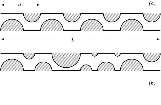
FIG. 1.: Periodic (a) and aperiodic (b) chains of chaotic billiards. The chain length is denoted by $L$, $a$ is the size of an individual billiard. Thus $N=L/a$ is the number of units in the chain.

FIG. 2.: Typical discretized band spectra of a periodic chain with $N=16$ unit cells. The energy levels are shown as a function of the Bloch phase $\theta_{n}$ for 10 bands in the case of (a) low, (b) intermediate and (c) high conductance.

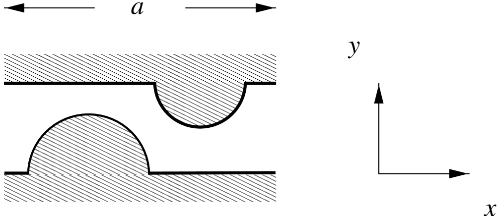
FIG. 3.: Unit cell of the chain of chaotic billiards.

FIG. 4.: $K(\tau)$ for chains of chaotic billiards and different strengths of disorder.

FIG. 5.: The form factor for a quantum graph consisting of N=8 unit cells with $2\times 4$ vertices each. The unit cell is shown in the inset with each dot corresponding to a vertex. The form factors were computed using the lowest 10,000 bands. Each spectral window in Eq. (43) contained 30 bands. The disorder strengths were (top to bottom) $\Delta=0,\,0.02,\,0.05,\,0.1,\,0.5$. The smooth curve represents the theoretical prediction without disorder.

FIG. 6.: Reduction of the form factor due to disorder for various values of the disorder strength $\Delta=0.01,\,0.02,\,0.05,\,0.1,\,0.2,\,0.5$ (bottom to top) compared to the prediction of Eq. (19).

FIG. 7.: The form factor (see Eq. 23) for the unperturbed system with lenght $N=64$ (dots), the corresponding smoothed data (points) and the approximation Eq. 26 and 27 (lines). For $\tau<1/\pi$ the first term in the Bessel function expansion dominates the form factor. After averaged over $1/\pi N$ in $\tau$, the smoothed data fit to the theoretical function (29). For $\tau>1/\pi$ the soothed form factor converges to $\gamma\approx 2$. Here the average is taken over a window of $1/\pi$ in $\tau$.

FIG. 8.: Comparison between the form factor averaged for $1000$ samples ($\sigma=0.008,N=32$) and our perturbative expression. Both of them are smoothed over a $0.5$ window in $\tau$. Points are from the numerical calculation, the solid line is the perturbativ formula of Eq. (35)

FIG. 9.: The universal function $A(\alpha)$.

FIG. 10.: Large–$\tau$ behaviour of the form factor for a periodic and a weakly disordered ($\Delta=0.01$) quantum graph (upper and lower solid lines, respectively) with $N=8$ unit cells. The horizontal dashed lines represent the asymptotic values $K(\tau)=2-2/N$ and $K(\tau)=1$. The heavy dashed lines show $\langle K(\tau,\sigma)\rangle_{\tau}$ according to Eq. (49). The parameter $\sigma$ entering Eq. (49) via Eq. (36) has been determined by adjusting the the location of the minimum of the function $A(2\alpha)$ to the minimum observed in the numerical data.

REFERENCES

- [1] T. Dittrich, B. Mehlig, H. Schanz, and U. Smilansky, Chaos, Solitons & Fractals 8, 1205 (1997). Phys. Rev. E 57, 359 (1998).
- [2] B. D. Simons and B. L. Altshuler, Phys. Rev. Lett. 70, 4063 (1993). N. Taniguchi and B. L. Altshuler, Phys. Rev. Lett. 71, 4031 (1993).
- [3] B. I. Shklovskii, B. Shapiro, B. R. Sears, P. Lambrianidis, H. B. Shore, Phys. Rev. B 47, 11487 (1993).
- [4] M. V. Berry, Proc. R. Soc. A 400, 229 (1985).
- [5] M. C. Gutzwiller, J. Math. Phys. 12, 343 (1971).
-
[6]
T. Dittrich and U. Smilansky, Nonlinearity 4, 85 (1991).
N. Argaman, Y. Imry, and U. Smilansky, Phys. Rev. B 47, 4440 (1993). - [7] T. Dittrich, E. Doron, and U. Smilansky, J. Phys. A 27, 79 (1994).
- [8] T. Dittrich, Phys. Rep. 271, 267 (1996).
- [9] J. H. Hannay and A. M. Ozorio de Almeida, J. Phys. A 17, 3429 (1984).
- [10] T. Kottos and U. Smilansky, Phys. Rev. Lett. 79 (1997) 4794-4797.
- [11] P. Lloyd, J. Phys. C2, 1717 (1969)
- [12] J. Cserti, G. Szálka and G. Vattay, cond-mat/9710264 .
- [13] M. L. Mehta, Random Matrices and the Statistical Theory of Energy Levels, Academic Press, New York and London (1967)
- [14] Chaos in Quantum Physics, in NATO ASI Les Houches series Eds. M.-J. Giannoni, A. Voros and J. Zinn-Justin, North-Holland (1991)
- [15] E.A.Hansen, A Table of Series and Products, (5.22.10) , Prentice-Hall (1975)