Polymer Adsorption on Fractal Walls

Abstract

Polymer adsorption on fractally rough walls of varying dimensionality is studied by renormalization group methods on hierarchical lattices. Exact results are obtained for deterministic walls. The adsorption transition is found continuous for low dimension $d_{w}$ of the adsorbing wall and the corresponding crossover exponent $\phi$ monotonically increases with $d_{w}$, eventually overcoming previously conjectured bounds. For $d_{w}$ exceeding a threshold value $d_{w}^{*}$, $\phi$ becomes 1 and the transition turns first–order. $d_{w}^{*}>d_{saw}$, the fractal dimension of the polymer in the bulk. An accurate numerical approach to the same problem with random walls gives evidence of the same scenario.

1 Introduction

The adsorption on an attracting impenetrable wall is perhaps the most elementary transition involving a single interacting polymer in solution [1]. High dilution in a good solvent is the realistic condition for which this problem can be directly relevant. The fundamental character and the obvious relation with more complex applications, like colloid stabilization or surface protection [2], attracted on polymer adsorption a great deal of attention in recent years, and much information is presently available on this problem. It is now well understood that this transition can be interpreted as a surface critical phenomenon [1, 3]: at the adsorption temperature $T_{a}$ the conformational statistics of the polymer shows a multicritical behavior with peculiar geometric features and with crossovers to the high-$T$ desorbed and the low-$T$ adsorbed regimes. For a chain with $N$ monomers at $T_{a}$ the average number of adsorbed monomers, $\langle M\rangle$, scales as $\langle M\rangle\propto N^{\phi}$, where $\phi$ ($0<\phi<1$) is the crossover exponent. In the high- and low-$T$ regimes, $\langle M\rangle\propto N^{0}$ and $\langle M\rangle\propto N$, respectively. $\phi$ is known exactly in $2D$ for a polymer in both good [4] and theta [5] solvents, and in $3D$ in theta solvent, in which case logarithmic corrections are present [6]. Further exact results have been obtained for models defined on fractal lattices, like Sierpinski gaskets [7, 8, 9], which are by now recognized as an important context in which to test theoretical ideas concerning polymer statistics.

Most explicit results obtained so far on polymer adsorption refer to cases in which the wall is smooth and flat. In this paper we address the adsorption transition on a fractal substrate. This problem has applicative interest. Indeed, in many processes involving polymers, highly corrugated, irregular walls may be present. In addition there are interesting theoretical implications. A polymer in good solvent is known to possess a self–similar stochastic geometry, with a well defined fractal dimension $d_{saw}$. Once such a polymer is put in contact with a fractal wall, a competition between the two geometries arises. This holds in particular for cases in $2D$ or in hierarchical lattices, for which the wall is topologically one–dimensional like the polymer. As we will see, the above competition leads to a modification of the universal properties of the adsorption transition, or, in more extreme situations, to a drastic and quite unusual suppression of its continuous character. The parameter triggering such modifications is the fractal dimension $d_{w}$ of the wall. This scenario has also analogies with another situation in which competition between two similar scaling geometries has been studied recently. A fluctuating interface between two coexisting phases is self–affine [10]. If it is put in contact with a rough wall of similar geometry, depinning from the wall turns from continuous to first–order as soon as the roughness exponent of the wall exceeds the anisotropy index of interface fluctuations in the bulk [11, 12].

An approach to our problem on Euclidean lattice would meet very serious difficulties. Once assigned a given profile to a fractal wall exerting short range attraction on a self–avoiding chain (SAW), exact enumerations would handle too short chains, unable to feel the fractal corrugations of the wall on a sufficiently wide range of length scales. On the other hand, Monte Carlo simulations meet the serious obstacle that, in the low-$T$ region, sampling over polymer configurations becomes very problematic, due to the highly irregular wall, with valleys and hills at all scales. For these reasons adsorption on fractal walls is certainly one of those phenomena for which the study on simplified, hierarchical lattices is at present the only realistic way to gain an at least qualitative understanding. Two recent works studied adsorption on fractal boundaries of SAW’s within fractal lattices [13, 14]. Most emphasis there was put on the existence of violations of bounds suggested in previous work [7] for $\phi$. It was also realized that fractal lattices with peculiar connectivities at the borders could give rise to an interesting dependence of $\phi$ on the interaction parameters. However, such nonuniversality, met also with flat walls, is specific of the lattices considered, which do not mimic generic situations. Indeed, it is natural to expect universal scaling at the adsorption transition for a given (universal) bulk criticality and a given boundary geometry (no matter whether flat or rough). Changes of $\phi$ should be expected upon varying $d_{w}$. This is indeed the dimension pertaining to the surface critical phenomenon to which adsorption amounts.

Here we study adsorption in three hierarchical lattices leading to renormalization group (RG) recursions of increasing complexity and, supposedly, to results of increasing qualitative value with reference to realistic situations on $2D$ Euclidean lattice.

2 Models and Results

Let us consider first the lattice ${\cal L}_{A}$, whose construction rule is sketched in Figure 1a. Measuring the lattice “linear size” in terms of the number of steps of the shortest path between top and bottom vertices, at any application of the construction rule, this size and the total number of lattice bonds are multiplied by factors 2 and 5, respectively. Thus, ${\cal L}_{A}$ has a fractal dimension $d_{L}=\ln 5/\ln 2=2.322\ldots$ At any level, $n$, in the construction of ${\cal L}_{A}$, allowed polymer configurations correspond to SAW’s between the top and bottom vertices. In a grand canonical formulation, to each step is associated a monomer fugacity $\omega=\exp({\mu}/T)$. An attracting impenetrable wall is modeled as a particular SAW which can not be trespassed by the polymer. The polymer interacts with the wall through an attractive contact potential $-\epsilon$. Thus, SAW steps on the wall acquire an extra fugacity $k=\exp(\epsilon/T)$ ($k\geq 1$).

In the absence of wall, through the $n=0$ lattice there is a unique walk of unit length and the restricted grand partition function for SAW’s joining top to bottom is simply $B_{0}=\omega$. At level $n=1$ there are two pairs of SAW’s of lengths 2 and 3, respectively. The corresponding partition function is $B_{1}=2\omega^{2}+2\omega^{3}=2B_{0}^{2}+2B_{0}^{3}\equiv{\cal B}(B_{0})$. If we denote by $B_{n}$ the SAW partition at level $n$, we can write $B_{n+1}\equiv{\cal B}(B_{n})$ and $\cal B$ can be seen as a generating function of the bulk partition function. The recursion for $B_{n}$ has a repulsive fixed point at $B^{*}=(\sqrt{3}-1)/2=0.366\ldots$ which corresponds to the bulk critical point of SAW’s. Thus $\omega_{c}=B^{*}$ is the SAW critical fugacity. For an $n$-th level lattice the average number of SAW steps is given by $\langle N_{B}\rangle_{n}={{\omega}\over{B_{n}}}\ {{\partial B_{n}}\over{\partial\omega}}$. At $\omega=\omega_{c}$ we have $\langle N_{B}\rangle_{n}=\lambda_{B}^{n}$ with $\lambda_{B}=\left.{{d{\cal B}(B)}\over{dB}}\right|_{B^{*}}=2.268\ldots$ Therefore, taking into account that the lattice size is $L_{n}=2^{n}$, we conclude that critical SAW’s are fractal with dimension $d_{saw}=\ln\lambda_{B}/\ln 2=1.181\ldots$

Now let us consider a wall through ${\cal L}_{A}$. In Figure 1b and 1c we sketch two examples of deterministic rules by which wall geometries with opposite features can be realized. Iteration of the rule sketched in Figure 1b produces a wall whose length is $L_{n}$. Thus, this wall is characterized by a dimension $d_{w}=1$ and we regard it as flat. On the contrary, the rule in Figure 1c produces a fractal wall with dimension $d_{w}=\ln 3/\ln 2=1.585\ldots$ which is also the highest realizable in ${\cal L}_{A}$. Walls with intermediate dimensions can be obtained by using either deterministic, or random sequences of the two rules above at progressing levels of lattice construction. As an example, let us consider a case in which the wall is realized by means of rule 1c and 1b for odd and even $n$, respectively. The resulting wall has a dimension $d_{w}=\ln 6/\ln 4=1.292\ldots$ and is sketched in Figure 1d. For $n=1$ the SAW partition function in the presence of the wall is given by

$$X_{1}=X_{0}^{3}+X_{0}B_{0}\equiv{\cal X}_{2}(B_{0},X_{0})$$ (1)

where $X_{0}=k\omega$ is the partition of the unique SAW in the $n=0$ lattice. At $n=2$ we have

$$X_{2}=X_{1}^{2}+2X_{1}B_{1}^{2}+B_{1}^{2}\equiv{\cal X}_{1}(B_{1},X_{1}).$$ (2)

${\cal X}_{1}$ and ${\cal X}_{2}$ are now the generating functions of the SAW partitions corresponding to rules 1b and 1c, respectively. At any other construction level, the form of the recursions is the same as in Equation (1) or Equation (2) for $n$ even or odd, respectively. Focusing attention on even $n$, if $X_{n}$ denotes the SAW partition at level $n$, we have

$$X_{n+2}={\cal X}_{2}({\cal B}(B_{n}),{\cal X}_{1}(B_{n},X_{n})).$$ (3)

For $B=\omega_{c}$ the bulk recursion is at its repulsive fixed point, while (3) has an attractive fixed point at $X=0.1536\ldots$ and a repulsive one at $X\equiv x_{c}\equiv 0.7249\ldots$ [15] Another attractive fixed point is at $X=\infty$. While the first fixed point controls the SAW ordinary desorbed regime, the second one corresponds to the adsorption critical point which is then located at a wall attraction $k_{c}=x_{c}/\omega_{c}=1.9806\ldots$ The critical exponents can be obtained by linearization of the RG flow around the fixed point $(\omega_{c},x_{c})$. In doing this, together with the recursion (3) we have to consider also $B_{n+2}={\cal B}({\cal B}(B_{n}))$ and the matrix

$${\bf R}\equiv\left(\begin{array}[]{cc}\left.{{\partial B_{n+2}}\over{\partial B_{n}}}\right|_{\omega_{c},x_{c}}&\left.{{\partial B_{n+2}}\over{\partial X_{n}}}\right|_{\omega_{c},x_{c}}\\ \left.{{\partial X_{n+2}}\over{\partial B_{n}}}\right|_{\omega_{c},x_{c}}&\left.{{\partial X_{n+2}}\over{\partial X_{n}}}\right|_{\omega_{c},x_{c}}\end{array}\right)=\left(\begin{array}[]{cc}\lambda_{B}^{2}&0\\ a&\lambda_{1}^{2}\end{array}\right)$$ (4)

with

$$\lambda_{1}=\left[\left.{{\partial X_{n+2}}\over{\partial X_{n}}}\right|_{\omega_{c},x_{c}}\right]^{1/2}=\left[\left.{{\partial{\cal X}_{1}}\over{\partial X_{n}}}\right|_{\omega_{c},x_{c}}\cdot\left.{{\partial{\cal X}_{2}}\over{\partial X_{n}}}\right|_{\omega_{c},x_{c}}\right]^{1/2}=1.7412\ldots$$ (5)

and $a=\left.{{\partial X_{n+2}}\over{\partial B_{n}}}\right|_{\omega_{c},x_{c}}$. If we put $\langle N\rangle_{n}={\omega\over{X_{n}}}{{\partial X_{n}}\over{\partial\omega}}$ and $\langle M\rangle_{n}={k\over{X_{n}}}{{\partial X_{n}}\over{\partial k}}$, at the transition, the average number of steps on the wall grows as $\langle M\rangle_{n}=\lambda_{1}^{n}$. Thus, $\langle M\rangle_{n}\sim L_{n}^{y_{1}}$ with $y_{1}=\ln\lambda_{1}/\ln 2=0.8001\ldots$ On the basis of (4) and (5) one can also write:

$$\langle N\rangle_{n}=\lambda_{1}^{n}+a\lambda_{1}^{2}\ {{\lambda_{B}^{n-2}-\lambda_{1}^{n-2}}\over{\lambda_{B}^{2}-\lambda_{1}^{2}}}$$ (6)

This relation shows that, as long as $\lambda_{1}\leq\lambda_{B}$, in the limit of large $n$, $\langle N\rangle_{n}$ scales as $\lambda_{B}^{n}$. In other terms $\langle N\rangle_{n}\sim L_{n}^{y}$ with $y=y_{B}$. On the other hand, if $\lambda_{1}>\lambda_{B}$, $\langle N\rangle_{n}\sim\lambda_{1}^{n}$ and $y=\ln\lambda_{1}/\ln 2=y_{1}$. In this latter case, which, as we will see below, is never realized for ${\cal L}_{A}$, one must find $y_{1}=d_{w}$ because $\langle M\rangle_{n}\sim\langle N\rangle_{n}$, which again means $\phi=1$. At the adsorption fixed point of (3) ($k=k_{c}$), $\lambda_{1}<\lambda_{B}$: thus, there, the SAW length in the presence of wall scales as in the bulk without wall. The previous results allow to write $\langle M\rangle_{n}\sim\langle N\rangle_{n}^{\phi}$ with $\phi=y_{1}/y_{B}=0.6773\ldots$

For any $k>k_{c}$ the SAW’s are adsorbed on the wall and the scalings of both $\langle M\rangle_{n}$ and $\langle N\rangle_{n}$ are controlled by a fixed point at infinity. In this case both quantities are proportional to $L_{n}^{d_{w}}$. On the other hand, for $k<k_{c}$, we are in the normal regime in which $\langle N\rangle_{n}\sim L_{n}^{y_{B}}$. For SAW’s on Euclidean lattice, in this last regime, $\langle M\rangle_{n}$ saturates to a constant value. To the contrary, the analysis of recursion (3) around $X=0.1536\ldots$ shows that $\langle M\rangle_{n}\sim L_{n}^{-1.0844\ldots}$. This unphysical behavior is due to the pathological increase of coordination with $n\to\infty$ typical of hierarchical lattices. The above discussion can of course be adapted to the case of odd $n$ levels, with the same scaling results.

The method just illustrated can be easily generalized to fractal walls with a whole range of $d_{w}$. In fact, adsorption on walls with different dimensions can be obtained by simply changing the form of the recursion. In general, in place of (3), we can have $p$ and $q$ nested applications of the generating functions ${\cal X}_{1}$ and ${\cal X}_{2}$, respectively. For example, for $p=2$ and $q=3$ we could have

$$X_{n+p+q}=$$

$${\cal X}_{1}({\cal B}({\cal B}({\cal B}({\cal B}(B_{n})))),{\cal X}_{2}({\cal B}({\cal B}({\cal B}(B_{n}))),{\cal X}_{2}({\cal B}({\cal B}(B_{n})),{\cal X}_{1}({\cal B}(B_{n}),{\cal X}_{2}(B_{n},X_{n})))))$$ (7)

which corresponds to applying successively ${\cal X}_{2}$, ${\cal X}_{1}$, ${\cal X}_{2}$, ${\cal X}_{2}$, and ${\cal X}_{1}$. The corresponding wall has $d_{w}={{(p\ln 2+q\ln 3)}\over{(p+q)\ln 2}}$. For given $p$ and $q$, we could generate many different recursions by changing the order in which ${\cal X}_{1}$ and ${\cal X}_{2}$ are applied. While this order influences the position of the adsorption transition point, the corresponding critical exponents are only functions of the wall dimension. This property follows from the circumstance that by construction the different RG recursions are diffeomorphically related. This is the mechanism by which $d_{w}$ alone, and no other features of the wall, determines the critical exponents of the transition. In these more general conditions we find

$$\lambda_{1}=\left[\left.{{\partial X_{n+p+q}}\over{\partial X_{n}}}\right|_{\omega_{c},x_{c}}\right]^{1/(p+q)}=\left[\left(\left.{{\partial{\cal X}_{1}}\over{\partial X}}\right|_{\omega_{c},x_{c}}\right)^{p}\cdot\left(\left.{{\partial{\cal X}_{2}}\over{\partial X}}\right|_{\omega_{c},x_{c}}\right)^{q}\right]^{1/(p+q)}$$ (8)

where $x_{c}$ has to be calculated for the specific form of $X_{n+p+q}$. As already mentioned, $d_{w}$ can be varied between $1$ and $\ln 3/\ln 2$ in ${\cal L}_{A}$. The lower limit corresponds to $p=1$ and $q=0$. In this case we have $k_{c}=1$ and $\lambda_{1}=1$ which implies $\phi=0$. In fact, for this case of “flat” boundary, the adsorption transition fixed point merges with the desorbed regime fixed point and becomes marginally unstable. This is a peculiar feature due to the relatively too simple structure of ${\cal L}_{A}$. On the other hand, the upper limit corresponds to $p=0$ and $q=1$ for which one has $k_{c}=\sqrt{3+\sqrt{3}}$ and $\lambda_{1}\equiv\lambda_{B}$. In this case we have exactly $\phi=1$. For intermediate wall dimensions, $\phi$ is a monotonic increasing function of $d_{w}$. A summary of our results for ${\cal L}_{A}$ is reported in Table 1.

$\phi<1$ implies continuity of the adsorption transition. On the contrary, for $\phi=1$, at the transition $\langle M\rangle_{n}\propto\langle N\rangle_{n}$, as for an adsorbed polymer. In fact $\lambda_{1}\geq\lambda_{B}$ implies a discontinuity of $\lim_{n\to\infty}[\langle M\rangle_{n}/\langle N\rangle_{n}]$ at the adsorption point, i.e. a first–order transition. This discontinuity, found only for $d_{w}=\ln 3/\ln 2$ in ${\cal L}_{A}$, anticipates a more general result, valid for the other lattices we considered: we find below that a sufficiently high $d_{w}$ can drive polymer adsorption first–order. For ${\cal L}_{A}$ the threshold condition for discontinuous adsorption occurs precisely when $d_{w}$ is at its maximum possible value. In general we will denote by $d^{*}_{w}$ the value of $d_{w}$ above which $\phi=1$.

To show that the scenario described above is not just peculiar of ${\cal L}_{A}$ and to investigate further the change of transition order, we considered SAW adsorption on fractal walls also with ${\cal L}_{B}$ and ${\cal L}_{C}$, sketched in Figures 2a and 3a, respectively. ${\cal L}_{B}$ has a diamond structure similar to that of ${\cal L}_{A}$, but with a higher ramification and $d_{L}=3$. The bulk SAW partition function obeys the recursion $B_{n+1}=3B_{n}^{2}+4B_{n}^{3}+2B_{n}^{4}$ with $\omega_{c}=B^{*}=0.2441\ldots$ and $d_{saw}=1.1995\ldots$ In Figure 2b and 2c we report two construction rules generating walls with dimensions $d_{w}^{(1)}=1$ and $d_{w}^{(2)}=2$, respectively. The corresponding generating functions are:

$${\cal X}_{1}(X,B) \equiv X^{2}+2XB^{2}+B^{2}$$ (9)

$${\cal X}_{2}(X,B) \equiv XB+X^{2}B+X^{4}.$$ (10)

For fractal walls obtained by suitably alternating the two rules, Table 2 shows again that $\phi$ monotonically increases with $d_{w}$. However, now for any $d_{w}>1.67$ we have $\phi=1$. Thus, when $d_{w}>d_{w}^{*}\simeq 1.67$ adsorption becomes discontinuous.

Finally, we consider ${\cal L}_{C}$ for which $d_{L}=\ln 12/\ln 4=1.792\ldots$ [16]. The bulk recursion is now $B_{n+1}=6B_{n}^{4}+4B_{n}^{6}+2B_{n}^{8}$ with critical fixed point at $\omega_{c}=B^{*}=0.5175\ldots$ and $d_{saw}=1.0649\ldots$ Unfortunately, neither $\omega_{c}$, nor $d_{saw}$ are too close to the values appropriate for $2D$ square lattice, $0.378\ldots$ and 4/3 [17, 3], respectively. This occurs in spite of the fact that ${\cal L}_{C}$ seems to mimic well the square lattice structure at local level. ${\cal L}_{C}$ offers more possibilities of wall construction rules. In Figures 3b, 3c and 3d we show three examples with respective generating functions

$${\cal X}_{1}(X,B) \equiv 2B^{4}+X^{4}+2X^{2}B^{2}+2X^{2}B^{4}$$ (11)

$${\cal X}_{2}(X,B) \equiv XB^{3}+X^{2}B^{4}+X^{5}B^{3}+X^{2}B^{2}+X^{3}B+X^{6}$$ (12)

$${\cal X}_{3}(X,B) \equiv X^{3}B+X^{5}B+X^{8}$$ (13)

The corresponding walls have $d_{w}^{(1)}=1$, $d_{w}^{(2)}=\ln 6/\ln 4=1.292\ldots$ and $d_{w}^{(3)}=\ln 8/\ln 4=1.5$. Results for ${\cal L}_{C}$ are reported in Table 3. For $d_{w}=1$ adsorption is continuous and $\phi=0.5437\ldots$ is not too far from 1/2, the $\phi$ value for SAW adsorption on a smooth wall in $2D$ [4]. For increasing $d_{w}$, $\phi$ monotonically increases and reaches a unit value at $d_{w}=d_{w}^{*}\simeq 1.4$. For $d_{w}>d_{w}^{*}$, $\phi=1$ and the transition is always first–order. Note that the first–order transitions found for $d_{w}>d_{w}^{*}$ in Tables 2 and 3 correspond to $\lambda_{1}>\lambda_{B}$. From Tables 1, 2 and 3 we also learn that, upon increasing $d_{w}$, $k_{c}$ increases, as a rule, up to small fluctuations caused by our peculiar recipe for varying $d_{w}$. This indicates that increasing roughness makes adsorption more difficult.

Our results suggest an interesting scenario for the adsorption transition on fractal walls in more realistic models. First of all, for a continuous adsorption transition, $\phi$ is an increasing function of the wall dimension $d_{w}$. Moreover, for high enough $d_{w}$, $\phi$ eventually reaches the value 1, its upper bound marking the onset of first–order adsorption. This fact is in open contrast with the results of Bouchaud and Vannimenus [7] which, on the basis of scaling arguments, suggested the bounds

$$1-{1\over{d_{saw}}}(d_{L}-d_{w})\leq\phi\leq{{d_{w}}\over{d_{L}}}.$$ (14)

We find that $\phi$ does not satisfy (14). Also the lower bound in (14) is manifestly violated for low enough $d_{w}$. Of course, here we deal with a hierarchical lattice, which is not fully adequate to represent consistently all the features of fractal objects. On the other hand, the bounds in (14) were obtained by relying on formal analogies with cases of regular geometry. Similar violations of these bounds were reported previously, for both flat and fractal boundaries [9, 13]. Here we identify in the monotonicity of $\phi$ and in the tendency of the transition to turn first–order as $d_{w}$ increases the physical reasons for the upper bound violation. In the investigation of Ref. [14] first–order adsorption was found for a particular choice of lattice and fractal boundary among the many considered. A posteriori, we can understand that result as due to the fact that such choice determines a rather high $d_{w}$ relative to $d_{saw}$.

We obtained also results for random fractal walls. Unlike the case of deterministic walls above, this problem cannot be solved exactly, even on hierarchical lattices. However, quantities like $\overline{\langle M\rangle}_{n}$ and $\overline{\langle N\rangle}_{n}$, which now have to be averaged also over wall randomness (overbar represents this average), can be calculated quite accurately also for very large system sizes by a Monte Carlo approach [11, 12, 18]. We performed these calculations for ${\cal L}_{C}$ with walls obtained by random combined applications of the rules in Figure 3c and 3d. At any level of lattice construction, we choose whether the wall is realized by rule $3c$ or $3d$ with probabilities $1-\Delta$ and $\Delta$ ($\Delta<1$), respectively. Of course, this determines which of the two generating functions, ${\cal X}_{2}$ (Equation (12)) and ${\cal X}_{3}$ (Equation (13)), has to be used in order to calculate $X_{n+1}$ in terms of $X_{n}$. For $0<\Delta<1$ the wall has, on average, a fractal dimension $d_{w}=\ln(6+2\Delta)/\ln 4$. $X_{n}$ becomes now a random variable and we must consider its probability distribution. Of course, we can only produce a finite sampling of this distribution, by proceeding as follows. From a large set (up to $4\cdot 10^{5}$ elements) $\{X_{n}\}$ of $n$–th level partition values we generate each element of the new sample $\{X_{n+1}\}$ by choosing first, with the appropriate probabilities, between rules (12) and (13); then from $\{X_{n}\}$ are extracted at random the elements needed as entries into (12) or (13), and an element $X_{n+1}$ of the new sample is computed as a function of them and of $B_{n}$. Using some numerical tricks to control the possible rapid divergence of the partition functions near the transition, we could iterate this procedure up to $n=30\div 35$.

By analyzing the scaling of $\overline{\langle M\rangle}_{n}$ and $\overline{\langle N\rangle}_{n}$ at the transition point (which now has to be numerically determined) as a function of $L_{n}$, we could estimate $\phi$ for different $\Delta$’s as reported in Figure 4. Even if the relative poorness of the samplings causes appreciable uncertainty in the $\phi$ determinations (Figure 4), we see that this exponent stabilizes for $\Delta>1/2$ to a value compatible with the upper limit $\phi=1$. The results are consistent with the scenario for deterministic walls. In particular, $\Delta=1/2$ corresponds to $d_{w}=1.404$, extremely close to $d_{w}^{*}\simeq 1.4$ applying in that case. All this suggests that first–order adsorption should be expected also with random fractal walls, with the same threshold $d_{w}^{*}$ as in the deterministic case.

3 Conclusions

Our most remarkable result here is the roughness induced change into first–order of the adsorption transition. Without any other changes in the polymer–wall interactions, high enough $d_{w}$ make the adsorption transition discontinuous. This is found in all lattices considered, although marginally in ${\cal L}_{A}$. The change in the nature of the transition takes place for $d_{w}$ definitely larger than $d_{saw}$. In spite of the qualitative value of our model calculations, we can hope that similar properties could hold in realistic situations, in both $2D$ and $3D$.

The change into first-order of the adsorption transition should be imputed to the fact that, upon increasing $d_{w}$, the drop in entropy associated to a localization of the polymer near the wall, increases with $d_{w}$. Even if it is not easy to give a precise meaning to the notion of distance of a polymer from a fractal substrate, at qualitative level we can argue that the entropic repulsion effect due to localization [19], should create a free energy barrier, whose height and (long) range certainly increase as $d_{w}$ gets larger. The rougher the surface, the more it limits the configurations of the confined polymer. Thus, we can think $d_{w}^{*}$ as the maximum dimension for which “tunneling” of the polymer can still occur continuously from the attractive free energy well at small distance to the unbound state at infinite distance across the barrier. For $d_{w}>d_{w}^{*}$, the “tunneling” becomes discontinuous because of the too large barrier (this means that the SAW, right at the desorption point, is not delocalized yet, as occurs in continuum adsorption).

A mechanism like the qualitative one outlined above has been demonstrated and precisely described for the phenomenon of wetting of self–affine rough substrates in $2D$, which has some analogies with our adsorption [12]. Indeed, in that case one finds that a fluctuating interface depinns discontinuously from a rough substrate as soon as the roughness of the latter (measured by its self–affinity exponent $\zeta_{w}$) exceed $\zeta_{0}$, the exponent specifying the intrinsic roughness of the interface in the bulk [11, 12]. The coincidence of the threshold roughness with $\zeta_{0}$ (which by analogy, would suggest $d_{w}=d_{w}^{*}$ here) is a peculiar feature of the interfacial problem in $2D$. Indeed, for that problem, the possibility of a path–integral description in $1+1$ dimensions allows to establish a correspondence with the $1D$ quantum tunneling of a particle across a long range repulsive potential barrier. It turns then out that a roughness $\zeta_{w}=\zeta_{0}=1/2$ determines a decay of this potential right at the threshold for discontinuous tunneling [12]. Our results here show that fractal wall roughness leaves room for a continuous polymer adsorption also when $d_{w}>d_{saw}$.

References

Table 1: SAW adsorption on deterministic fractal walls in ${\cal L}_{A}$. Wall rules are applied in the reported order.

• $d_{L}=\ln 5/\ln 2=2.3219$, $\omega_{c}=0.3660$, $d_{saw}=1.1814$
  	$d_{w}$	$k_{c}$	$\phi$
  ${\cal X}_{1}$	1	1	0
  ${\cal X}_{2},{\cal X}_{1},{\cal X}_{1},{\cal X}_{1},{\cal X}_{1},{\cal X}_{1}$	1.0975	1.7398	0.3856
  ${\cal X}_{2},{\cal X}_{1},{\cal X}_{1},{\cal X}_{1},{\cal X}_{1}$	1.1170	1.7725	0.4230
  ${\cal X}_{2},{\cal X}_{1},{\cal X}_{1},{\cal X}_{1}$	1.1462	1.8165	0.4736
  ${\cal X}_{2},{\cal X}_{1},{\cal X}_{1}$	1.1950	1.8798	0.5483
  ${\cal X}_{2},{\cal X}_{2},{\cal X}_{1},{\cal X}_{1},{\cal X}_{1}$	1.2340	2.0267	0.5957
  ${\cal X}_{2},{\cal X}_{1}$	1.2925	1.9806	0.6773
  ${\cal X}_{2},{\cal X}_{2},{\cal X}_{1}$	1.3900	2.1051	0.7904
  ${\cal X}_{2}$	1.5850	2.1753	1a

• $\lambda_{1}=\lambda_{B}$

Table 2: SAW adsorption on deterministic fractal walls in ${\cal L}_{B}$.

• $d_{L}=3$, $\omega_{c}=0.2441$, $d_{saw}=1.1995$
  	$d_{w}$	$k_{c}$	$\phi$
  ${\cal X}_{1}$	1	3.3049	0.6613
  ${\cal X}_{2},{\cal X}_{1},{\cal X}_{1},{\cal X}_{1}$	5/4	3.3476	0.8124
  ${\cal X}_{2},{\cal X}_{1},{\cal X}_{1}$	4/3	3.3500	0.8628
  ${\cal X}_{2},{\cal X}_{1}$	3/2	3.3549	0.9637
  ${\cal X}_{2},{\cal X}_{2},{\cal X}_{1}$	5/3	3.3629	1a
  ${\cal X}_{2},{\cal X}_{2},{\cal X}_{2},{\cal X}_{1}$	7/4	3.3652	1a
  ${\cal X}_{2}$	2	3.3663	1a

• $\lambda_{1}>\lambda_{B}$

Table 3: SAW adsorption on deterministic fractal walls in ${\cal L}_{C}$.

• $d_{L}=\ln 12/\ln 4=1.7925$, $\omega_{c}=0.5175$, $d_{saw}=1.0649$
  	$d_{w}$	$k_{c}$	$\phi$
  ${\cal X}_{1}$	1	1.3279	0.5437
  ${\cal X}_{2}$	1.2925	1.4715	0.8140
  ${\cal X}_{3},{\cal X}_{2}$	1.3962	1.6287	0.9741
  ${\cal X}_{3},{\cal X}_{3},{\cal X}_{2}$	1.4308	1.6514	1a
  ${\cal X}_{3}$	1.5	1.6565	1a

• $\lambda_{1}>\lambda_{B}$

Figure 1: $a$ Construction rule of ${\cal L}_{A}$. The length of the diagonal step is different from the other lattice steps only for drawing convenience. $b$–$d$ Construction rules of deterministic fractal walls (heavy lines) in ${\cal L}_{A}$. The allowed polymer configurations develop to the right of the walls.

Figure 2: $a$ Construction rule of ${\cal L}_{B}$. $b$–$c$ Construction rules of deterministic fractal walls (heavy lines) in ${\cal L}_{B}$.

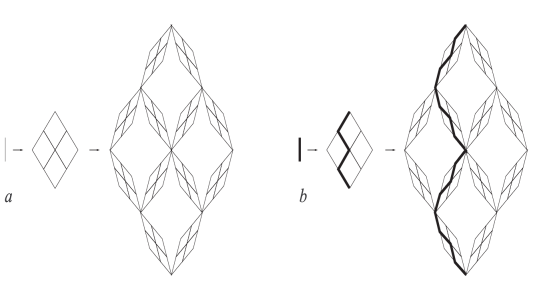
Figure 3: $a$ Construction rule of ${\cal L}_{C}$. $b$–$d$ Construction rules of deterministic fractal walls (heavy lines) in ${\cal L}_{C}$.

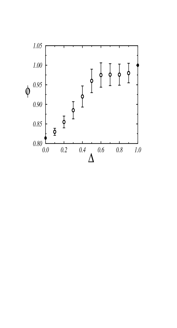
Figure 4: $\phi$ as a function of $\Delta$ for SAW adsorption on random fractal walls in ${\cal L}_{C}$. $\phi$ values at $\Delta=0$ and $\Delta=1$ (closed circles) are exact.

References

- [1] K. De Bell and T. Lookman, Rev. Mod. Phys. 65, 87 (1993).
- [2] D. Nopper, “Polymer Stabilization of Colloidal Dispersions”, (Academic Press, New York, 1983).
- [3] C. Vanderzande, “Lattice Models of Polymers”, (Cambridge University Press, 1998).
- [4] T. W. Burkhardt, E. Eisenriegler and I. Guim, Nucl. Phys. B 316, 559 (1989).
- [5] C. Vanderzande, A. L. Stella and F. Seno, Phys. Rev. Lett. 67, 2757 (1991).
- [6] H. W. Diehl and E. Eisenriegler, Europhys. Lett. 4, 709 (1987).
- [7] E. Bouchaud and J. Vannimenus, J. Physique (Paris) 50, 2931 (1989).
- [8] S. Kumar and Y. Singh, Phys. Rev. E 48, 734 (1993).
- [9] I. Zivić, S. Milosević and H. E. Stanley, Phys. Rev. E 49, 636 (1994).
- [10] G. Forgacs, R. Lipowsky and Th.M. Nieuwenhuizen, in “Phase Transitions and Critical Phenomena”, by C. Domb and J.L. Lebowitz, Vol. 14, (Academic Press, London, 1991).
- [11] G. Giugliarelli and A.L. Stella, Phys. Rev. E 53, 5035 (1996)
- [12] A. L. Stella and G. Sartoni, Phys. Rev. E 58, 2979 (1998).
- [13] V. Miljković, S. Milosević and I. Zivić, Phys. Rev. E 52, 6314 (1995).
- [14] S. Milosević, I. Zivić and V. Miljković, Phys. Rev. E 55, 5671 (1997).
- [15] Fixed points and other numerical results were obtained with MATHEMATICA.
- [16] This lattice and have been used for studying SAW’s in random environment by P. Le Doussal and J. Machta, J. Stat. Phys. 64, 541 (1991).
- [17] B. Nienhuis, Phys. Rev. Lett. 49, 1062 (1982).
- [18] A. Sartori, Tesi di Laurea, University of Padova, (1997).
- [19] P.–G. De Gennes, “Scaling Concepts in Polymer Physics”, (Cornell University Press, Ithaca and London, 1979).
-
, , 1 1 0 1.0975 1.7398 0.3856 1.1170 1.7725 0.4230 1.1462 1.8165 0.4736 1.1950 1.8798 0.5483 1.2340 2.0267 0.5957 1.2925 1.9806 0.6773 1.3900 2.1051 0.7904 1.5850 2.1753 1a -
a
-
, , 1 3.3049 0.6613 5/4 3.3476 0.8124 4/3 3.3500 0.8628 3/2 3.3549 0.9637 5/3 3.3629 1a 7/4 3.3652 1a 2 3.3663 1a -
a
-
, , 1 1.3279 0.5437 1.2925 1.4715 0.8140 1.3962 1.6287 0.9741 1.4308 1.6514 1a 1.5 1.6565 1a -
a