Sine-Gordon low-energy effective theory for Copper Benzoate

Abstract

Specific heat data for the quasi one dimensional quantum magnet Copper Benzoate (${\rm Cu(C_{6}D_{5}COO)_{2}\cdot 3D_{2}O}$) is analyzed in the framework of an effective low-energy description in terms of a Sine-Gordon theory.

PACS: 74.65.+n, 75.10. Jm, 75.25.+z

I Introduction

Quasi one dimensional quantum magnets have been a focus of intense theoretical and experimental interest for a long time. Most of the work is based on and centers around the spin-$1/2$ Heisenberg model [1].

Starting with Bethe’s seminal work [2] a host of exact results have been obtained for ground state properties [3], magnetic susceptibility [4], thermodynamics [5, 6], excitation spectrum [7, 8] and correlation functions [9, 10, 11, 12]. From the point of view of standard spin wave theory, which is highly successful for “three dimensional” materials, the findings of the these investigations were rather unusual. Over the last thirty years a number of anisotropic materials have been found that constitute excellent realizations of the one dimensional Heisenberg model [13], e.g. ${\rm KCuF_{3}}$, ${\rm Sr_{2}CuO_{3}}$, ${\rm Cs_{2}CuCl_{4}}$ or CuPzN, and many theoretical predictions have been confirmed experimentally. One main focus of attention was the spectrum, which comprises of an incoherent (two particle) scattering continuum of elementary excitations, the so-called spinons [7]. These can be visualized in terms of ferromagnetic “domain walls” and are strikingly different from the usual spin waves. In particular spinons are believed to have fractional (semionic) exclusion statistics [14]. The low-energy effective theory of the spin-$1/2$ chain is simply a free massless boson [9, 15, 16]

$${\cal L}=\frac{1}{2}\left(\partial_{\mu}\Phi\right)^{2}\ .$$ (1)

It has been known for some time that Copper Benzoate is another realization of a quasi-1D $S=1/2$ Heisenberg antiferromagnet [17]. However, its response to a magnetic field has been found to be unusual [18]: structural anisotropy leads to to generation of small staggered fields in and perpendicular to the direction of the applied field. Early specific heat measurements [19] showed behaviour incompatible with theoretical results for a simple Heisenberg chain.

In a series of recent experiments [20, 21] the behaviour of Copper Benzoate in a magnetic field was investigated in great detail. Neutron scattering experiments [21] established the existence of field-dependent incommensurate low energy modes. The incommensurability was found to be consistent with the one predicted by the exact solution of the Heisenberg model in a magnetic field. However, the system exhibited an unexpected excitation gap induced by the applied field. As no evidence for ordering was found in the experiments down to temperatures of $0.1-0.3K$ the interchain coupling in Copper Benzoate supposedly is very small (the exchange is approximately 18K). We therefore will neglect it in the present work.

In [22] it was proposed that Copper Benzoate is described by the Hamiltonian

$$H_{\rm CuB}=\sum_{i}J\vec{S}_{i}\cdot\vec{S}_{i+1}-{\tt g}\mu_{B}HS_{i}^{z}+\mu_{B}h(-1)^{i}S^{x}_{i}\ ,$$ (2)

where $H\gg h$, ${\tt g}$ is the effective Landé g-factor and $J=1.57\ {\rm meV}$ [20]. Here the induced staggered field $h$ is a function of the known (staggered) $g$-tensor [18] and the Dzyaloshinskii-Moriya (DM) interaction in Copper Benzoate, for which unfortunately only scant information is available. If direction and magnitude of the DM interaction are given, $h$ is calculated as follows [22]. The $g$-tensor in the $a^{\prime\prime},b,c^{\prime\prime}$ basis (these denote the three principal axes of the exchange interaction [23]) is given by [18]

$$g=\left(\begin{array}[]{ccc}2.115&\pm 0.0190&0.0906\\ \pm 0.0190&2.059&\pm 0.0495\\ 0.0906&\pm 0.0495&2.316\end{array}\right).$$ (3)

The $\pm$ correspond to the two inequivalent sites and indicate that application of a uniform field induces a staggered one. The corresponding contribution to the Hamitonian is

$${\cal H}_{\rm magn}=g_{ab}\ \mu_{B}\ H_{a}\ S^{b}\ .$$ (4)

The staggered DM interaction is

$${\cal H}_{\rm DM} = \sum_{j}(-1)^{j}\ \vec{D}\cdot(\vec{S}_{j}\times\vec{S}_{j+1})\,$$ (5)

where $|\vec{D}|\ll J$ and the direction of $\vec{D}$ is thought to be close to the $a^{\prime\prime}$ axis. The DM interaction is eliminated by a rotation in spin space around the $\vec{D}$-axis by an angle $\alpha=\pm(\arctan D/J)/2$ on even/odd sites. This induces a very small exchange anisotropy which is negligible, and a staggered field

$${\cal H}_{\rm OA}=\frac{g}{2}\mu_{B}(\vec{H}\times\vec{D}/J)\cdot\sum_{j}(-1)^{j}\vec{S}_{j}\ ,$$ (6)

where we used that $|\vec{D}|/J\ll 1$. Combining the two contributions (6) and (4) we obtain the total induced staggered field. For example, a uniform field applied along the $a^{\prime\prime}$ axis induces a staggered field $h$ along the b axis of magnitude $(0.019-2.115D_{c}/2J)H$.

The low energy effective theory of (2) is obtained by abelian bosonization and is given by a Sine-Gordon model with Lagrangian density [22]

$${\cal L}=\frac{1}{2}(\partial_{\mu}\Phi)^{2}+\lambda(h)\cos(\beta\ \Theta)\ .$$ (7)

Here $\Theta$ is the dual field and the coupling $\beta$ depends on the value of the applied uniform field. The coefficient $\lambda(h)$ can at present not be calculated exactly. The reason is that the amplitudes of the bosonized expressions of lattice spin operators for $H>0$ are not known (in the absence of a magnetic field they have been determined very recently in [16, 24, 25]). For later convenience we define the coupling

$$\xi=\frac{\beta^{2}}{8\pi-\beta^{2}}\ .$$ (8)

The Sine-Gordon theory (7), for all its apparent simplicity, has fascinated physicists for decades. It is of interest as an integrable classical nonlinear differential equation featuring soliton solutions. On the quantum level it has been one of the cornerstones of nonperturbative quantum field theory with many exciting features such as quantum solitons, topological charge or regularization dependence in the nonperturbative regime [26]. Most importantly the quantum Sine-Gordon model is exactly solvable [27] and many physically important quantities can be calculated. In particular, the spectrum is known to consist of a soliton-antisoliton doublet of mass $M$ and their bound states which are called “breathers”.

The soliton mass gap $M$ can in principle be calculated exactly [28] in terms of $\beta$ and $\lambda$ for a given short-distance normalization of correlation functions. However, $\lambda$ is known only for the case of vanishing uniform field $H=0$ (see above). A simple analysis based on the results of [28, 16, 25] yields for this case (i.e. one takes to staggered field into account, but bosonizes at $H=0$)

$$M/J \approx \frac{2\Gamma(1/6)}{\sqrt{\pi}\Gamma(2/3)}\left[\pi\frac{\Gamma(3/4)}{\Gamma(1/4)}\sqrt{\frac{\pi}{4(2\pi)^{3/2}}}\right]^{2/3}\left(\frac{h}{J}\right)^{2/3}$$ (9)

$$\approx 1.8\left(\frac{h}{J}\right)^{2/3}\ ,$$ (10)

where we have neglected logarithmic corrections. This is in good agreement with the numerical analysis of the lattice Hamiltonian (2) for $H=0$, which gives [22]

$$M/J\approx 1.85\left(\frac{h}{J}\right)^{2/3}\bigg{|}\log\frac{h}{J}\bigg{|}^{1/6}\ .$$ (11)

In addition to soliton and antisoliton there are $[\frac{1}{\xi}]$ (here $[\ ]$ is the integer part) breathers with masses

$$M_{n}=2M\ \sin n\pi\xi/2\ ;\ n=1,\ldots,\left[1/\xi\right].$$ (12)

The mass spectrum as a function of magnetic field for Copper Benzoate was explicitly determined in [29].

Exact predictions of the low-energy effective theory (7) for the spectrum [22] and the dynamical structure factor [29] were found to be consistent with Neutron scattering experiments for applied fields along the b-axis. It is interesting to note that the Sine-Gordon solitons and breathers are fundamentally different from the spinons of the spin-$1/2$ chain.

In [21] precise measurements of the low-temperature specific heat were presented and analyzed in terms of several noninteracting one-dimensional bosons of the same mass. On the other hand, the spectrum of the Sine-Gordon model in the relevant region of couplings features five interacting modes with different masses [29] (soliton, antisoliton and three breathers).

In the present work we analyze the specific heat data of [21] in the framework of the Sine-Gordon theory. A very important input in the low-energy effective Lagrangian (7) are the values of the coupling $\beta$ and the spin velocity $v_{s}$. In a “minimal” model (MM) they are calculated from the exact Bethe Ansatz solution of the Heisenberg XXX chain in an applied magnetic field $H$ [15]. In Appendix A we summarize the corresponding relevant Bethe Ansatz results.

FIG. 1.: Coupling constant $\beta^{2}/2\pi$ in the MM as a function of the applied magnetic field $H\parallel b$ .

FIG. 2.: Spin velocity in the MM as a function of the applied field $H\parallel b$ .

This procedure appears to be reasonable as long as the induced field $h$ is very small so that its effects on $\beta$ and $v_{s}$ are negligible. The results are shown in Figs 1 and 2 respectively. At very high fields $g\mu_{B}H\approx 2J$ we approach the incommensurate-commensurate transition to the saturated ferromagnetic state [30] and the spin velocity thus tends to zero.

An alternative scenario is to consider the spin velocity and/or the coupling $\beta$ as a phenomenological parameters in the Sine-Gordon theory (7). The rationale behind such an approach is that the known presence of the DM interaction as well as possible exchange anisotropies will lead to deviations in the values of these quantities as compared to the MM predictions.

A simple calculation shows that the effect of the DM interaction on $\beta$ and $v_{s}$ is negligible. Adding an exchange anisotropy

$$H_{\rm anis}=-J\Delta\sum_{j}S^{x}_{j}S^{x}_{j+1}\ ,0<\Delta\ll 1$$ (13)

to the Hamiltonian (2) firstly induces a change in the spin velocity entering the effective Lagrangian (7) and secondly generates the second harmonic of the SG interaction, i.e. the effective low-energy theory becomes [31]

$${\cal L}=\frac{1}{2}(\partial_{\mu}\Phi)^{2}+\lambda\cos(\beta\ \Theta)\ +\mu\cos(2\beta\ \Theta)\ .$$ (14)

Here we have assumed that $\Delta$ is much smaller than the magnetic energy scale $g\mu_{B}H$. The coupling $\mu$ mainly depends on $\Delta$ (the second harmonic also gets generated at 1-loop level by the $\cos\beta\Theta$ interaction). In the regime of couplings $\beta$ we are interested in, the second harmonic is a relevant operator (in the RG sense), although it is of course much less relevant than $\cos\beta\Phi$. This means that we can safely neglect the second harmonic, unless $\lambda\ll\mu$ ! We will return to this point below. Physically the effect of (13) is the following: if no uniform field is applied, the system remains critical. The spin velocity and the critical exponents are changed slightly. If a uniform field is applied perpendicular to the direction of the anisotropy, a spectral gap forms, even if no staggered field is generated.

II Sine-Gordon Thermodynamics

The thermodynamics of the Sine-Gordon model is most efficiently studied [32] via the recently developed Thermal Bethe Ansatz approach [33], which circumvents problems associated with solving the infinite number of coupled nonlinear integral equations that emerge in the standard approach based on the string hypothesis [34] (note that the coupling constant $\beta$ in our problem is a continously varying quantity and no truncation to a finite number of coupled equations is possible). It was shown in [32] that the free energy of the Sine-Gordon model can be expressed in terms of the solution of a single nonlinear integral equation for the complex quantity $\varepsilon(\theta)$ (we set the spin velocity to 1 for simplicity)

$$\varepsilon(\theta)=-iM\beta\sinh(\theta+i\eta^{\prime})$$ (15)

$$-\int_{-\infty}^{\infty}d\theta^{\prime}G_{0}(\theta-\theta^{\prime})\ln\left(1+\exp\left[-\varepsilon(\theta^{\prime})\right]\right)$$ (16)

$$+\int_{-\infty}^{\infty}d\theta^{\prime}G_{0}(\theta-\theta^{\prime}+2i\eta^{\prime})\ln\left(1+\exp\left[-\bar{\varepsilon}(\theta^{\prime})\right]\right),$$ (17)

where $\beta=(k_{B}T)^{-1}$, $M$ is the soliton mass and

$$G_{0}(\theta) = \int_{0}^{\infty}\frac{d\omega}{\pi^{2}}\frac{\cos(2\omega\theta/\pi)\sinh(\omega(\xi-1))}{\sinh(\omega\xi)\cosh(\omega)}\ .$$ (18)

The free energy density is given by

$$f(\beta) = -\frac{M}{\beta\pi}\!\Im m\!\int_{-\infty}^{\infty}\!\!\!\!\!\!d\theta\ \sinh(\theta+i\eta^{\prime})\ln\left[1+e^{-\varepsilon(\theta)}\right].$$ (19)

As we are interested in the attractive regime $\gamma<4\pi$ we have

$$0<\eta^{\prime}<\pi\xi/2\ .$$ (20)

Note that the free energy does not depend on the value of $\eta^{\prime}$ as long as it is chosen in the interval (20). The set (17) of two coupled nonlinear integral equations is solved by iteration. For $\beta\to\infty$ the first iterations can be calculated analytically and the corresponding contributions to the free energy are seen to be of the form

$$f(\beta) \sim -\frac{2M}{\beta\pi}\sum_{n=1}^{\infty}\frac{(-1)^{n+1}}{n}K_{1}(nm\beta)$$ (22)

$$-\frac{M_{1}}{\beta\pi}K_{1}(M_{1}\beta)+\ldots\ ,$$

where $M_{1}=2M\sin\frac{\pi\xi}{2}$ is the mass of the first breather and $K_{1}$ is a modified Bessel function. The first term is the contribution of soliton-antisoliton scattering states to the free energy, whereas the second term is the contribution of the first breather. Both terms have the form characteristic of massive relativistic bosons. The contributions of the heavier breathers are found in higher orders of the iterative procedure employed in solving (17). The specific heat is obtained from the free energy

$$C=T\frac{\partial^{2}f(\beta)}{\partial T^{2}}\ .$$ (23)

At low temperatures it is found to be of the form

$$C \sim \sum_{\alpha=1}^{[1/\xi]}\frac{k_{B}}{\sqrt{2\pi}v_{s}}\left[1+\frac{k_{B}T}{M_{\alpha}}+\frac{3}{4}\left(\frac{k_{B}T}{M_{\alpha}}\right)^{2}\right]$$ (25)

$$\times\left(\frac{M_{\alpha}}{k_{B}T}\right)^{3/2}\exp(-M_{\alpha}/k_{B}T)\ ,$$

where $M_{\alpha}$ are given by (12). In order to compare theoretical predictions based on the SGM with the specific heat data of [21] we need the free energy at “intermediate” temperatures and thus have to resort to a numerical solution of (17) by iteration.

III Specific Heat in Copper Benzoate

Let us now investigate the question how well the theoretical predictions based on an effective Sine-Gordon theory agree with the specific heat data of [21]. As was pointed out in [21], at very low temperatures a nuclear contribution to the specific heat is present. In the following analysis we neglect this contribution but note, that by taking it into account we can achieve excellent agreement of the SG results with the data at low temperatues.

We now analyze the specific heat data of [21] as follows: we calculate the specific heat in the framework of the MM using the soliton gap as a free parameter, which is then fixed by fitting the calculated specific heat to the data. This procedure yields the dependence of the gap on the applied field $M(H)$, which has to be consistent with (11) and the dependence of $h$ and $H$, which follows from (4) and (6). In order to keep things simple we ignore the logarithmic correction and $H$-dependence of $\beta$ in (11) so that

$$M(H)\approx cH^{2/3}\ .$$ (26)

Here the coefficient $c$ depends on the orientation of the applied field and the direction and magnitude of the DM interaction as explained above. In order to calculate $c$, we would need to know the precise magnitude as well as orientation of the DM interaction as is clear from (6). Unfortunately this information is presently not available. From considerations based on the crystal structure $\vec{D}$ is expected to lie in the $a^{\prime\prime}-c^{\prime\prime}$ plane and and is thought to be roughly of magnitude $D/J\sim.1$.

Reversing the logic [22], if we determine the coefficient $c$ in (26) for all three independent orientations of the applied field by fitting the SGM predictions to the data, we can calculate what the direction and magnitude of $\vec{D}$ has to be in order to reproduce these results. Below we follow this line of argument.

A Magnetic Field along $c^{\prime\prime}$ axis

For magnetic fields along the $c^{\prime\prime}$ axis we find excellent agreement of the data with the “minimal” model discussed above. This is shown for some values of $H$ in Figs 3 and 4.

FIG. 3.: Specific heat as a function of temperature for fields of H=1T and H=2.5T applied along the $c^{\prime\prime}$ axis .

As explained above, the presence of an exchange anisotropy would change the spin velocity. Assuming $v_{s}$ to be eight percent smaller than in the MM we still obtain good agreement with the data (note that the soliton mass is of course changed as well) as is shown in Fig. 5.

FIG. 4.: Specific heat as a function of temperature for fields of H=3.5T and H=7T applied along the $c^{\prime\prime}$ axis .

FIG. 5.: Specific heat as a function of temperature for fields of H=3.5T and H=7T applied along the $c^{\prime\prime}$ axis. The spin velocity is taken to be eight percent smaller than in the MM .

In order to check which scenario for $v_{s}$ is in better agreement with experiment the values for the soliton masses obtained by fitting to the data have to be compared with (11).

B Magnetic Field along $b$ axis

For magnetic fields along the b-axis the agreement of the MM prediction with the data is less impressive. As is clear from Figs 6-7 the MM systematically underestimates the measured specific heat in the temperature region $T\approx 0.8-1K$ although there is still fair agreement of the MM with experiment.

FIG. 6.: Specific heat as a function of temperature for fields applied along the $b$ axis .

FIG. 7.: Specific heat as a function of temperature for fields applied along the $b$ axis .

A much improved fit to the data is obtained if the spin velocities in the effective SGM are changed by eight percent as compared to the MM. This is shown in Figs 8-9.

FIG. 8.: Specific heat for fields applied along the $b$ axis. The spin velocity is taken to be eight percent smaller than in the MM .

FIG. 9.: Specific heat for fields applied along the $b$ axis. The spin velocity is taken to be eight percent smaller than in the MM .

In order to check the compatibility of the fitted values for the soliton gap $M_{\rm fit}(H)$ with (26) we plot $M_{\rm fit}(H)$ as a function of $H$ in Fig. 10. For simplicity we only consider the results calculated on the basis of the MM. We find good agreement for applied fields along the $b$ and $c^{\prime\prime}$ axes. The logarithmic corrections (11) to the gap may improve the agreement, but need (unavailable) information on the DM interaction as input. The ratio of mass gaps for fields applied along the $b$ and ${c^{\prime\prime}}$ axes is found to be

$$\Delta_{c^{\prime\prime}}/\Delta_{b}\approx 1.43/0.65=2.2\ .$$ (27)

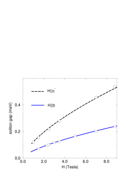
FIG. 10.: Gap of the soliton for $H\parallel c^{\prime\prime}$ and $H\parallel b$. The fits are to the simple scaling law $M\propto(H/J)^{2/3}$ as described in the text .

C Magnetic Field along $a^{\prime\prime}$ axis

For fields applied along the $a^{\prime\prime}$ axis it is impossible to obtain agreement of the MM predictions with the data. How can we understand this fact? The DM interaction is expected to lie in the $a^{\prime\prime}-c^{\prime\prime}$ plane, so that we can write

$$\vec{D}=D_{a}\vec{e}_{a^{\prime\prime}}+D_{c}\vec{e}_{c^{\prime\prime}}\ .$$ (28)

For $\vec{H}=H\vec{e}_{a^{\prime\prime}}$ the net induced staggered field is directed along the $b$ axis and is of magnitude

$$h=(0.019-2.115D_{c}/2J)H\ .$$ (29)

Clearly this would be very small if $D_{c}/J\approx 0.02$. We note that such a value of $D_{c}$ together with the gap ratio $\Delta_{{c^{\prime\prime}}}/\Delta_{b}\approx 2.2$ implies that $D_{a}/J\approx 0.12$. Note that this is consistent with the expectation that $D/J\approx.1$ and a direction of $\vec{D}$ close to the ${a^{\prime\prime}}$ axis.

In this case the coupling $\lambda(h)$ in (7) would become very small and there would be a regime in which perturbations other than the staggered field would dominate the physics. For example, if an exchange anisotropy (13) was present in Copper Benzoate, the low-energy effective theory would be given by (14) with $\mu\gg\lambda$. As a first approximation we then can ignore the $\lambda\cos\beta\Theta$ term and study the remaining (repulsive) SGM. In the framework of this scenario we obtain a rather reasonable fit to the data as is shown in Fig. 11. The expected mass gap is difficult to estimate, because as we already mentioned the coefficients in the bosonization formulas are known only in the absence of a magnectic field [16, 25, 24]. A crude estimate can be obtained by approximating the coefficents in the presence of a uniform field by the ones for $H=0$. The gaps obtained by fitting the data are found to be consistent with a rather small anisotropy $\Delta/J{<\atop\approx}0.05$ in this approximation. We note in passing that the zero-field specific heat found in [21]

$$C(T)=0.68(1)Rk_{B}T/J\ ,$$ (30)

actually corresponds to an anisotropy of the type (13) with $\Delta/J\approx 0.06$.

In order to work out a more quantitative theory for the ${a^{\prime\prime}}$-axis specific heat data the full two-frequency Sine-Gordon theory would need to be analyzed, which is possible in a perturbative framework [35]. We hope to address this point in the future. The (non) existence of the mechanism described above could in principle be checked by inelastic Neutron scattering with $\vec{H}\parallel\vec{e}_{a^{\prime\prime}}$: if the physics is indeed dominated by interactions other than the induced staggered field, the spectrum will be very different from the one oberved in [21]. In particular, if exchange anisotropy is the relevant mechanism and the effective low-energy theory is thus given by (14) with $\lambda\approx 0$, then no coherent one-particle excitations are present. The dynamical structure factor at wave number $\pi$ is then dominated by an incoherent soliton-antisoliton continuum.

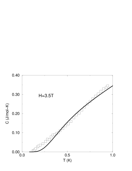
FIG. 11.: Specific heat for $H\parallel a^{\prime\prime}$. The theoretical curve is obtained by assuming an exchange anisotropy as explained in the text .

IV Conclusions

We have analyzed specific heat data for Copper Benzoate in the framework of a Sine-Gordon low-energy effective theory. For uniform magnetic fields applied along the $b$ and ${c^{\prime\prime}}$ axes we find good agreement of the theory with the specific heat data. The ${a^{\prime\prime}}$ axis data cannot be understood by the same theory that applies for the $b$ and ${c^{\prime\prime}}$ axes. We argue that the staggered field induced by the DM interaction essentially cancels the field induced by the staggered g tensor for $\vec{H}\parallel\vec{e}_{{a^{\prime\prime}}}$ so that a new mechanism is responsible for generating the gap. We propose that exchange anisotropy might be responsible.

Acknowledgements

I am very grateful to D. Reich for generously providing the experimental data and to D. Dender for many helpful explanations concerning Copper Benzoate. I also would like to thank J. Chalker and A.M. Tsvelik for important discussions and the EPSRC for support via an Advanced Fellowship.

APPENDIX A: THE HEISENBERG CHAIN IN A FIELD

We summarize some relevant results (for derivations see [15]) for the anisotropic Heisenberg model in a magnetic field

$$H_{\rm XXZ}=-4J\sum_{n}\vec{S}_{n}\cdot\vec{S}_{n+1}+(\Delta-1)S^{z}_{n}S^{z}_{n+1}-2hS^{z}\ ,$$ (31)

where $-1\leq\Delta=\cos\gamma<1$ and $J>0$. The customary form of the Hamiltonian is obtained by performing the unitary transformation

$$S_{n}^{z}\longrightarrow S_{n}^{z}\ ,\qquad S_{n}^{\pm}\longrightarrow(-1)^{n}S_{n}^{\pm}\ .$$ (32)

At low energies (31) is described by a free massless boson (1) compactified on a ring of radius $R$ i.e. $\Phi$ and $\Phi+2\pi R$ are identified. The dual field $\Theta$ fulfils $\Theta=\Theta+1/R$ (see e.g. [36]). The following bosonization rules can be derived along the lines of e.g. [37]: $\vec{S}_{n}\longrightarrow[\vec{J}(x)+\vec{n}(x)],\ x=na_{0}$, where $a_{0}$ is the lattice spacing and

$$J^{z} = \frac{a_{0}}{\beta}\partial_{x}\Phi(x)\ ,$$ (33)

$$(-1)^{n}J^{+} = i{\cal A}(\delta x)\exp\left(i\beta\Theta(x)\right)\ a_{0}\partial_{x}\Theta(x)$$ (35)

$$-\frac{{\cal B}}{2\pi}\exp\left(-i\beta\Theta(x)\right)\ \sin\left(\frac{2\pi}{\beta}\Phi(x)-2\delta x\right),$$

$$n^{x}(x) = {\Lambda_{\perp}}{}\cos(\beta\Theta(x)),\ n^{y}(x)={\Lambda_{\perp}}{}\sin(\beta\Theta(x)),$$ (36)

$$n^{z}(x) = -(-1)^{n}{\Lambda_{z}}{}\sin(\frac{2\pi}{\beta}\Phi(x)-2\delta x).$$ (37)

Here $\beta=2\pi R$ and the coefficients $\Lambda_{\perp,z}$ are known only in the absence of a magnetic field [16, 24]. The standard structure in terms of uniform and staggered magnetization operators is obtained by performing the unitary transformation (32). We note that the often neglected first term in $J^{+}$ is actually more important than the second: as a matter of fact, for $H=0$ it yields the leading contribution to transverse correlations at wave number $\pi$ of (31) [16, 38]. For $\beta=\sqrt{2\pi}$ i.e. the SU(2) invariant chain in zero field, the second term is simply the sum of left and right SU(2) currents. The first contribution to $J^{+}$ corresponds to a particle-hole excitation with spin 1 relative to the ground state (see (II.5.3) and (XVIII.1.16) of [15]) and for $H=0$ can be derived by carefully taking the continuum limit of the Jordan-Wigner lattice fermions [39, 16]. For $H\neq 0$ we expect ${\cal A}(\delta x)$ on general grounds to be of the form ${\rm const}\times\cos(2\delta x)$. Equations (37) are used to derive the continuum form of the perturbation (13) (note that both smooth and staggered components of the spin operators contribute for $\beta=\sqrt{2\pi}$).

The constant $\beta$ and spin velocity $v_{s}$ are determined by $\Delta$, $J$ and $h$ of the lattice model as follows. The dressed energy $\varepsilon$, momentum $p$ and “charge” $Z$ of an elementary spinon are given in terms of the solutions of the linear integral equations

$$\varepsilon(\lambda) - \int_{-A}^{A}\frac{d\mu}{2\pi}\ K(\lambda-\mu)\ \varepsilon(\mu)=2h-\frac{4J\sin^{2}\gamma}{\cosh 2\lambda+\cos\gamma},$$ (38)

$$p(\lambda) = 2\pi\int_{0}^{\lambda}d\mu\ \rho(\mu)\ ,$$ (39)

$$\rho(\lambda) - \int_{-A}^{A}\frac{d\mu}{2\pi}\ K(\lambda-\mu)\ \rho(\mu)=\frac{2\sin\gamma}{2\pi[\cosh 2\lambda+\cos\gamma]}\ ,$$ (40)

$$Z(\lambda) - \int_{-A}^{A}\frac{d\mu}{2\pi}\ K(\lambda-\mu)\ Z(\mu)=1\ ,$$ (41)

where $K(\lambda)=2\sin 2\gamma/(\cosh\lambda-\cos 2\gamma)$. Here $A$ is the rapidity corresponding to the Fermi momentum and is fixed by the condition

$$\varepsilon(\pm A)=0\ .$$ (42)

The spin velocity is then given by the derivative of the spinon energy with respect to the momentum at the Fermi surface

$$v_{s}=\frac{\partial\epsilon(\lambda)}{\partial p(\lambda)}\bigg{|}_{\lambda=A}=\frac{\partial\epsilon(\lambda)/\partial\lambda}{2\pi\rho(\lambda)}\bigg{|}_{\lambda=A}\ .$$ (43)

Finally, $\beta$ and $\delta$ are given by

$$\beta=\frac{\sqrt{\pi}}{Z}\ ,\ \delta=\frac{\pi}{2}-\pi\int_{-A}^{A}d\mu\ \rho(\mu)\ .$$ (44)

In order to determine $v_{s}$ and $\beta$ we solve (41) numerically, which is easily done to very high precision as the equations are linear. The results are shown in Figs 1 and 2. Finally, we note that correlation functions at small finite temperatures can be calculated like in [10] (see also [40]). We only must remember to shift the momentum by $\pm 2\delta$ away from $\pi$ for the longitudinal correlation function and use the correlation exponent as calculated above from the Bethe Ansatz. For example the transverse dynamical susceptibility at small momentum (which corresponds to momentum $\pi$ in the customary form of the Heisenberg Hamiltonian, which is related to (31) by the unitary transformation (32)) is given by

$$\chi_{\perp}(\omega,q) \propto T^{-2+\beta^{2}/2\pi}\ B(\frac{\beta^{2}}{8\pi}-i\frac{\omega-v_{s}q]}{4\pi T},1-\frac{\beta^{2}}{4\pi})$$ (46)

$$\times B(\frac{\beta^{2}}{8\pi}-i\frac{\omega+v_{s}q}{4\pi T},1-\frac{\beta^{2}}{4\pi})\ ,$$

where $B(x,y)$ is the Beta function and $q$ is close to zero. The longitudinal susceptibility is dominated by the gapless modes at $\pi\pm 2\delta$. It is the sum of two terms

$$\chi_{\parallel}(\omega,q) \propto \sum_{\sigma=\pm}T^{-2+2\pi/\beta^{2}}\ B(\frac{\pi}{2\beta^{2}}-i\frac{\omega-v_{s}Q_{\sigma}}{4\pi T},1-\frac{\pi}{\beta^{2}})$$ (48)

$$\times B(\frac{\pi}{2\beta^{2}}-i\frac{\omega+v_{s}Q_{\sigma}}{4\pi T},1-\frac{\pi}{\beta^{2}})\ ,$$

where $Q_{\sigma}=q-\pi+\sigma 2\delta$.

REFERENCES

- [1] W. Heisenberg, Z. Phys. 49, 619 (1928).
- [2] H. Bethe, Z. Phys. 71, 205 (1931).
- [3] L. Hulthén, Ark. Mat. Atron. Fys. 26A (1938).
-
[4]
C.N. Yang and C.P. Yang, Phys. Rev. 150, 321 (1966),
Phys. Rev. 150, 327 (1966), Phys. Rev. 151, 258 (1966),
S. Eggert, I. Affleck and M. Takahashi, Phys. Rev. Lett. 73 332 (1994). -
[5]
M. Takahashi, Prog. Theor. Phys. 46, 401 (1971),
J.D. Johnson and B.M. McCoy, Phys. Rev. A6, 1613 (1972),
M. Takahashi and M. Suzuki, Prog. Theor. Phys. 48, 2187 (1972),
M. Takahashi, Prog. Theor. Phys. 50, 1519 (1974). - [6] A. Klümper, preprint cond-mat/9803225.
- [7] L.D. Faddeev and L. Takhtajan, Jour. Sov. Math. 24, 241 (1984).
- [8] G. Müller, H. Thomas, H. Beck and J.C. Bonner, Phys. Rev. B24, 1429 (1981).
- [9] A. Luther and I. Peschel, Phys. Rev. B9 2911, (1974), 12 3908 (1975).
- [10] H.J. Schulz, Phys. Rev. B34, 6372 (1986).
-
[11]
A.H. Bougourzi, M. Couture and M. Kacir, Phys. Rev. B54 12669 (1996),
A. Abada, A.H. Bougourzi, B. Si-Lakhal, Nucl. Phys. B497 733 (1997). -
[12]
B.M. McCoy, J.H.H. perk and R.E. Shrock, Nucl. Phys. B220 35 (1983),
G. Müller and R.E. Shrock, Phys. Rev. Lett. 51 219 (1983), Phys. Rev. B29 288 (1984). -
[13]
M. Steiner, J. Villain and C.G. Windsor, Adv. Phys. 25 87
(1976),
S.K. Satija, J.D. Axe, G. Shirane, H. Yoshizawa and K. Hirakawa, Phys. Rev. B21 2001 (1980),
D.A. Tennant, S.E. Nagler, S. Welz, G. Shirane and K. Yamada, Phys. Rev. B52 13381 (1995),
D.A. Tennant, R. Cowley, S.E. Nagler and A.M. Tsvelik, Phys. Rev. B52 13368 (1995),
H. Yoshizawa, G. Shirane, H. Shiba, K. Hirakawa, Phys. Rev. B28 3904 (1983),
R. Coldea, D.A. Tennant, R.A. Cowley, D.F. McMorrow, B. Dorner and Z. Tylczynski, Phys. Rev. Lett. 79 151 (1997),
T. Ami, M.K. Crawford, R.L. Harlow, Z.R. Wang, D.C. Johnston, Q. Huang, R.W. Erwin, Phys. Rev. B51, 5994 (1995),
P. R. Hammar, M. B. Stone, Daniel H. Reich, C. Broholm, P. J. Gibson, M. M. Turnbull, C. P. Landee, M. Oshikawa, preprint cond-mat/9809068. -
[14]
F.D.M. Haldane, Phys. Rev. Lett. 66, 1529 (1991),
F.D.M. Haldane, Phys. Rev. Lett. 67, 937 (1991),
there is a huge literature on fractional statistics in this context, further referecens can be found in
Y.S. Wu, Phys. Rev. Lett. 73, 922 (1994),
P. Bouwknegt, A.W.W. Ludwig and K. Schoutens, Phys. Lett. B338, 448 (1994), Phys. Lett. B359, 304 (1995),
R. Kedem, T.R. Klassen, B.M. McCoy and E. Melzer, Phys. Lett. B307, 68 (1993). S. Dasmahapatra, R. Kedem, T.R. Klassen, B.M. McCoy and E. Melzer, Int. Jour. Mod. Phys. B7, 3617 (1993),
F.H.L. Eßler, Phys. Rev. B51, 13357 (1995). - [15] V. E. Korepin, A. G. Izergin, and N. M. Bogoliubov, Quantum Inverse Scattering Method, Correlation Functions and Algebraic Bethe Ansatz (Cambridge University Press, 1993).
- [16] S. Lukyanov, Nucl. Phys. B522, 533 (1998).
- [17] M. Date et.al., Suppl. Prog. Theor. Phys. 46, 194 (1970).
- [18] K. Oshima, K. Okuda and M. Date, Jour. Phys. Soc. Jpn 41, 475 (1976), Jour. Phys. Soc. Jpn 44, 757 (1978).
- [19] K. Takeda, Y. Yoshino, K. Matsumoto and T. Haseda, Jour. Phys. Soc. Jpn 49, 162 (1980).
- [20] D.C. Dender, D. Davidović, D.H. Reich, C. Broholm, K. Lefmann and G. Aeppli, Phys. Rev. B53, 2583 (1996).
- [21] D. C. Dender, P.R. Hammar, D.H. Reich, C. Broholm and G. Aeppli, Phys. Rev. Lett. 79, 1750 (1997).
- [22] M. Oshikawa and I. Affleck, Phys. Rev. Lett. 78, 1984 (1997).
- [23] The definition of the principal axes goes back to the ESR analysis of [17]. The corresponding exchange anisotropies are expected to be small (in fact too small to give rise to the gap induced by the applied field [22]), so that the isotropic Hamiltonian (2) is a natural starting point for theoretical studies of the field-induced gap.
- [24] S. Lukyanov, preprint cond-mat/9809254.
- [25] I. Affleck, Jour. Phys. A31, 4573 (1998).
-
[26]
S. Coleman, Phys. Rev. D11 2088 (1975),
S. Mandelstam, Phys. Rev. D11 3026 (1975),
R.F. Dashen, B. Hasslacher and A. Neveu, Phys. Rev. D11, 3424 (1975),
L.D. Faddeev and V.E. Korepin, Phys. Rep. 42C, 1 (1978),
V.E. Korepin, Comm. Math. Phys. 76 165 (1980),
A. G. Izergin and V. E. Korepin, Lett. Math. Phys. 5, 199 (1981),
N. M. Bogoliubov, Theor. Math. Phys. 51, 540 (1982),
V. O. Tarasov, L. A. Takhtajan, and L. D. Faddeev, Theor. Math. Phys. 57, 1059 (1984),
G.I. Japaridze, A.A. Nersesyan and P.B. Wiegmann, Nucl. Phys. B230 511 (1984),
B.M. McCoy and T.T. Wu, Phys. Lett. 87B, 50 (1979),
C. Destri and T. Segalini, Nucl. Phys. B455, 759 (1995). -
[27]
A. Luther, Phys. Rev. B14 2153 (1976),
A.B. Zamolodchikov and Al.B. Zamolodchikov, Annals of Physics 120,253 (1979),
H. Bergknoff and H. Thacker, Phys. Rev. D19 3666 (1979),
V.E. Korepin, Theor. Math. Phys. 41 169 (1979). - [28] Al.B. Zamolodchikov, Int. Jour. Mod. Phys. A10 1125 (1995).
- [29] F.H.L. Eßler and A.M. Tsvelik, Phys. Rev. B57, 10592 (1998).
-
[30]
G.I. Dzhaparidze and A.A. Nersesyan, JETP Lett. 27, 334
(1978),
V.L. Pokrovsky and A.L. Talapov, Phys. Rev. Lett. 42, 65 (1979). - [31] We set the velocity equal to one in order to simplify all equations. The velocity dependence is easily restored by dimensional analysis.
- [32] C. Destri and H.J. de Vega, Nucl. Phys. B438 413 (1995).
-
[33]
M. Suzuki, Phys. Rev. B31 2957 (1985),
T. Koma, Prog. Theor. Phys. 78, 1213 (1987),
M. Takahashi, Phys. Rev. B43, 5788 (1990),
A. Klümper, Z. Phys. 91, 507 (1993),
C. Destri and H.J. de Vega, Phys. Rev. Lett. 69 2313 (1992),
G. Jüttner, A. Klümper and J. Suzuki, Nucl. Phys. B486 650 (1997). - [34] M. Fowler and X. Zotos, Phys. Rev. B24, 2634 (1981), Phys. Rev. B25, 5806 (1982).
- [35] G. Delfino and G. Mussardo, Nucl. Phys. B516, 675 (1998).
- [36] S. Eggert and I. Affleck, Phys. Rev. B46, 10866 (1992).
- [37] A.O. Gogolin, A.A. Nersesyan and A.M. Tsvelik, Bosonization and strongly correlated systems (Cambridge University Press, 1998)
- [38] In the unitarily transformed Hamiltonian, i.e. the customary form of the XXZ Hamiltonian, this corresponds to the smooth component of transverse spin-spin correlations.
- [39] I. Affleck, Phys. Rev. Lett. 55, 1355 (1985).
- [40] R. Chitra and T. Giamarchi, Phys. Rev. B55, 5816 (1997).