Neutral evolution of model proteins: diffusion in sequence space and overdispersion.

I Introduction

A recent study on the Protein Data Bank (PDB) showed that the distribution of pairwise sequence identity between structurally homologous proteins presents a large Gaussian peak at 8.5% sequence identity, only slightly larger than what expected in the purely random case (Rost, 1998). This is an interesting result which means that the structural similarity does not imply sequence similarity.

An intensive computational study on secondary structures of RNA molecules (Schuster et al., 1994), which is a problem much simpler than protein folding, and can be studied through efficient and reliable algorithms, showed that an exponentially large number of sequences corresponds in average to a single structure, and the distribution of structures in sequence space is quite inhomogeneous (it follows a Zipf law). Sequences folding into the most common structures form connected “neutral networks” that percolate sequence space. These neutral networks directly arise from the non-uniqueness of the relation between sequence and structure.

These results are important to understand how evolution works at the molecular level. Kimura (Kimura, 1968; 1983) and Jukes and King (Jukes & King, 1969) proposed long time ago that most of the evolutionary events at the molecular level are non Darwinian. They consist in the substitution of one allele with another one selectively equivalent (neutral evolution). The keystone of neutral evolution is the existence of a “phenotypic threshold”. The phenotypic threshold is defined in terms of similarity between structures. Below a critical value of structural similarity, natural selection cannot avoid the spreading of variants of the protein in a population through “diffusion”, called by genetists “genetic drift” (such threshold may depend on the size of the population and on the mutation rate). Neutral evolution in sequence space conserves the structure of the protein (thus taking place below the phenotypic threshold) but can drive to sequence similarities expected for randomly chosen sequences.

The purpose of this paper is to investigate these questions in a simplified model of protein folding. Our aim is to show that, as in the case of RNA sequences, protein sequence space is traversed by vast neutral networks.

The attempt to study this problem requires some methodological choices. The first and most severe condition is that, given a sequence of amino acids, we should be able to identify its native conformation. This is tantamount of solving the protein folding problem. We decided to adopt a lattice model of proteins, since, to date, this is the only case in which protein folding is routinely solvable. This choice restricts drastically the possibility to represent active sites and structural motifs, which might play an important role in constraining neutral evolution.

The second choice is how to represent mutations. We mutate amino acids and not nucleotides. In nature mutations affect DNA, so that mutations happen with larger frequency between amino acids whose codes differ by just one nucleotide. We do not take this fact into account and consider an uniform probability of mutation for any nucleotide. This does not change the characteristics of the “neutral networks”, and it should not change the relevant features of diffusion in sequence space. Moreover, we work with sequences of fixed length (number of amino acids) $N=36$, considering only point mutations, without insertions and deletions.

The third choice is how to represent the phenotypic threshold. We introduce a stochastic algorithm which at each time step attempts to change one amino acid. The mutation is accepted if three conditions are met: the ground state should be conserved, thermodynamically stable and easily accessible.

Since we are limited by computational resources, we decided to study one particular neutral network. Namely we followed the evolution from one single common ancestor. The extent to which this network can be considered paradigmatic will be commented.

We believe that the features of neutral evolution which are found in real proteins are universal enough to be captured by the present simplified model. Support to this view comes from a recent study by Babajide and coworkers (Babajide et al., 1997). They also found evidence for the presence of neutral networks in sequence space. Their work is similar in spirit to the present one, but significantly different methodologically. They used a description of the protein structure based on the $C_{\alpha}$ and $C_{\beta}$ coordinates as taken from the PDB, and an approximate criterion of fold recognition based on the Z score (Bowie et al., 1991; Casari & Sippl, 1992).

The paper is organized as follows: in Sec. II, we present an outline of the theory of neutral evolution. In Sec. III, we describe our model protein and our protocol to simulate neutral evolution. In Sec. IV we illustrate our results concerning the genetic drift. In Sec. V we deal with population genetic considerations and study the dispersion index of the process of substitutions. Sec. VI presents an overall discussion, where we discuss the applicability of our results to the interpretation of existing biological data.

II The neutral theory of evolution

The theory of evolution explains how different living species evolve adapting to an ever changing environment. The key ingredients of the explanation are reproduction, mutation and natural selection, and the complex ecological interactions that modify the environment. The pattern of change in time at the phenotypic level is quite irregular: long periods of stasis are followed by abrupt bursts of activity, species suddenly appear and disappear and very large extinction events happen, showing complex features (Gould & Eldredge, 1977; Solé et al., 1997). In contrast to this, evolution at the molecular level seems to be much more regular. The first studies on this subject showed that the rate of change in time of the amino acid sequence of a given protein, which can be estimated from the difference of homologous sequences of different species, in most cases does not vary much from one species to another in the same class, even if the species compared have rather different population size and environmental conditions (Zuckerland & Pauling, 1962) (on the other hand, the evolution rate changes drastically from one protein to another). This property makes each protein a sort of “molecular clock” (Zuckerland & Pauling, 1962; Kimura, 1983; Gillespie, 1991; Ratner et al., 1996), with its own measure of time, and allows to transform a distance in sequence into a distance in time and to reconstruct phylogenetic trees from molecular data.

In order to explain this and other features of molecular evolution, as for example the presence of many polymorphic loci in the genome, thirty years ago Kimura (Kimura, 1968) and Jukes and King (Jukes & King, 1969) proposed a new and at that time “revolutionary” interpretation of molecular evolution, that was named the neutral theory of molecular evolution, reviewed in (Kimura, 1983). According to this theory, most of the changes in protein sequences happen not because better variants of the protein are found and spread in the population by natural selection, but because many mutations do not modify significantly the efficiency of the protein, so that natural selection cannot avoid their spreading through the population by random genetic “drift” (“diffusion” in physical language).

One decade later, the theory of the molecular quasi-species (Eigen et al., 1989) showed the possible existence of an evolutionary phase, at high mutation rate and low selective pressure, with the diffusive features of neutral evolution: thus this mode of evolution is expected not only for strictly neutral mutations, but whenever the damage brought by frequently occurring mutations is smaller than a threshold depending on the mutation rate. With regard to proteins, in the framework of their random heteropolymer model, Shakhnovich and Gutin estimated the probability of a mutation which does not change the ground state (Shakhnovich & Gutin, 1991). Their conclusion is that this probability has a finite limit for increasing system size.

There have been however more recent and accurate studies which question the very existence of molecular clocks, noting that most of the clocks underwent in some instances (i.e. in some periods of the evolution of some lineages) drastic accelerations or decelerations (Ayala, 1997) so that the usefulness of the clock hypothesis to reconstruct evolution is very reduced. In some cases, the adaptive nature of the acceleration of the substitution rate was clearly demonstrated, like in the case of the changes that hemoglobin underwent in the time when vertebrates colonized the earth (Ratner et al., 1996). According to the selectionist interpretation, these discrepancies of the clocks are such that the neutral hypothesis should be completely rejected. This dispute produced a vast literature (see the book by Gillespie (Gillespie, 1991) for a nice and richly detailed discussion of the selectionist point of view).

In this work we take a different point of view, and investigate with a minimal model the possibility of neutral evolution of proteins. We find that the model supports this possibility. Interestingly, we find also that the rate $R$ between the variance of the number of substitutions and its average value is larger than 1. Originally, Kimura proposed that the substitution of amino acids in proteins follows a Poissonian stochastic process, which implies $R=1$. For most proteins however real data give $R$ significantly larger than 1, till values between 30 and 50 (Gillespie, 1991) (this problem is produced by the drastic accelerations of the substitution process mentioned above). This was considered as a severe evidence against the neutral theory. Thus it is remarkable that a “microscopic” model which considers only the possibility of neutral evolution leads to results that reconcile the neutral theory with at least part of the data.

Finally, a remark about terminology: by “mutation” we mean the modification of a triplet of the genetic code in one individual lineage (by means of environmental damages, errors in the replication process or other causes). By “substitution” we mean the much more complex process in which an allele dominant in a biological population is replaced by a new one arising from mutation. We consider here only individual lineages. Passing from the level of individual lineages (mutation and reproduction) to the level of a population (substitution) requires the tools of population genetics. However, Kimura (Kimura, 1968; Kimura, 1983) showed that the passage is very simple in the case in which the only mutations occurring are either lethal or completely neutral for natural selection. In this case, the substitution rate in the population is

$$\mu_{subs}=\mu x,$$ (1)

where $\mu$ is the “microscopic” mutation rate (at the level of the single lineage) and $x$ is the fraction of mutations which are selectively neutral (see also (Bastolla & Peliti, 1991)). Note that the rate of evolution does not depend on the size of the population, whereas it does if positive natural selection plays a role.

Under these assumptions, the model of neutral evolution of single lineages that we present here is equivalent to a model of evolution at the level of a population, and thus it can be in principle compared to biological data.

III Model of neutral evolution in proteins

In this section we give a detailed description of the lattice model we used to represent proteins and of the algorithm we introduced to study evolution in sequence space.

A Definition of the model proteins

In our model, a protein configuration is represented by a self avoiding walk on the simple cubic lattice. Each of the $N$ occupied sites represents an amino acid, chosen among the 20 possible ones. We represent a configuration of the protein by its contact map ${\bf C}$. This is a $N\times N$ matrix whose element $C_{ij}$ is 1 if residues $i$ and $j$ are nearest neighbors on the lattice (but not along the chain) and 0 otherwise. Note that the correspondence between contact maps and configurations is not unique, and the smaller is the “density of contacts” $N_{c}/N$ of a contact map, where $N_{c}=\sum_{i<j}C_{ij}$ is the number of contacts, the larger is the number of configurations to which it corresponds (Vendruscolo et al., 1998).

We denote a sequence of length $N$ by ${\bf S}=\{s_{1},\ldots,s_{N}\}$. An energy $E({\bf S},{\bf C})$ is assigned to sequence ${\bf S}$ on a configuration whose contact map is ${\bf C}$

$$E({\bf S},{\bf C})=\sum_{i<j}^{1,N}C_{ij}U(s_{i},s_{j})\,.$$ (2)

where $U(a,b)$ is a $20\times 20$ symmetric interaction matrix, which gives the energy gain obtained when amino acids of species $a$ and $b$ are brought into contact. We use a matrix $U(a,b)$ derived from the Miyazawa-Jernigan interaction matrix (Miyazawa & Jernigan, 1985). In our model, we identify the ground state structure as the native structure.

We now define two measures of similarity respectively in sequence space and in structure space. The standard measure of similarity between two sequences ${\bf S}$ and ${\bf S}^{\prime}$ of the same length $N$ is the Hamming distance, which counts the number of amino acids which are different:

$$D({\bf S},{\bf S}^{\prime})=\sum_{i=1}^{N}\left[1-\delta(s_{i},s^{\prime}_{i})\right]\;,$$ (3)

where $\delta$ is the Kronecker symbol and $s_{i}$ takes 20 different values. We also consider the overlap $Q({\bf S},{\bf S}^{\prime})$,

$$Q({\bf S},{\bf S}^{\prime})={1\over N}\sum_{i=1}^{N}\delta(s_{i},s^{\prime}_{i})\;,$$ (4)

which is equal to 1 minus the normalized Hamming distance $D/N$.

In sequence space, we introduce also two alternative measures of similarity, $D_{HP}({\bf S},{\bf S}^{\prime})$ to measure differences in hydrophobicity. and $D_{U}({\bf S},{\bf S}^{\prime})$ to measure the difference in the native interactions. To define $D_{HP}({\bf S},{\bf S}^{\prime})$ we transform every sequence into a sequence of binary symbols, either H or P, according to the hydrophobicity of the residue. We consider 8 hydrophobic amino-acids and 12 polar ones. The definitions of $D_{HP}({\bf S},{\bf S}^{\prime})$ and of the related overlap $Q_{HP}({\bf S},{\bf S}^{\prime})$ are analogous to those of $D$ and $Q$, where now $s_{i}$ can take only two values. The distance $D_{U}({\bf S},{\bf S}^{\prime})$ is given by the quadratic difference of the native interactions in two different sequences:

$$D_{U}({\bf S},{\bf S}^{\prime})=\sum_{i<j}{\bf C}^{*}_{ij}\left[U(S_{i},S_{j})-U(S^{\prime}_{i},S^{\prime}_{j})\right]^{2}\;,$$ (5)

where ${\bf C}^{*}$ is the native contact map.

We measure similarity in configuration space by the overlap $q({\bf C},{\bf C}^{\prime})$ between contact maps ${\bf C}$ and ${\bf C}^{\prime}$

$$q({\bf C},{\bf C}^{\prime})={1\over N_{c}^{*}}\sum_{i<j}C_{ij}C^{\prime}_{ij}\;,$$ (6)

where $N_{c}^{*}$ is the maximal between $N_{c}$ and $N_{c}^{\prime}$, the number of contacts respectively of two contact maps ${\bf C}$ and ${\bf C}^{\prime}$. Two maps are identical if and only if $q=1$.

We consider a sequence with $N=36$ and a contact map ${\bf C}^{*}$ which has the highest possible number of contacts for this chain length, $N_{c}=40$. (See Fig. 1). In this case the contact map defines uniquely the configuration of the system (apart from trivial symmetries).

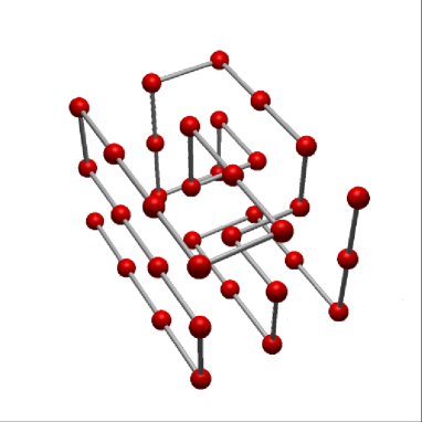
FIG. 1.: The “native state” of our model protein

The contact map $C^{*}$ was studied by Shakhnovich and coworkers in a computer experiment of inverse folding (Abkevich et al., 1994). They designed a sequence ${\bf S}^{*}$ with ground state on ${\bf C}^{*}$ using the procedure of (Shakhnovich & Gutin, 1993), showing that ${\bf S}^{*}$ has good properties of kinetic foldability and thermodynamic stability at the temperature where the folding is fastest. The lower part of the energy landscape of this sequence is remarkably smooth: all the structures with low energy have a high overlap $q_{0}$ with the ground state. The lowest energy of configurations with a fixed value of $q_{0}$ decreases regularly as $q_{0}$ approaches one. This correlated energy landscape, reminiscent of the “funnel” paradigm (Bringelson & Wolynes, 1987), is the reason of the good folding properties of the sequence, which is very different from a random one. In (Tiana et al., 1998) it was shown that the same sequence is also very stable against mutations. It was estimated that about 70% of the point mutations performed on ${\bf S}^{*}$ result in a new sequences with exactly the same ground state and good folding properties. Thus energy minimization makes ${\bf C}^{*}$ stable not only in structure space, but also in sequence space.

We note that ${\bf C}^{*}$ is a rather atypical structure for the interaction parameters that we choose: since $U(a,b)$ has average value zero and variance $0.3$, we would expect open structures to be energetically favored. Indeed, typical random sequences with $N=36$ and contact interactions whose average vanishes have a ground state with approximately 30-32 contacts (Bastolla, unpublished result), being thus less than maximally compact.

B Definition of the model of evolution

We consider a reference contact map ${\bf C}^{*}$ as the biologically active native structure, and we set as starting point of neutral evolution a sequence ${\bf S}^{*}$ which folds onto ${\bf C}^{*}$.

The simulated molecular evolution is realized by the following iterative procedure

1. At $t=0$ we start from ${\bf S}(0)={\bf S}^{*}$.

2. At time step $t$ we mutate at random one amino acid of ${\bf S}(t-1)$, producing a new sequence ${\bf S}^{\prime}(t)$.

3. We submit the new sequence to selection according to the criteria specified below. If the sequence survives then ${\bf S}(t)={\bf S}^{\prime}(t)$, otherwise we restore ${\bf S}(t)={\bf S}(t-1)$.

The selection of sequences is governed by the following conditions:

  

Conservation of the phenotype.

The ground state ${\bf C}$ of ${\bf S}^{\prime}(t)$ must have an overlap with ${\bf C}^{*}$ not smaller than a given “phenotypic threshold” $q_{\rm thr}$.

$$q({\bf C}^{*},{\bf C})\geq q_{\rm thr}\;,$$ (7)

In our calculations we imposed strict conservation of the phenotype by setting $q_{\rm thr}=1$.

  

Thermodynamic stability.

We define thermodynamic stability through the condition

$$\left\langle q({\bf C}^{*},{\bf C})\right\rangle\geq\langle q\rangle_{\rm thr}\;,$$ (8)

where $\langle\cdot\rangle$ represent a Boltzmann average at the temperature $T$ of the simulation and $\langle q\rangle_{\rm thr}$ is a fixed parameter. This condition implies that all the thermodynamically relevant states have an overlap greater than $\langle q\rangle_{\rm thr}$ with the target state.

  

Kinetic accessibility.

We use the PERM method (Grassberger, 1997; Fraeunkron et al., 1998; Bastolla et al., 1998), a new Monte Carlo algorithm which is particularly successful in finding the ground state of lattice polymers. For every sequence ${\bf S}$ to be tested, we run $\tau$ iterations of the algorithm. If the lowest energy structure found at this point does not coincide with ${\bf C}^{*}$, we discard the sequence because the kinetic accessibility condition is violated. Otherwise, we continue to run the algorithm for a time $\tau$ to check that no lower energy structure is found. If this condition is met, we start again the algorithm and run it for a time $2\tau$. Only if ${\bf C}^{*}$ is once again found as the lowest energy structure we conclude that the ground state of ${\bf S}$ really coincides with ${\bf C}^{*}$. Note that there is no bias towards ${\bf C}^{*}$ in our Monte Carlo algorithm.

We never found in the second independent run of the MC algorithm a structure with lower energy than the putative ground-state ${\bf C}^{*}$. This fact encourages us in believing that the algorithm was really effective in finding the ground state. Another support to this conclusion comes from the fact that all of the selected sequences had a remarkably correlated energy landscape, which makes the search for the ground state easier. On the other hand, whenever a sequence was rejected, we are not sure whether we were able to determine its ground state. The difference is due to two reasons: first, we run rejected sequences for a shorter time ($\tau$ instead of $2\tau$ is the rejection is made at the first decision stage, 1 run instead of 2 independent ones if it is made at the second stage). Second, rejected sequences have typically a much less correlated energy landscape, so that it is expected that the determination of the ground state is more difficult. Nevertheless, we shall discuss at the end also data about rejected sequences, since they are interesting and refer to a very large number of sequences, even if they are individually not completely reliable.

The 3 conditions for the acceptance of a mutation enforce the conservation of biological activity of the new sequence. We have to stress that conservation of the fold is not a necessary condition for selective neutrality in the real world, and it is not even sufficient, since the active site has also to be conserved and the environment has to remain reasonably stable. Thus with our model we can represent just the neutral evolution of the part of the chain not involved in chemical activity, in a stable chemical environment. Nevertheless, we think that these limitations do not prevent from the applicability of the model to real molecular evolution.

C Genetic drift

For a given sequence ${\bf S}$ of $N$ amino acids, we define the rate of neutral mutation $x$ as the fraction of acceptable non-synonymous mutations

$$x({\bf S})=\frac{1}{20N}\sum_{i=1}^{N}\sum_{\alpha\neq s_{i}}^{1,20}\chi_{i}^{\alpha}\;,$$ (9)

where $\chi_{i}^{\alpha}=1$ if assigning the amino acid of species $\alpha$ at position $i$ on the sequence does not change the native state and 0 otherwise. In Kimura’s ordinary neutral theory (Kimura, 1983) it is assumed that $x({\bf S})=x$ is indeed independent of the sequence. With this hypothesis, the evolution of the overlap from the starting sequence $\overline{Q(t)}=\overline{Q({\bf S}(0),{\bf S}(t))}$ (the overbar denotes an average with respect to the mutation process) is given by

$$\overline{Q(t)}\approx{1\over 20}+\left(1-{1\over 20}\right){\rm e}^{-xt/N}\;.$$ (10)

Since every mutation is either neutral or lethal, the evolution of the wild-type genome of the population coincides with that of a single reproductive line (Kimura, 1983), and we may interpret different realizations of our evolutionary process as different ‘species’ originating from a common ancestor. Thus $\mu_{subs}=x/N$ is the substitution rate both of a single lineage and of the population, and the time $t$ represents in our model the number of mutational events. As we shall see, however, the hypothesis of constance of $x({\bf S})$ is not in agreement with the results of the simulations.

D Neutral set

We define the neutral network $\omega({\bf C}^{*},{\bf S}^{*})$ as follows:

$\omega({\bf C}^{*},{\bf S}^{*})$ is formed by all the sequences ${\bf S}$ that have ${\bf C}^{*}$ as their ground state and are connected to ${\bf S}^{*}$ through a neutral path (a path in sequence space which satisfies the three selection criteria given above).

We then define the neutral set $\Omega({\bf C}^{*})$ as

$$\Omega({\bf C}^{*})=\cup_{\mu}\omega({\bf C}^{*},{\bf S}_{\mu}^{*})$$ (11)

with $\mu$ running over different sequences ${\bf S}_{\mu}^{*}$ with ground state on ${\bf C}^{*}$ but not connected by neutral paths. It is possible that this set is larger than the neutral network of a single sequence, $\omega({\bf C}^{*},{\bf S}^{*})$. In this case it would be possible in principle to distinguish between convergent (different ancestors, same final structure) and divergent (same ancestor) evolution: if the evolution of two homologous proteins takes place in two disjoint neutral networks, it must be convergent.

We studied only one starting sequence ${\bf S}^{*}$, thus this work is concerned only with divergent evolution. However, since the neutral networks that we studied is so spread that typical pairs of sequences have a Hamming distance comparable with that of random sequences, it turns out that it is not possible to distinguish between divergent and convergent evolution on the basis of the sequence homology alone. Under this respect, our results are equivalent to those of Rost (Rost, 1997).

IV Results

A Evolutionary drift

We generated 8 trajectories with the following values of the selection parameters: $q_{\rm thr}=1$, $\langle q\rangle_{\rm thr}=0.9$, $T=0.16$, $\tau=1.6\cdot 10^{5}$. In each trajectory, a number of sequences ranging from 875 to 2709 were tested. The CPU time needed for a single trajectory was about 4 to 5 weeks on Sun Ultra stations.

Different realizations differentiated greatly from the “common ancestor” ${\bf S}(0)$ and from each other. We give three measures of such differentiation. 1) The average Hamming distance between the final points of the 8 evolutionary trajectories is $D_{H}=30.2$, which is only 12% smaller than the random value $D_{H}^{ran}=34.2$. 2) The maximum distances from the starting point in the 8 trajectories are respectively 26, 28, 27, 27, 17, 33, 25, and 23. 3) The maximum distance between sequences in different trajectories ranges from 27 to 35. We note that these values were still increasing as a function of the length of the simulations when we had to stop them, so that it is possible that their asymptotic values for very long trajectories are compatible with those of random samples of sequences. Moreover, the trajectories were run for different mutational times.

Fig. 2a shows the distribution of the distance among the end points of independent trajectories, both with the full 20 letters alphabet (white bars) and with the coarse-grained hydrophobic representation (black bars). In the latter, the average value is $D_{HP}=16.3$, not far from the random value $D_{HP}^{ran}=17.3$, and the variance is $V_{HP}=6.0$, compatible with $V_{HP}=D_{HP}(1-D_{HP})/N$. In both cases, the typical values for random sequences are larger than the typical values we found, but this could be due to the fact that our simulations did not last a time long enough to equilibrate. It is surprising that also the hydrophobic distance is close to that expected for random sequences. This is probably an effect of the short length of our sequences whose ground states have at most 2 residues in the core, while all other ones are at the surface. The two residues at the core are the most conserved during the evolution (see next subsection). However, we observe that even one of these residues could be replaced in some instances with hydrophilic residues.

In Fig. 2b we show the relaxation of the overlap $Q({\bf S}(0),{\bf S}(t))$ for three trajectories. The differences from one realization to another are quite large, but at large times the trajectories show the tendency to converge together.

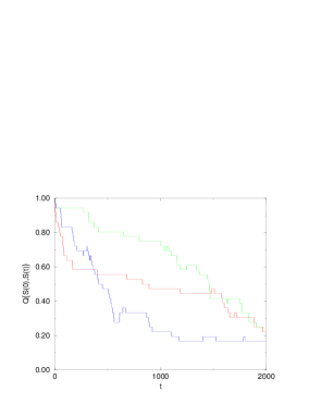
FIG. 2.: (a): Histograms of the Hamming distances between the end points of independent trajectories with the full 20 amino-acid alphabet (white) and with a reduced 2 amino-acid alphabet (black). The dashed lines indicate the most probable values of the distance for random pairs (b): Decay of the overlap with the starting sequence for 3 independent trajectories.

In Fig. 3a we show the Hamming distance $D({\bf S}(0),{\bf S}(t))/N$ averaged over 8 trajectories and we compare it with the interaction distance $D_{U}/6$ (Eq. 5). The temporal behavior is very similar in the two cases, although the maximum value reached in the case of $D_{U}$ is 5.6, roughly half of the naive expectation for random sequences given by the number of native contacts (40) multiplied by the variance of the interaction matrix (0.3). In Fig. 3b we show $D(t_{0},t)/N=1-Q({\bf S}(t_{0}),{\bf S}(t_{0}+t))$, averaged over all the trajectories generated. There is a systematic dependence on $t_{0}$ at small $t$: the larger is $t_{0}$, the slower is the initial relaxation. We believe that this result is due to the fact that ${\bf S}(0)$ is quite a peculiar starting point, much more stable with respect to point mutations than other sequences in $\omega({\bf C},{\bf S}(0))$. Thus, as the trajectories go further away from ${\bf S}(0)$, the rate of accepted mutations decreases. On the other hand, the different curves meet again at large $t$. This could be due to the fact that at large $t$ a large portion of sequence space has been explored, and the rate of accepted mutations has been averaged over this large region.

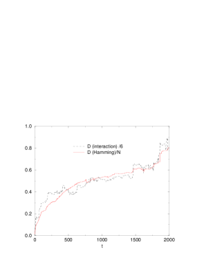
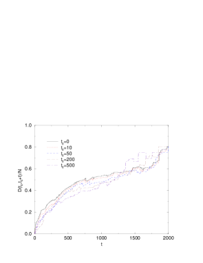
FIG. 3.: (a): Interaction distance (quadratic difference of the native interactions) from ${\bf S}(0)$ compared with the Hamming distance. (b) Distance averaged over different trajectories from different sequences ${\bf S}(t_{0})$.

The relaxation in Fig. 3a is not exponential, as it would be if the probability $x$ of a neutral mutation were almost constant for all sequences. In fact, as we shall see, the quantity $x$ defined in Eq. 9 has a very broad distribution in sequence space, and the simple expectation (Eq. 10) does not hold.

B Rigidity

We define the rigidity $R_{i}$ as a measure of the degree of conservation of residue $i$:

$$R_{i}=\sum_{a}P_{i}^{2}(a)\;,$$ (12)

where $P_{i}(a)$ is the probability to find the amino-acid $a$ at position $i$. $P_{i}(a)$ is estimated from the end points of the 8 neutral paths we generated. $R_{i}=1$ if the amino-acid at position $i$ is never changed, while $R_{i}=1/20$ if it is completely random. We show in Fig. 4 that all the amino acids could be changed at least once, even if the value of $R$ is typically 3 to 5 times larger than for a random distribution, and some sites are very stable. Not surprisingly, the two most stable sites are in the ‘core’ of the protein. One of them has already been found to be particularly sensitive to mutations concerning ${\bf S}(0)$ (a red site, in the terminology of Tiana et al.). It is remarkable that, even if the second core site was not very sensitive to mutations in ${\bf S}(0)$ (it was classified as a yellow site), we find that it is strongly conserved in the overall evolution. Fig. 4a shows the rigidity for the 20 letter alphabet.

In Fig. 4b we show the rigidity for the coarse-grained HP alphabet. This is of course larger than in the case of 20 letters. Many residues have a rigidity compatible with the random value $R_{HP}=0.52$, and the hydrophobicity of every residue was changed at least once in the course of evolution (even if amino acid 32 is always polar in all of the 8 final sequences). At first glance these results seem surprising, since one would expect that the hydrophobic pattern should be more conserved during evolution than we actually found. However, our model protein is quite small, and its hydrophobic core is constituted by only 2 sites, whose rigidity is much larger than random, and it is not strange that the hydrophobic pattern of most of the other residues is close to a random one.

FIG. 4.: Rigidity at different positions (see text) for (a) the full 20 amino-acids alphabet and (b) a reduced HP alphabet. The peaks in (a) correspond to the two core positions.

C Neutral Mutation Rate

The simplest measure of the neutral mutation rate $x$ (Eq. 9) is obtained by computing the frequency of neutral mutations over all the non-synonymous mutations proposed. In this way we found $\overline{x}\approx 0.06$ (the overline represents an average over the mutational process). However, this quantity alone is not enough to characterize $x$, which fluctuates strongly in sequence space. For instance, it was estimated by one of us and coworkers (Tiana et al., 1998) that $x({\bf S}^{*})\approx 0.7$, where ${\bf S}^{*}$ is the starting point of all our evolutionary trajectories.

In order to see whether $x({\bf S})$ has some structure in sequence space, we divided the sequences ${\bf S}\in\omega({\bf C}^{*},{\bf S}(0))$ in every trajectory in groups of 100 sequences, as long as they are generated, and we stored the average fraction of successful mutations in each group, $x(r)$ (where $r$ labels the sequences in the order in which they are generated). It appears that the first groups of sequences have a rather high value of $x$, but this value quickly decreases, and then $x(r)$ seems to fluctuate more or less randomly.

FIG. 5.: Variation of $x(S)$ in sequence space.

We also measured indirectly the distribution of $x({\bf S})$ in sequence space from the distribution of the “trapping” time $\tau_{j}({\bf S})$ that a trajectory spends on sequence ${\bf S}$. The average value of the trapping time is inversely proportional to the neutral mutation rate (we neglect in this argument the randomness given by the error in evaluating whether a sequence belongs to the neutral set: in particular, the conditions of fast folding and of thermodynamic stability are subject to considerable evaluation errors):

$$\overline{\tau_{j}({\bf S})}=\frac{1}{x({\bf S})}\;,$$ (13)

where the bar denotes average over different attempts to mutate sequence ${\bf S}$. These attempts are unsuccessful with probability $1-x({\bf S})$, so that the probability that the first successful mutation is met at trial number $\tau$ is given by the geometric distribution,

$$P_{x}(\tau)=x(1-x)^{\tau-1}\>.$$ (14)

Averaging in sequence space, we get

$$\left[P(\tau)\right]=\int_{0}^{1}dx~{}p(x)\left(x\over 1-x\right)(1-x)^{\tau}\;,$$ (15)

where $\left[\cdot\right]$ denotes an average over sequences belonging to the neutral network $\omega({\bf C}^{*},{\bf S}(0))$. We found that the distribution of $\tau_{j}$ is very broad. It seems to be broader than an exponential (see Fig. 6), thus, even if we cannot invert Eq. 15, we expect that the distribution of the neutral mutation rate $x$ is also broader than exponential.

FIG. 6.: Distribution of the trapping time $\tau_{j}$.

We measured also the correlations of $\tau_{j}$ in sequence space,

$$C_{\tau}(l)={\overline{\tau_{j}(r)\tau_{j}(r+1)}\over\overline{\tau_{j}(r)}^{2}}-1\;.$$ (16)

There is a positive correlation after one step in sequence space, $C_{\tau}(1)\approx 0.98$, but after few steps the correlation vanishes (data not shown).

D Rejected sequences

As the last point, we want to report briefly results regarding the sequences that were rejected by our selection algorithm. More details about this point and about properties of selected sequences will be given in a forecoming publication. As we said, results concerning rejected sequences are not completely reliable, since in this case the identification of the ground state is only tentative. However, they represent about $94\%$ of the $12,000$ sequences that we generated, and the statistical properties of this large set are interesting and qualitatively clear. The most interesting observation concerns the overlap $q_{0}=q({\bf C}^{*},{\bf C}_{0})$ measuring the similarity between the ground states ${\bf C}_{0}$ of our sequences and the target structure ${\bf C}^{*}$. This has a bimodal distribution, with a high peak at $q_{0}=1$ (more than 16% of the rejected sequences), corresponding to sequences that have ground state on ${\bf C}^{*}$ but do not fulfill either the condition of thermodynamical stability or that of fast folding. This peak has a sudden drop and then it decreases slowly at decreasing $q_{0}$. At $q_{0}=0.32$ a new peak is present, related to ground states which have less contacts than ${\bf C}^{*}$ (the typical value is 34 instead of 40), but more than it is expected in the ground state of random sequences. These structures are more similar to typical low energy structures than to the target state. Thus, even if a large fraction of mutations conserves the ground state, the majority of them produces very large structural changes.

The energy of the ground state is strongly correlated both to the similarity $q_{0}$ to the target and to the number of contacts $N_{c}^{0}$ (in fact, the latter two quantities are strictly related). Only in few cases we found sequences with very low ground states that are unrelated to the target: for instance, in two cases we found energies lower than -17 with $q_{0}$ as low as $.5$ and $.35$ respectively. From this observation we speculate that it is unlikely (although not excluded) that two neutral sets of stable and unrelated structures can be close to each other. In this sense, our result is related to those of (Li et al., 1998).

V Overdispersion and population genetics considerations

In the previous sections, we described the evolution of a single lineage of a protein, subject only to lethal and neutral mutations. As we mentioned in Sec. II, under these hypothesis the evolution at the level of the population happens with the same rate as the evolution of a single lineage. Thus we can interpret our 8 evolutionary trajectories as 8 species differentiating from a common ancestor (star phylogeny), and compare our data to real evolutionary rates.

In order to do this comparison, we have to further elaborate on the model for mutations. Time in the model is measured as the number of mutation events, and we have to relate this number to real time. The simplest possibility is to assume that the number of mutations in the geological time $T$ is a Poissonian variable with average value $\mu T$. This assumption is similar to Kimura’s one, but in his model the fraction of neutral mutations $x$ is considered constant throughout the evolution, while our results show that this quantity is strongly fluctuating.

Thus we simulate the evolution of a star phylogeny by extracting 8 Poissonian variables with average value $\mu T$, $t_{1}\cdots t_{8}$. The number $S_{i}(t_{i})$ of substitutions fixed after $t_{i}$ mutational events in the $i-$th trajectory is then interpreted as the number of substitutions in the species $i$.

We measure as a function of $T$ the ratio $R(T)$ between the variance and the mean value of $S$

$$R(T)=\overline{\left\langle S^{2}\right\rangle-\left\langle S\right\rangle^{2}\over\left\langle S\right\rangle}\;,$$ (17)

where the angular brackets denote the average respect to the 8 species in our population and the overline denotes an average respect to 1000 extractions of the Poissonian variables. The resulting curve is shown in Fig. 7.

FIG. 7.: Dispersion index $R(T)$ as a function of geological time $T$, as defined in Eq. 17.

If we assume that the mutations are mainly due to errors in the replication accuracy, we should consider that $\mu=\mu_{i}$ depends on the duration of a generation for species $i$ (in particular, it should be inversely proportional). This is the generation time effect, that has been shown to be present in real evolutionary data (Otha, 1993) and to be stronger for synonymous mutations (for which $x=1$) than for non-synonymous mutations, which are the subject of our study. We do not consider here this effect, essentially for two reasons:

1. The mutation rate should also increase with the number of mitosis preceding reproduction, and this number is larger the larger the generation time. Thus the generation time effect is reduced in many cases.

2. It was shown that the dispersion index $R(T)$ is significantly larger than unity even when the generation time effect and other lineage-depending effects are taken into account (Gillespie, 1991). Gillespie named “residual dispersion index” the quantity $R(T)$ computed removing all lineages effects. Considering the same rate of mutation for all “species”, we aim to study residual effects, which are most critical with respect to the neutral theory.

A last point remains to be made. Since $x$ has strong fluctuations, it follows that the sequences in the neutral sets are not equivalent: sequences with a large value of $x({\bf S})$ should be advantageous because their offsprings suffer a smaller fraction of genetic deaths. Thus it could be thought that the population localizes in a region of sequence space where $x({\bf S})$ is large, so that the evolution is not anymore neutral at the level of population genetics. However, we think that such phenomenon cannot take place. In fact, the selective advantage of sequences with large $x({\bf S})$ is proportional to the mutation rate $\mu$. But it is known, for instance from the theory of the error threshold (Eigen et al., 1989), that there is a minimum selective advantage $u(\mu)$, increasing with the mutation rate, below which natural selection is not able to fix advantageous genotypes. We expect that the selective advantage implied by a larger $x({\bf S})$ is always below the error threshold. Moreover, since $x({\bf S})$ is a rather correlated quantity in sequence space, and since the alleles present in a finite population should be related through few mutations, the effective selective advantage, related to the difference between the $x({\bf S})$ of the alleles in the population, should be very small.

This effect however could act as a kind of negative feedback, reducing the effect of the variations of $x$ on the variation of the substitution rate. Another small reduction, present even when $x$ is constant in the population, is due to a small correction to Kimura’s formula (Eq. 1). It was shown in (Bastolla & Peliti, 1991) that the substitution rate of a protein in a large population of asexually reproducing individuals, evolving in a sequence landscape with sharply distributed $x({\bf S})$, is given by

$$\mu_{subs}=\mu x/(1-\delta)\;,$$ (18)

where $\delta\approx\mu N(1-x)$ is the fraction of the population eliminated by lethal mutations. The factor $1/(1-\delta)$ is due to a normalization condition: the larger is $\delta$, the easier is for the individuals who suffered a neutral mutation to spread their genome in the population. Thus the effect of a variation in $x$ on the mutation rate is, in the case of a population, smaller than in the case of a single reproductive lineage, where $\mu_{subs}=\mu x$, and the dispersion index should be consequently slightly smaller.

Despite of these caveats, we think that our results are applicable also at the level of population genetics.

VI Discussion

We studied neutral evolution in sequence space. The theory of neutral evolution states that the mutations that do not affect the biological activity of the protein are much more frequent than advantageous mutations. In our model the latter are not represented: all mutations that are not neutral are assumed to be lethal. Neutrality is tested imposing the conservation of the tridimensional structure, of its thermodynamic stability and its kinetic accessibility. Two main messages emerge.

The first one is that large differences in the genotype (viz the sequence) are compatible with conservation of the phenotype (viz the native structure). The set of sequences which fold onto the same structure and are connected through point mutations is extended to form a vast network in sequence space. Two typical sequences belonging to this set, even if they are evolutionarily related, may have a degree of homology as low as that of random sequences. Thus sequence similarity is not a necessary condition for two proteins being evolutionarily related.

The second message is that neutral evolution can be very irregular. We have shown that the fraction of neutral mutations is a strongly fluctuating quantity inside a neutral set. As a consequence of this fact, the trapping time on a given sequence has a very broad distribution. This observation is to our opinion very interesting for the neutralist-selectionist controversy. One of the objections moved to Kimura’s theory is that, since the substitution process is assumed to be Poissonian, it predicts a dispersion index $R(T)=V_{S}(T)/E_{S}(T)=1$, where $V_{S}(T)$ and $E_{S}(T)$ are respectively the variance and the expectation value of the number of substitutions happened in a time $T$. For most proteins, a value of $R(T)$ significantly larger than 1 is observed, and the discrepancy cannot be attributed to the generation time effect nor to other lineage effects (Gillespie, 1991). Several modifications of the neutral theory have been proposed in order to reconcile it with this observation. It is not our aim to review them here. We just note that, without additional hypothesis and with a model that takes into account only neutral and lethal mutations (thus without considering neither positive natural selection nor slightly deleterious mutations) we find a dispersion index significantly larger than 1, in agreement with many real data (however for some proteins, many of which are hormones, the dispersion index is too large to be accounted by this kind of explanation). Our results support the phenomenological model of fluctuating neutral space introduced by Takahata (Takahata, 1987), where the rate of substitution is assumed to vary at random after a fixed number of substitutions.

The model that we studied is a very simplified one, and many question are open for discussion. We recall here the ones that we judge the most serious:

1. We simulated the evolution of only one target structure. It would be interesting to see how our results change by changing the structure, and which properties of the structure (for instance compactness, locality of interactions, etc.) are important to determine the neutral mutation rate. However, the small number of folds occurring in natural proteins (at most some thousands) could be the ones to which corresponds the largest number of sequences in sequence space (Finkelstein et al., 1993). Therefore, structures characterized by a large neutral set, even if they are not typical, could be the most interesting ones from the biological point of view.

2. The size of the sequences examined is small, so that there are only two core residues. Considering more core residues could impose more constraints on the evolution and reduce the rate of neutral evolution. It would thus be interesting to repeat the same study for longer sequences.

3. The simple model we used do not allow for any discussion about biological activity, which would impose further constraints on the residues taking part to the active site.

4. In our model of evolution we assume that the environment remains fairly constant, so that the native structure favored by natural selection does not change throughout the evolution. This hypothesis is not unreasonable if the protein examined is an enzyme performing some chemical activity, since cells possess a high homeostasis, i.e. they can maintain a stable chemico-physical internal environment despite large perturbations in the external environment. However, it is quite likely that some large ecological and climatic changes have been responsible for molecular substitutions for which neutral theories, and our model in particular, do not apply (Gillespie, 1991).

5. We use a lattice model of a protein. This is a gross oversimplification, which does not capture essential features of real proteins like, for instance, the existence of secondary structure. Moreover, lattice models (as any other existing model) cannot be used for structure prediction. However, it has been argued that many qualitative features of lattice models are in good agreement with properties of real proteins.

6. We consider only point mutations, and not insertions and deletions, which also played an important role in evolution.

So, which of our results can be applied to real proteins and which cannot? In our opinion, the limitations of our simulation should not modify the qualitative picture. The existence of neutral networks and the variability of neutral mutation rates are robust features that occur in our model and seem to occur also in real proteins.

These two features originate in our model of evolution by imposing a “phenotypic threshold”, below which the biological activity of the target conformation is lost. Even if the threshold is very severe (we impose $q({\bf C}^{*},{\bf C}_{0})=1$, where ${\bf C}^{*}$ is the target structure and ${\bf C}_{0}$ is the ground state of the sequence tested), the resulting neutral network percolates sequence space.

This result is supported by the studies of (Rost, 1997) and of (Babadje et al., 1997). Rost (Rost, 1997) showed that two structurally homologous proteins have on the average a sequence homology only slightly larger than two randomly chosen sequences. Babadje and coworkers (Babadje et al., 1997) arrived to the same conclusion using a fold recognition algorithm (Bowie et al., 1991; Casari & Sippl, 1992) which measures the compatibility between the target fold and a new sequence. Their method has the advantage of considering PDB proteins, but the disadvantage that fold recognition techniques, even if good success is occasionally scored in structure prediction, do not guarantee to give the right answer. This holds in particular in the case where the sequence is not a real protein, which is known to have a unique stable fold and to have been the outcome of the evolutionary process (only a very small number of folds occurred in evolution, and the success of fold recognition methods is also due to this fact, while caution is needed when a random sequence is studied). Another difference between (Babadje et al., 1997) and our work is that there only mutations which increase the distance from the starting sequence are allowed. This is reminiscent of a zero temperature Monte Carlo algorithm for the optimization of the Hamming distance $d({\bf S}(t),{\bf S}(0))$. This rule is biologically unrealistic, and we think that it is the reason why the walks cannot reach the maximal distance. Despite of these points, it is very encouraging that very different methods give qualitatively the same results concerning the diffusion in sequence space (unfortunately the authors of (Babadje et al., 1997) did not observe the fluctuations of $x$).

REFERENCES

- [1] Abkevich, V.I., Gutin, A.M. & Shakhnovich, E.I. (1994), Specific nucleus as the transition state for protein folding: evidence from the lattice model, Biochemistry 33, 10026-10036.
- [2] Ayala, F.J. (1997), Vagaries of the molecular clock, Proc. Natl. Acad. Sci USA, 94, 7776-7783.
- [3] Babajide, A., Hofacker, I.L., Sippl, M.J. & Stadler, P.F. (1997), Neutral networks in protein space, Fol. Des. 2, 5, 261
- [4] Bastolla, U. and Peliti, L. (1991), Un modèle statistique d’évolution avec sélection stabilisante, C.R. Ac. Sci. Paris, 313, 101-105.
- [5] Bastolla U., Frauenkron, H., Gerstner, E., Grassberger, P. & Nadler, W. (1998), Testing a new Monte Carlo algorithm for protein folding, Proteins 32, 52-66.
- [6] Bowie, J.U., Lüthy, R. & Eisenberg, D. (1991), A method to identify protein sequences that fold into a known three-dimensional structure, Science 253 164-170.
- [7] Bringelson, J.D. & Wolynes, P.G. (1987), Spin glasses and the statistical mechanics of protein folding, Procl. Natl. Acad. Sci. USA 84, 7524-7528.
- [8] Casari, G. & Sippl, M.J. (1992), Structure-derived hydrophobic potential. Hydrophobic potential derived from X-ray structures of globular proteins is able to identify native folds, J. Mol. Biol. 213, 859-883.
- [9] Eigen, M., McCaskill, J. & Schuster, P. (1989), The molecular Quasi-species, Adv. Chem. Phys. 75, 149-263.
- [10] Finkelstein, A.V., Gutin, A.M. & Badretdinov, A.Y. (1993), Why are the same folds used to perform different functions? FEBS Letters 325, 23
- [11] Frauenkron, H., Bastolla, U., Gerstner, E., Grassberger, P. & Nadler, W. (1998), New Monte Carlo algorithm for protein folding, Phys. Rev. Lett. 80 3149
- [12] Gillespie, J.H. (1991), The causes of molecular evolution, Oxford University Press.
- [13] Gould, S.J. & Eldredge, N. (1977), Punctuated equilibria: the tempo and mode of evolution reconsidered, Paleobiology 3, 115-151.
- [14] Grassberger, P. (1997), The Pruned-Enriched Rosenbluth Method: Simulations of Theta-Polymers of Chain Length up to 1,000,000, Phys. Rev. E 56, 3682.
- [15] Kimura, M. (1968), Evolutionary rate at the molecular level, Nature, 217, 624-626.
- [16] Kimura, M. (1983), The neutral theory of molecular evolution, Cambridge University Press.
- [17] King, J.L. & Jukes, T.H. (1969), Non-Darwinian evolution, Science, 164, 788-800.
- [18] Li, H., Tang, C. & Wingreen, N.S. (1998), Are protein folds atypical? Proc. Natl. Acad. Sci. USA 95, 4987-4990.
- [19] Miyazawa, S. & Jernigan, R.L. (1985), Estimation of effective interresidue contact energies from protein crystal structures: quasi-chemical approximation, Macromolecules 18, 534-552.
- [20] Otha, T. (1993), An examination of the generation-time effect on molecular evolution, Proc. Natl. Acad. Sci USA, 90, 10676-10689.
- [21] Ratner, V.A., Zharkikh, A.A., Kolchanov, N., Rodin, S.N., Solovyov, V.V. & Antonov, A.S. (1996), Molecular Evolution, Springer Verlag, Berlin.
- [22] Rost, B. (1997), Protein structures sustain evolutionary drift, Fol. Des. 2, S19-S24.
- [23] Schuster, P., Fontana, W., Stadler, P.F. & Hofacker, I.L. (1994), From sequences to shapes and back: a case study in RNA secondary structures, Proc. R. Soc. London B 255, 279-284.
- [24] Shakhnovich, E.I. & Gutin, A.M. (1991), Influence of point mutations on protein strucure: probability of a neutral mutation, J. Theor. Biol. 149, 537-546.
- [25] Shakhnovich, E.I. & Gutin, A.M. (1993), Engineering of stable and fast-folding sequences of model proteins, Proc. Natl. Acad. Sci. USA, 90, 7195-7199.
- [26] Shakhnovich, E.I. (1994), Proteins with selected sequences fold into unique native conformation, Phys. Rev. Lett. 24, 3907-3910.
- [27] Solé, R., Manrubia, S.C., Benton, M. & Bak, P. (1997), Self-similarity of extinction statistics in the fossil record, Nature 388, 764-766.
- [28] Takahata, N. (1987), Genetics, 116, 169-179.
- [29] Tiana, G. Broglia, R.A., Roman, H.E., Vigezzi, E. & Shakhnovich, E.I. (1998), Folding and misfolding of designed proteinlike chains with mutations, J. Chem. Phys. 108, 757
- [30] Vendruscolo, M., Subramanian, B., Kanter, I., Domany, E. & Lebowitz, J. (1998), Statistical Properties of Contact Maps Phys. Rev. E, in press.
- [31] Zuckerkandl, E. & Pauling, L. (1962), Molecular disease, evolution and genic heterogeneity, in Horizons in Biochemistry, eds. M. Kasha and B. Pullman, Academic, New York.