Smoothed universal correlations in the two-dimensional Anderson model

Abstract

We report on calculations of smoothed spectral correlations in the two-dimensional Anderson model for weak disorder. As pointed out in (M. Wilkinson, J. Phys. A: Math. Gen. 21, 1173 (1988)), an analysis of the smoothing dependence of the correlation functions provides a sensitive means of establishing consistency with random matrix theory. We use a semiclassical approach to describe these fluctuations and offer a detailed comparison between numerical and analytical calculations for an exhaustive set of two-point correlation functions. We consider parametric correlation functions with an external Aharonov-Bohm flux as a parameter and discuss two cases, namely broken time-reversal invariance and partial breaking of time-reversal invariance. Three types of correlation functions are considered: density-of-states, velocity and matrix element correlation functions. For the values of smoothing parameter close to the mean level spacing the semiclassical expressions and the numerical results agree quite well in the whole range of the magnetic flux.

]

I Introduction

Disordered quantum systems in the metallic regime exhibit irregular fluctuations of eigenvalues[2], eigenfunctions[3] and also of matrix elements[4, 5]. Parametric fluctuations have been discussed in [6]. In the metallic regime, which is characterized by a large conductance $g\gg 1$, such fluctuations can be described by random matrix theory (RMT) [7] on energy scales smaller than the Thouless energy $E_{\rm D}=g\Delta$, ($\Delta$ is the mean level spacing). Alternatively, semiclassical methods may be used in this regime, as suggested in [8]. A semiclassical estimate for parametric correlations of level velocities is given in [9]. Matrix element correlations are discussed in [5, 10, 11]. Within a semiclassical approach it is essential to incorporate level broadening and work with smoothed correlation functions. The level broadening $\epsilon$ needs to be larger or of the order of the mean level spacing, $\epsilon\gtrsim\Delta$. This ensures that the periodic orbit sums are truncated in such a way that only orbits with periods $T_{p}$ shorter than the Heisenberg time $t_{\rm H}=2\pi\hbar/\Delta$ contribute. The results reported in [9, 10, 12] predict characteristic dependences on the smoothing. As pointed out in [8], the smoothing dependence of the fluctuations provides a sensitive means of establishing consistency with RMT. The semiclassical approach provides a natural approach of incorporating such a smoothing.

In this paper, we report on extensive numerical calculations of correlation functions in the two-dimensional (2D) Anderson model of localization [13] in the metallic regime, compare also [14]. In the limit of large $g$, the statistical properties of eigenvalues and eigenvectors in this model can be described by RMT on energy scales smaller than the Thouless energy $E_{\rm D}=g\Delta$, compare [15, 16, 17].

We calculate parametric correlation functions (where an Aharonov-Bohm flux is used as an external parameter) as well as fluctuations in systems with weakly broken time-reversal ($\sf T$)-symmetry. We calculate three types of correlation functions, namely correlations of the density of states [14], of velocities [9, 14] and of matrix elements [5, 8, 10, 11, 12]. $\sf T$-invariance is broken by means of an Aharonov-Bohm flux $\phi$. According to RMT, fluctuations in a $\sf T$-invariant system, where $\phi=0$, follow the statistics of the Gaussian orthogonal ensemble (GOE). At $\phi\simeq\phi_{0}/4$, where $\phi_{0}=hc/e$ denotes the flux quantum, $\sf T$-invariance is fully broken, and RMT predicts the behavior of the Gaussian unitary ensemble (GUE). For $\phi\ll\phi_{0}/4$ $\sf T$-invariance is only weakly broken. In this case the correlation functions are described by the Pandey-Mehta ensemble [18]. The effect of a weak magnetic field can be exhibited particularly transparently within a semiclassical approach.

All correlation functions calculated in the following will be expressed in terms of smoothed spectral densities. In the literature, Lorentzian [9] as well as Gaussian broadening [8, 10] have been used. For numerical calculations, Gaussian broadened densities are much more convenient, since one invariably deals with finite stretches of spectra, and boundary effects are less pronounced due to faster decaying tails in the Gaussian case.

We calculate these correlation functions numerically, analyze the smoothing dependence in detail, and determine the three non-universal constants, namely the mean level spacing $\Delta$, the conductance $g$ and, in the case of matrix element correlations, the variance $\sigma_{\rm off}^{2}$ of off-diagonal matrix elements. We report on successes of and problems with the semiclassical approach in describing correlations in the Anderson model in the metallic regime.

The article is organized as follows. In Sec. II, we recall those features of the semiclassical approach that will be used in the derivation of the correlation functions. In Sec. III we describe the Anderson model of localization in the weakly disordered regime at finite external flux. In Sec. IV we study the correlation functions for the transition from the GOE to GUE transition, and in Sec. V the parametric correlation functions, and compare the semiclassical formulae with the results from the numerical simulations of the Anderson model. In Sec. VI we study the distribution functions of our results and compare them to theoretical predictions. We conclude in Sec. VII with a discussion of our results.

II The semiclassical approach to universal correlations

In this paper, we calculate correlation functions of the following densities. We consider the density of states defined as

$$d(E,\phi)=\sum_{\alpha}\delta_{\epsilon}\big{[}E-E_{\alpha}(\phi)\big{]}\,.$$ (1)

Here, $E_{\alpha}(\phi)$ are the quantum eigenvalues and $\delta_{\epsilon}(E)=(\sqrt{2\pi}\epsilon)^{-1/2}\,\exp\left(-E^{2}/2\epsilon^{2}\right)$. Second, we consider the density of parametric velocities [14, 19, 20]

$$d_{v}(E,\phi)=\sum_{\alpha}\frac{\partial E_{\alpha}}{\partial\phi}\,\delta_{\epsilon}\big{[}E-E_{\alpha}(\phi)\big{]}\,.$$ (2)

After unfolding (see the next section), the average level velocity is zero. Third, we compute correlation functions involving a density of expectation values

$$d_{m}(E,\phi)=\sum_{\alpha}A_{\alpha\alpha}\,\delta_{\epsilon}[E-E_{\alpha}(\phi)\big{]}\,,$$ (3)

with $A_{\alpha\alpha}=\langle\psi_{\alpha}(\phi)|\widehat{A}|\psi_{\alpha}(\phi)\rangle$, where $\psi_{\alpha}(\phi)$ are the eigenfunctions corresponding to $E_{\alpha}(\phi)$. $\widehat{A}$ is an operator of some real-space observable, not commuting with the Hamilton operator $\widehat{H}$. It is assumed that $\langle A_{\alpha\alpha}\rangle=0$.

In all cases, the corresponding densities are decomposed into a smooth and an oscillatory part,

$$d(E,\phi)=\langle d(E,\phi)\rangle+\widetilde{d}(E,\phi)\,,$$ (4)

where the first term denotes a mean contribution, and the second term is a fluctuating part which vanishes upon disorder averaging. The mean parts of the densities (2) and (3) are approximately zero.

For all three densities, we calculate correlation functions of the type

$${\cal C}(\phi_{1},\phi_{2})=\langle\widetilde{d}(E,\phi_{1})\,\widetilde{d}^{\ast}(E,\phi_{2})\rangle_{E}\,.$$ (5)

The average $\langle\cdots\rangle_{E}$ denotes an appropriate average, e.g., over disorder realizations and/or energy in the metallic regime. Semiclassically, such correlation functions can be calculated using a representation of the densities in terms of the classical periodic orbits[21],

$$\widetilde{d}(E,\phi)=$$ (7)

$$\frac{1}{2\pi\hbar}\sum_{p,r}w_{p,r}\,T_{p}\,\exp\Big{[}\!-\!\frac{i}{\hbar}rS_{p}(E)+2\pi irn_{p}\frac{\phi}{\phi_{0}}-\frac{\epsilon^{2}r^{2}T_{p}^{2}}{2\hbar^{2}}\Big{]}\,.$$

Here, the sum is over periodic orbits $p$ and their repetitions $r$. The $w_{p,r}$ are the semiclassical weights, including Maslov indices. In general they are complex quantities. $T_{p}$ denote the periods and $S_{p}(E)$ the actions of the periodic orbits $p$. Their windings around the flux $\phi$ are counted by the winding numbers $n_{p}$. Similar expressions can be derived for densities weighted with level velocities or matrix elements as shown e.g. in [8, 9, 12, 22].

Correlation functions of the type (5) thus involve double sums over periodic orbits. It is argued [23] that the average $\langle\cdots\rangle_{E}$ suppresses the non-diagonal contributions to this double sum. This is certainly the case for $\epsilon>\Delta$. Within the diagonal approximation which amounts to neglecting the non-diagonal contributions we obtain

$${\cal C}(\phi_{1},\phi_{2})= \frac{1}{(2\pi\hbar)^{2}}\sum_{pr}|w_{pr}|^{2}\,T_{p}^{2}\,{\rm e}^{-\epsilon^{2}r^{2}T_{p}^{2}/\hbar^{2}}$$ (9)

$$\times\left({\rm e}^{2\pi i\,{n}_{p}\frac{\phi_{1}-\phi_{2}}{\phi_{0}}}+{\rm e}^{2\pi i\,{n}_{p}\frac{\phi_{1}+\phi_{2}}{\phi_{0}}}\right)\,.$$

We can then make use of the sum rule [24]

$$\sum_{p}|w_{p}|^{2}\,T_{p}^{2}\,f(T_{p})\simeq\int_{0}^{T}\!dT\,T\,f(T)\,,$$ (10)

which is valid when long periods $T_{p}$ dominate the sum in (9). In order to apply (10) to (9), two further approximations are necessary. First, repetitions are neglected, the usual argument being that periodic orbits proliferate exponentially. Second, assuming that the winding numbers are Gaussian distributed, Eq. (9) is averaged over the distribution of winding numbers $P(n,T)=(2\pi\lambda T)^{-1/2}\,\exp(-n^{2}/2\lambda T)$ [25]. The parameter $\lambda=2{\cal D}/L^{2}$, where $\cal D$ is the diffusion constant and $L$ the system size. Evaluating the discrete average over the winding numbers by Poisson summation, we then obtain the desired semiclassical expressions.

We remark that the level broadening used in Eq. (1) ensures that the periodic orbit sums are truncated in such a way that only orbits with periods $T_{p}$ shorter than the Heisenberg time $t_{\rm H}=2\pi\hbar/\Delta$ contribute. We note that one could alternatively use a Lorentzian broadening [9]. For numerical calculations, Gaussian broadened densities are much more convenient, since one invariably deals with finite stretches of spectra, and boundary effects are less pronounced due to faster decaying tails in the Gaussian case.

III The 2D Anderson model of localization

We performed numerical simulations within the 2D Anderson model of localization[13], by diagonalizing the Hamiltonian with the help of the Lanczos algorithm[26]. In the site-basis the model Hamiltonian with periodic boundary conditions is

$$\widehat{H}=\sum_{n}|n\rangle\epsilon_{n}\langle n|+\sum_{n\neq m}|n\rangle t_{nm}\langle m|\,,$$ (11)

where $|n\rangle$ represent the Wannier states at sites $n$ in the $N\times N$ lattice. The on-site potential energies $\epsilon_{n}$ are taken to be uniformly distributed between $-W/2$ and $+W/2$. The hopping parameters $t_{nm}$ are non-zero only for nearest-neighbor sites $n,m$ and we set the energy scale by choosing $t=1$ for these sites. For convenience, we assume that the 2D model is embedded in 3D and defines the $xy$-plane.

In the presence of a magnetic field the hopping parameters acquire an additional factor $\exp i2\pi\phi/(\phi_{0}{N})$, where $\phi$ is the magnetic flux, which a periodic orbit encircles in the hopping direction. This phase represents the Aharonov-Bohm effect on the system with periodic boundary conditions under the magnetic flux. We use two magnetic fluxes, $\phi_{x}$ and $\phi_{y}$, corresponding to $x$- and $y$-directions. The corresponding phase of the hopping parameter is $\exp i2\pi[\phi_{x}/(\phi_{0}N)+\phi_{y}/(\phi_{0}N)]$. For completeness, we also study the influence of a homogeneous magnetic field $B$ in $z$-direction. In this case the hopping parameters are multiplied by $\exp\mp i2\pi Br_{y}/\phi_{0}$, when, e.g., hopping in $x$-direction. $r_{y}$ is the $y$-coordinate of the site, and the sign is different for opposite hopping directions. To maintain the appropriate periodicity of the boundary conditions, $B/\phi_{0}$ must then be chosen as an integer multiple of $1/N$. The hopping parameters in $y$-directions do not change due to $B$, when we choose the vector potential ${\bf A}$ in the Landau gauge ${\mathbf{A}}=(0,Bx,0)$.

The energy spectrum for a single realization of disorder still has an energy dependent density of states. In order to study the universal fluctuations, we thus need to “unfold” the spectrum [15], such that the original set of eigenvalues $\{E_{\alpha}\}$ is mapped to a new set $\{\varepsilon_{\alpha}\}$, where

$$\varepsilon_{\alpha}=\langle{\cal N}(E_{\alpha},\phi)\rangle={\cal N}(E_{\alpha},\phi)-\widetilde{\cal N}(E_{\alpha},\phi),$$ (12)

where ${\cal N}(E,\phi)=\int_{-\infty}^{E}dE^{\prime}d(E^{\prime},\phi)$ is the integrated density of states, and $\widetilde{\cal N}(E_{\alpha},\phi)$ is the fluctuating part of ${\cal N}(E,\phi)$. In practise we computed $\langle{\cal N}(E_{\alpha},\phi)\rangle$ by fitting the ${\cal N}(E_{\alpha},\phi)$ data to a second order polynomial. Then we set the value of the polynomial at $E_{\alpha}$ to $\langle{\cal N}(E_{\alpha},\phi)\rangle$. This procedure works particularly well for a relatively small number of eigenvalues, where the mean level spacing $\Delta$ is almost a constant. After unfolding, we have $\Delta=1$. We remark that an unfolding based on a cubic spline interpolation [15] does not work so well in the present case.

The semiclassical approach applies to weakly disordered systems and for parts of the spectrum, where the electron states spread throughout the system. Thus the conductance $g=t_{H}/t_{D}$, with $t_{D}=L^{2}/\pi{\cal D}$ the Thouless time, should obey $g\gg 1$. However, in the infinitely large 2D Anderson model, it is well-known that all states are localized for any finite amount of disorder [27, 28]. Nevertheless, for suitably weak disorder and at small systems, one can find large regions in the spectrum for which $g\gg 1$ [17], such that we need not go to higher dimensions to test the semiclassical results. With zero flux the (unfolded) spectral fluctuations of the 2D Anderson model in this limit of weak disorder are described by the GOE of RMT [15, 16, 29]. Upon increasing the flux there is a transition to GUE [29]. In order to test that we indeed are investigating a part of the spectrum in which universality holds, we calculate the nearest-neighbor energy level spacing distribution and check that the statistics for zero flux is given by the Wigner-Dyson result for GOE, whereas for finite flux or magnetic field we have the GUE result [7]. In the following sections we consider the dependence of the spectral statistics on the magnetic flux $\phi_{x}\equiv\phi$ in the $x$-direction. The magnetic flux $\phi_{y}$ in the $y$-direction and the homogenous magnetic field in $z$-direction are used as convenient switches between GOE ($\phi_{y}=0$ and $B=0$) and GUE ($\phi_{y}\neq 0$ or $B\neq 0$) behavior. We note that for weak magnetic flux ($\phi,\phi_{y}\ll\phi_{0}/4$), time-reversal symmetry is only weakly broken and the statistical properties of the spectrum are described by the Pandy-Mehta ensemble[18, 29].

IV The GOE to GUE transition

In this section, we will study the correlation functions of the density of states $C_{d}(\phi)$, the density of level velocities $C_{v}(\phi)$, and the density of matrix element correlations $C_{m}(\phi)$ as functions of the external magnetic flux $\phi=\phi_{x}$. Hence, we also have $\phi_{y}=0$, $B=0$. We shall always first consider the semiclassical derivation of these correlations and then turn our attention to a numerical computation within the 2D Anderson model.

A Density of states

We first consider correlations of the density of states, as defined in Eq. (1), and calculate the statistic

$$C_{\rm d}(\phi)=\Big{\langle}\Big{|}\widetilde{d}(E,\phi)\Big{|}^{2}\Big{\rangle}_{E}\,,$$ (13)

where $\langle\cdots\rangle_{E}$ denotes an average over a suitably chosen energy interval as explained in the last section. Within the diagonal approximation [9] we obtain

$$C_{\rm d}(\phi)=\frac{1}{2\pi^{2}\epsilon^{2}}\sum_{\nu=-\infty}^{\infty}\Big{\{}1 - \frac{\sqrt{\pi}}{2}\left(\frac{\nu}{\delta}\right)^{2}\exp\Big{(}\frac{\nu}{\delta}\Big{)}^{4}\,\mbox{erfc}\Big{(}\frac{\nu}{\delta}\Big{)}^{2}$$ (14)

$$- \frac{\sqrt{\pi}}{2}z\exp(z^{2})\,\mbox{erfc}(z)\Big{\}}$$ (15)

with $z=(\nu-2\phi/\phi_{0})^{2}/\delta^{2}$, $\delta^{2}=\epsilon/\pi^{2}\lambda\hbar$ and $\hbox{erfc}(z)$ the complementary error function[30]. This expression describes the crossover of the spectral properties from GOE to GUE behavior, as the flux $\phi$ is varied. A corresponding expression for a transition driven by a magnetic field was given in [31]. Note that Eq. (15) is periodic in $\phi$ with period $\phi_{0}/2$. Eq. (15) can be further simplified in the limit of small $\delta$ (with $\epsilon>1$). We consider two cases, namely $\phi=0$ and $\phi=\phi_{0}/4$. In the first case, the system exhibits fluctuations described by the GOE, in the second case the fluctuations are described by the GUE. We then have

$$C(\phi)\simeq\frac{2}{\beta}\,\frac{1}{4\pi^{2}\epsilon^{2}}\,,$$ (16)

where $\beta=1$ in the GOE and $\beta=2$ in the GUE. It must be emphasized that one requires $\epsilon\gtrsim 1$ for Eq. (15) to hold. This ensures that only orbits with periods $T_{p}<t_{\rm H}$ contribute to (7). For small values of the level broadening, the diagonal approximation used in deriving (15) ceases to be valid [32]. On the other hand, in the limit of $\epsilon\ll 1$, one has [33]

$$C(\phi) \simeq \Big{\langle}\sum_{\alpha}\delta_{\epsilon}^{2}[E-E_{\alpha}(\phi)]\Big{\rangle}\simeq\frac{1}{2\sqrt{\pi}\epsilon}\,,$$ (17)

which is independent of $\phi$. In summary, one obtains for GOE and GUE

$$C(\phi)=\left\{\begin{array}[]{ll}\frac{\displaystyle 1}{\displaystyle 2\sqrt{\pi}\epsilon}&\mbox{for $\epsilon<\epsilon_{\rm c}$},\\ \frac{\displaystyle 2}{\displaystyle\beta}\frac{\displaystyle 1}{\displaystyle 4\pi^{2}\epsilon^{2}}&\mbox{for $\epsilon>\epsilon_{\rm c}$}\,.\end{array}\right.$$ (18)

Thus the crossover between these two limiting behaviors occurs at $\epsilon_{\rm c}\simeq\pi^{-3/2}/\beta$.

Numerical results for the density of states

We obtained numerical data from the 2D Anderson model for 90 samples of different realizations of disorder with $W=2.4$, using flux values $\phi/\phi_{0}=0,0.007,0.014,\ldots,0.497$. Larger values are not needed because of the periodicity of $C_{d}$ in $\phi_{0}/2$. There were $27\times 27$ sites in the system. For each disorder realization we computed $100$ subsequent energy eigenvalues $E_{i}\in[-3.4,-1.9]$, thereby avoiding contributions from localized states in the band tails and from nearly ballistic states at the band center. We remark that the mean density of levels is already nearly constant for this interval and thus the second order polynomial is ideal for the unfolding procedure. After unfolding these eigenvalues, we calculated the Wigner-Dyson statistics $P(s)$ for nearest-neighbor level spacings. As shown in Fig. 1, we find for flux $\phi=0$ that $P(s)$ follows the GOE behavior. For flux values close to $\phi_{0}/4$, we have $P(s)$ of the GUE. Thus with this choice of parameters we are indeed in the ergodic regime of the model as required.

The comparison between the results for the Anderson model, averaged over all disorder realizations, and the semiclassical approximation with different broadening values $\epsilon$ in units of $\Delta$ is shown in Fig. 2. The agreement is the best for $\epsilon\gtrsim 1$, as expected. For smaller values there are deviations near the GOE cases $\phi=0$ and $\phi=0.5\phi_{0}$. The constant $\lambda=1.21$ used in plotting Fig. 2 was determined from the statistics of level velocities, as we explain below in section IV B. We emphasize that in Fig. 2 and throughout the rest of this paper, we have not symmetrized our data with respect to the periodicity in $\phi_{0}$. Thus the slight deviations from periodicity at $\phi_{0}/2$ reflect the accuracy of our data.

In Fig. 3 we show the small $\epsilon$-behavior of $C_{d}$. The crossover, predicted in Eq. (18) at $\epsilon_{\rm c}\simeq\pi^{-3/2}/\beta\approx 0.18/\beta$, can be seen to occur between the values $0.03<\epsilon<0.8$ for the GOE, and $0.03<\epsilon<0.15$ for the GUE. The upper limits of the intervals in each case can be considered as lower boundaries for the validity range of the diagonal approximation. The upper validity range of the diagonal approximation can also be inferred from Fig. 3 to be close to $4.5$ for GOE and $1.7$ for GUE.

B Density of level velocities

Next we consider fluctuations of the density of level velocities, and compute the statistic

$$C_{\rm v}(\phi)=\Big{\langle}\Big{|}\widetilde{d}_{\rm v}(E,\phi)\Big{|}^{2}\Big{\rangle}_{E}\,.$$ (19)

Within the diagonal approximation, we obtain

$$C_{\rm v}(\phi) =\frac{\lambda\hbar}{\epsilon}\sum_{\nu=-\infty}^{\infty}\Big{\{}\Big{[}1+4\Big{(}\frac{\nu}{\delta}\Big{)}^{4}\Big{]}\sqrt{\pi}\exp\Big{(}\frac{\nu}{\delta}\Big{)}^{4}\,\mbox{erfc}\Big{(}\frac{\nu}{\delta}\Big{)}^{2}$$ (21)

$$-4\Big{(}\frac{\nu}{\delta}\Big{)}^{2}-\big{[}1+4z^{2}]\sqrt{\pi}\exp(z^{2})\,\mbox{erfc}(z)-4z\Big{\}}$$

with $z$ and $\delta$ as in Eq. (15). For small $\delta$ (and with $\epsilon>1$), one obtains the following limiting behaviour

$$C_{\rm v}(\phi)\simeq\left\{\begin{array}[]{cl}0&\mbox{for $\phi=0$\,,}\\ {\sqrt{\pi}\lambda\hbar}/{\epsilon}&\mbox{for $\phi=\phi_{0}/4$\,.}\end{array}\right.$$ (22)

Alternatively, in the limit of very small $\epsilon$, we obtain in analogy with Eq. (17)

$$C_{\rm v}(\phi) \simeq \Big{\langle}\sum_{\alpha}\Big{(}\frac{\partial E_{\alpha}}{\partial\phi}\Big{)}^{2}\,\delta_{\epsilon}^{2}[E-E_{\alpha}(\phi)]\Big{\rangle}\simeq\frac{\mu_{\rm diag}^{2}}{2\sqrt{\pi}\epsilon}\,,$$ (23)

where $\mu_{\rm diag}^{2}$ is the variance of the level velocities $\partial E_{\alpha}/\partial\phi$. For $\beta=2$, we have [34]

$$\mu^{2}_{\rm diag}(E)=\mu^{2}_{\rm off}(E)\,,$$ (24)

where

$$\mu^{2}_{\rm off}(E)=\left\langle\left(\frac{\partial H}{\partial\phi}\right)_{\alpha{\alpha^{\prime}}}^{2}\right\rangle\rule[-14.22636pt]{0.21338pt}{31.29802pt}_{\stackrel{{\scriptstyle\;\scriptstyle E_{\alpha}\simeq E_{\alpha^{\prime}}\simeq E}}{{\;\scriptstyle\alpha\neq{\alpha^{\prime}}}}}\,.$$ (25)

With $\mu^{2}_{\rm off}(E)=2\pi\hbar\lambda$ (see section V) we obtain for the GUE case ($\beta=2$)

$$C_{\rm v}(\phi)=\sqrt{\pi}\,\frac{\lambda\hbar}{\epsilon}\,.$$ (26)

This implies that the semiclassical result of Eq. (22), obtained within the diagonal approximation, remains valid for small $\epsilon$ [as opposed to the estimate (17)]. We remark that while this is true for the GOE ($\phi=0,\phi_{0}/2$) and GUE ($\phi=\phi_{0}/4$) cases, it is no longer true in the transition regime [29]. It will be seen in the next section that similar arguments apply to fluctuations of matrix elements.

Numerical results for the density of level velocities

Using the same data as for the density of states correlations, we computed $C_{v}$ for the Anderson model with different broadenings, as shown in Fig. 4. In this case the agreement with the semiclassical approximation is good even around $\phi=0$ and $\phi=\phi_{0}/2$, i.e. in the GOE case. We remark that the shoulders visible in Fig. 4 around $\phi=0.07\phi_{0}$ and $0.43\phi_{0}$ for the semiclassical expressions at small $\epsilon$ are an artefact of our approximation for $\epsilon<\Delta$.

The parameter $\lambda$ was determined from the small $\epsilon$-behavior of the $C_{v}$ by fitting the numerical results to Eq. (26) as shown in Fig. 5. The agreement of the small $\epsilon$-behavior of the numerical data with Eq. (26) is rather good. Indeed, the agreement is good for all values of $\epsilon$, as expected from Eq. (22) and discussed above. An alternative way is to compute a histogram for the level velocities in the unitary case and to use Eq. (24) and the estimate $\mu^{2}_{\rm off}(E)=2\pi\hbar\lambda$. This is shown in Fig. 6. Both methods do not give exactly the same value of $\lambda$ due to numerical accuracy and the limited number of samples. With the former method we estimate a value $\lambda=1.2\pm 0.1$, and with the latter one $\lambda=1.4\pm 0.2$, where the error limits represent the standard deviation of the values obtained for different realizations of disorder. We have chosen the value $\lambda=1.21$ such that the overall agreement of each correlation function in Fig. 4 is as good as possible for all $\phi$ and all $\epsilon\gtrsim 0.3$. We emphasize that such an agreement is very sensitive on the actual value of $\lambda$ chosen. Furthermore, we need to assume that $\lambda$ remains constant for all $\phi$. As we will show later, this assumption is at least questionable for the Anderson model.

C Density of matrix elements

In this section we turn to fluctuations of expectation values and consider the statistic

$$C_{\rm m}(\phi)=\Big{\langle}\Big{|}\widetilde{d}_{\rm m}(E,\phi)\Big{|}^{2}\Big{\rangle}_{E}$$ (27)

and obtain, again in the diagonal approximation,

$$C_{\rm m}(\phi) = \frac{\sigma_{\rm off}^{2}(E)}{2\sqrt{\pi}\epsilon}\sum_{\nu=-\infty}^{\infty}$$ (28)

$$\times \Big{\{}\exp\Big{(}\frac{\nu}{\delta}\Big{)}^{4}\,\mbox{erfc}\Big{(}\frac{\nu}{\delta}\Big{)}^{2}+\exp(z^{2})\,\mbox{erfc}(z)\Big{\}}$$ (29)

with $z$ and $\delta$ as in Eq. (15). Moreover, $\sigma_{\rm off}^{2}(E)$ is the variance of non-diagonal matrix elements

$$\sigma^{2}_{\rm off}(E)=\left\langle|A_{\alpha{\alpha^{\prime}}}|^{2}\right\rangle\rule[-19.91692pt]{0.21338pt}{28.45274pt}_{\stackrel{{\scriptstyle\;\scriptstyle E_{\alpha\phantom{{}^{\prime}}}\simeq E_{\alpha^{\prime}}\simeq E}}{{\;\scriptstyle\alpha\neq{\alpha^{\prime}}}}}\,.$$ (30)

Correspondingly, $\sigma_{\rm diag}^{2}(E,\phi)$ is the variance of diagonal matrix elements. Unlike $\sigma_{\rm off}^{2}$ it depends on the value of the flux $\phi$. In the limiting cases of GOE and GUE, the variances are related as

$$\sigma^{2}_{\rm diag}(E,\phi)=\frac{2}{\beta}\sigma^{2}_{\rm off}(E)\,.$$ (31)

In the limit of small $\delta$, one obtains for GOE and GUE,

$$C_{\rm m}(\phi)\simeq\frac{2}{\beta}\frac{\sigma_{\rm off}^{2}}{2\sqrt{\pi}\epsilon}\,.$$ (32)

We shall now argue that these results, derived assuming $\epsilon\gtrsim 1$, remain valid in the limit of small $\epsilon$. Proceeding as in the previous section, we obtain for small $\epsilon$

$$C_{\rm m}(\phi)\simeq\frac{\sigma_{\rm diag}^{2}}{2\sqrt{\pi}\epsilon}=\frac{2}{\beta}\,\frac{\sigma_{\rm off}^{2}}{2\sqrt{\pi}\epsilon}\,,$$ (33)

which is the same as Eq. (32) calculated for $\epsilon\gtrsim 1$.

Numerical results for the density of matrix elements

We computed eigenvalues and the expectation values of the diagonal matrix elements $x_{nn}$ for the dipole moment operator $\hat{x}$ in the site-basis for $69$ different realizations of disorder $W=2.4$ in the Anderson model at flux $\phi/\phi_{0}=0,0.007,\ldots,0.497$. We obtained $C_{m}$ with different broadenings $\epsilon$ as shown in Fig. 7. Here the agreement is reasonable, but not as good as in the two previous cases. We note that the small $\phi$ behavior is much better described by the universal $\nu=0$ term than by the complete expression of Eq. (29).

We emphasize that for the present correlation, we had to determine two constants describing the system, namely, $\lambda$ and $\sigma^{2}_{\mathrm{off}}$. This makes it even more important to have various independent ways of computing them. The variance $\sigma^{2}_{\mathrm{off}}$ of the off-diagonal matrix elements can be determined from the diagonal elements in a similar way as the determination of the diffusion constant from the level velocities. Namely, we can use the small $\epsilon$-behavior of Eq. (32) as shown in Fig. 8. Interestingly, we find that although Eq. (32) is expected to remain valid for $\epsilon\simeq 1$, there are already strong deviations of our numerical data from the behavior predicted by Eq. (32). This may indicate that the approximations used in the derivation of Eq. (29) are less reliable for the matrix element correlations than for density of states and velocity correlations. We can also use the histogram of the diagonal matrix elements as shown in Fig. 9. Both methods give slightly different values for $\sigma^{2}_{\mathrm{off}}$ in GOE and GUE, whereas we assumed in the derivation of the semiclassical formulae that $\sigma^{2}_{\mathrm{off}}$ is independent on the magnetic flux. For GOE we obtain a value around $\sigma^{2}_{\mathrm{off}}=0.7\pm 0.1$ and for GUE $\sigma^{2}_{\mathrm{off}}=0.8\pm 0.2$. Both estimates are compatible within the error limits, though. In Fig. 8, we choose $\sigma^{2}_{\mathrm{off}}=0.65$ in order to get the best overall agreement between Eq. (29) and our numerical results. Also, we have again used $\lambda=1.21$ as an estimate of $2{\cal D}/L^{2}$ as in the previous sections.

Keeping in mind the sensitivity of the expressions (15), (21), and (29) to the actual values of $\lambda$ and $\sigma^{2}_{\mathrm{off}}$, we can conclude this section by noting that our numerical data for the 2D Anderson model in the ergodic regime show the main features predicted for the correlations and convincingly exhibit the GOE to GUE transition.

V Parametric statistics

In this section, we will study the parametric correlation functions of the density of states $K_{d}(\Delta\phi)$, the density of level velocities $K_{v}(\Delta\phi)$, and the density of matrix elements $K_{m}(\Delta\phi)$ as functions of the difference in external magnetic flux $\Delta\phi=\Delta\phi_{x}$, averaged over different flux values $\phi$. Since, as studied in the previous section, the spectral properties change from GOE to GUE as $\phi$ is varied, we introduce an additional flux $\phi_{y}=\phi_{0}/4$ in the transverse direction, so as to have spectral statistics according to the GUE for all values of $\phi$. Again, we shall start by first considering the semiclassical derivation of these parametric correlations and afterwards compare to numerical data from the 2D Anderson model.

A Density of states

For the parametric case we define [14]

$$K_{\rm d}(\Delta\phi)=\langle\widetilde{d}(E,\phi)\widetilde{d}^{\ast}(E,\phi+\Delta\phi)\rangle_{E,\phi}\,,$$ (34)

where $\langle\cdots\rangle_{E,\phi}$ denotes an average over $E$ and $\phi$. One obtains within the diagonal approximation

$$K_{\rm d}(\Delta\phi) = \sum_{\nu=-\infty}^{\infty}\frac{1}{4\pi^{2}\epsilon^{2}}\left\{1-\sqrt{\pi}\,z\,\exp(z^{2})\,\mbox{erfc}(z)\right\}\,$$ (35)

with $z=(\nu+\Delta\phi/\phi_{0})^{2}/\delta^{2}$ and $\delta^{2}=\epsilon/\pi^{2}\hbar\lambda$.

Numerical results for the density of states

We computed $69$ realizations of disorder for the 2D system with $27\times 27$ sites and a disorder strength $W=1.7$, using the same part of the spectrum as previously and flux values $\phi/\phi_{0}=0,0.01,0.02,\ldots,1.0$. $P(s)$ reflects the GUE, as in Fig. 1, for all values of $\phi$ due to the additional transverse flux $\phi_{y}$. In Fig. 10, we show the comparison between the semiclassical expression (35) and the numerical data. The agreement is very good for all values of $\epsilon$.

The parameter $\lambda$ was determined in the same way as in the GOE to GUE transition in section IV. Because the system had been made unitary by introducing an additional flux $\phi_{y}$, Eq. (26) is valid for all values of $\phi$. Consequently, the fitting procedure for the small $\epsilon$-values should give the same $\lambda$ for all the flux values, and the histogram of the level velocities should have the same variance. However, we found differences, which cannot be explained only by the error bars. This has been illustrated in Fig. 11. The value $\lambda=2.5$, used in Fig. 10 was chosen such that the agreement is the best for all $\Delta\phi$, all $\epsilon$ and all three parametric correlations.

We also used $W=2.4$ as in section IV for the GOE to GUE transition and computed the parametric correlations. But in this case the agreement between the semiclassical theory and the data obtained from the Anderson model is slightly less convincing than with $W=1.7$.

B Density of level velocities

For the parametric correlation of the density of level velocities, we define [14]

$$K_{\rm v}(\Delta\phi)=\langle\widetilde{d}_{\rm v}(E,\phi)\widetilde{d}^{\ast}_{\rm v}(E,\phi+\Delta\phi)\rangle_{E,\phi}\,.$$ (36)

Within a semiclassical approach, we obtain

$$K_{\rm v}(\Delta\phi) = \frac{\lambda\hbar}{\epsilon}\sum_{\nu=-\infty}^{\infty}$$ (38)

$$\times\Big{\{}\big{(}1+4z^{2}\big{)}\sqrt{\pi}\exp(z^{2})\,\mbox{erfc}(z)-4z\Big{\}}$$

with $z$ and $\delta$ as in Eq. (35) and for Gaussian broadening. This expression is periodic in $\Delta\phi$ with period $\phi_{0}$. It has previously been derived in [9], using Lorentzian broadening, see also [35]. Comparing the $\nu=0$ term of Eq. (38) with the corresponding expression

$$\frac{\mu^{2}_{\rm off}(E)}{2\pi\epsilon}\Big{\{}\big{(}1+4z^{2}\big{)}\sqrt{\pi}\exp(z^{2})\,\mbox{erfc}(z)-4z\Big{\}}\,$$ (39)

obtained from a Brownian motion model [10], we have $\mu^{2}_{\rm off}(E)=2\pi\hbar\lambda$ (compare section IV).

Numerical results for the density of level velocities

Using the same data as in section V A for the density of states, we computed the parametric statistics for the density of level velocities for the Anderson model. The comparison with Eq. (38) can be seen in Fig. 12. The agreement with the semiclassical approximation is again very good. We remark that the overestimation of the minima in $K_{\rm v}$ around $\Delta\phi=0.1\phi_{0}$ and $0.9\phi_{0}$ for the semiclassical expressions at small $\epsilon\lesssim 0.1$ is an artefact of the diagonal approximation [5].

C Density of matrix elements

Lastly, we consider the parametric correlation $K_{\rm m}(\Delta\phi)$ of matrix elements, i.e.,

$$K_{\rm m}(\Delta\phi)=\langle\widetilde{d}_{m}(E,\phi)\widetilde{d}_{m}^{\ast}(E,\phi+\Delta\phi)\rangle_{E,\phi}\,.$$ (40)

As before we obtain  [10]

$$K_{\rm m}(\Delta\phi)=\frac{\sigma^{2}_{\rm off}}{2\sqrt{\pi}\epsilon}\sum_{\nu=-\infty}^{\infty}\exp(z^{2})\;\mbox{erfc}(z)$$ (41)

within the diagonal approximation and with $z$ and $\delta$ as in Eq. (35). We have assumed that the mean density of states $\langle d\rangle$ is essentially energy- and flux-independent. Moreover, we have neglected the energy-dependence of the off-diagonal variance.

Numerical results for the density of matrix elements

In Fig. 13, we show the comparison between semiclassical and numerical results for the parametric statistics of the matrix elements of the dipole moment operator using the same data as for the two previous parametric correlations. The agreement here is even better than in the GOE to GUE transition. This is noteworthy, because of the large discrepancies between the values of $\lambda$ for different flux values (cp. Fig. 11) which we neglected in the semiclassical derivation of Eq. (41). The off-diagonal variance $\sigma_{\mathrm{off}}^{2}$ was determined in the same way as in section IV for the GOE to GUE transition, giving $\sigma_{\mathrm{o}ff}^{2}=0.50\pm 0.05$. We get different values for different flux values as for the diffusion constant, but the variations are much smaller. By calculating directly the variance of the matrix elements between nearest-neighbor sites we get a slightly larger value $\sigma_{\mathrm{o}ff}^{2}=0.65\pm 0.05$. Here, the error bars represent the deviations from the average value for different flux values.

Thus in summary, we find that as in section IV, the general behavior of the data obtained for the 2D Anderson model in the GUE case is very well reproduced by the semiclassical expressions (35), (38), and (41). In fact, the agreement is even better than in section IV.

VI Distributions

The distributions of level velocities [14], shown in Fig. 6, and of the diagonal matrix elements of the dipole moment operator, in Fig. 9, are well approximated by Gaussian distributions, as predicted in random matrix theory. According to Eq. (30) the variance of the matrix elements in the GOE case ($\phi=0$) should be approximately two times larger than in the GUE case ($\phi\approx\phi_{0}/4$). We obtain a factor of $\sigma^{2}_{\mathrm{d}iag}(\phi=0)/\sigma^{2}_{\mathrm{d}iag}(\phi\approx\phi_{0}/4)\approx(1.3\pm 0.2)/(0.8\pm 0.1)=1.6\pm 0.5$ in agreement with this prediction, although the standard deviations are quite large. We again emphasize that the level spacing distributions obey the Wigner-Dyson statistics, predicted in random matrix theory, as shown in Fig. 1 for all the disorders and magnetic fields chosen in our work.

We also calculated the distributions of the off-diagonal elements $A_{\alpha{\alpha^{\prime}}}$ with $E_{\alpha}\simeq E_{\alpha^{\prime}}$. We find that their distribution is also well approximated by a Gaussian as shown in Fig. 14. The corresponding variance $\sigma^{2}_{\mathrm{off}}$ should be independent of the magnetic flux. This is approximately true for our data. With disorder $W=2.4$ we get $\sigma^{2}_{\mathrm{off}}=0.8\pm 0.2$ in GOE ($\phi_{x}=\phi_{y}=0$), and $0.9\pm 0.2$ in GUE ($\phi_{x}=\phi_{0}/4$, $\phi_{y}=0$) and with $W=1.7$, we find $\sigma^{2}_{\mathrm{off}}=0.7\pm 0.2$ at $\phi_{x}=0$, $\phi_{y}=\phi_{0}/4$ and $0.6\pm 0.2$ at $\phi_{x}=\phi_{y}=\phi_{0}/4$. The error bars represent again the standard deviations of the values obtained for different realizations of disorder.

VII Conclusions

In this paper, we have reported on extensive calculations of smoothed correlation functions in the 2D Anderson model of localization. We have calculated correlation functions of energy levels, their parametric derivatives and of diagonal matrix elements in the metallic regime ($g\gg 1$). For two cases, namely for parametric correlations and for fluctuations in the transition regime between GOE and GUE, we have presented detailed comparisons of our numerical results with semiclassical theory, focussing on the dependence of the fluctuations on the level broadening.

Our results can be summarized as follows. First, one expects the semiclassical theory to be appropriate for level-broadenings in the range of $1<\epsilon\ll g$ (with $\epsilon$ in units of $\Delta$). Comparison with asymptotic expressions for small $\epsilon$ [Eqs. (17), (26) and (33)] shows that the lower bound actually extends to $\epsilon_{\rm c}\simeq\pi^{-3/2}/\beta$ for density-of-states fluctuations. In the case of fluctuations of level velocities and matrix elements, moreover, the diagonal approximation remains valid for arbitrarily small $\epsilon$. This is simply due to the fact that the additional factors in Eqs. (2) and (3) are essentially random and help to suppress off-diagonal contributions to (9). Our numerical results verify these conclusions.

Second, at large values of $\epsilon$ we observe deviations from the universal theoretical results, as expected. This is evident in Figs. 3, 5 and 8. The value of the conductance in this case is $g=12\pm 3$. Interestingly, in Fig. 8 in particular, we observe deviations from the universal prediction at considerably smaller values of $\epsilon$. From this we conclude that fluctuations of matrix elements are particularly sensitive to non-universal effects. This is consistent with the following observation. In the universal regime, the semiclassical expressions derived in this paper should be dominated by those terms for which $|\nu-2\phi/\phi_{0}|$ is minimal. However, in the case of matrix element fluctuations, non-universal contributions are particularly large (compare Fig. 7). This is not surprising since it can be shown that short periodic orbits make large, non-universal contributions to $C_{m}(\phi)$.

Third, in the case of parametric fluctuations (Figs. 10, 12 and 13) we observe excellent agreement with the semiclassical predictions. This is due to the fact that (i) these numerical results are averaged over a considerably larger ensemble and (ii) that the conductance is larger ($g=24\pm 5$).

Fourth, we emphasize that in our case the parameters $g$ and $\sigma_{\rm off}^{2}(E)$ are found to depend on the magnetic flux (compare Fig. 11). The flux dependence turned out to be more prominent with the smaller disorder strength we used. That is why our numerical results for the correlations in the GOE to GUE transition agrees better with the semiclassical formulae with $W=2.4$ than with $W=1.7$, even if the conductance is smaller in the former case. Within the framework of the semiclassical theory $g$ and $\sigma_{\rm off}^{2}(E)$ are expected to be independent of $\phi$ since an Aharonov-Bohm flux does not change the classical mechanics.

Fifth, we have verified the relation between the variances of diagonal and non-diagonal matrix elements in the GOE and GUE. The agreement of our numerical results with the prediction is reasonably good[36].

In summary, we have shown to which extent fluctuations in the 2D Anderson model are accurately described by universal semiclassical formulae. We have found, in particular, that the fluctuations depend sensitively on the level-broadening and that this dependence can be used to assess consistency with RMT, as originally suggested in [8]. This is particularly important for the following reason. In order to test recent predictions [37] on the effect of incipient localization on the fluctuations of wave-function amplitudes in the 2D Anderson model it is essential to have an accurate and quantitative understanding of the metallic regime.

FIG. 1.: Histograms for energy level spacings of the unfolded energies for all samples with disorder $W=2.4$ and a system size $N^{2}=27^{2}$. The (smooth) lines denote the GOE (solid) and GUE (dotted) Wigner-Dyson distributions [7] for $\phi=0$ and $\phi/\phi_{0}=0.25\pm 0.05$, respectively.

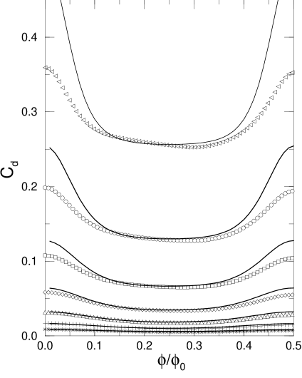
FIG. 2.: GOE to GUE transition for density of states correlations according to Eq. (15) (solid lines) and corresponding results from the numerical simulations of the Anderson model (symbols). The parameter $\lambda=1.21$ and $\epsilon=0.316$ ($\lhd$), $0.447$ ($\circ$), $0.631$ ($\Box$), $0.891$ ($\Diamond$), $1.26$ ($\bigtriangleup$), $1.78$ ($+$), $2.51$ ($\ast$).

FIG. 3.: Small $\epsilon$-behavior of $C_{d}$ with $W=2.4$. The solid line indicates $1/(2\pi^{2}\epsilon^{2})$, the long dashed line is $1/(4\pi^{2}\epsilon^{2})$ and the short dashed line denotes $1/(2\sqrt{\pi}\epsilon)$.

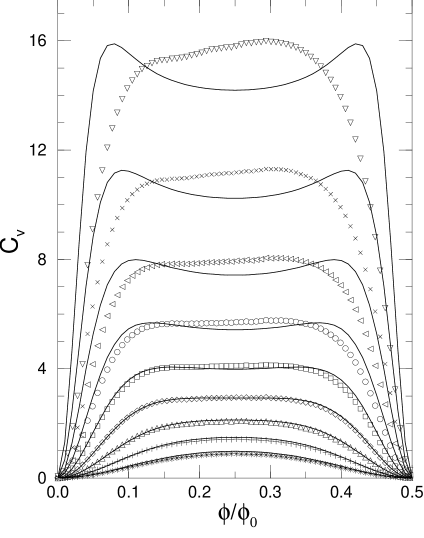
FIG. 4.: GOE to GUE transition for level velocity correlations according to Eq. (21) (solid lines) and corresponding results from the numerical simulations of the Anderson model (symbols). The parameters are the same as in Fig. 2. We additionally include the broadenings $\epsilon=0.158$ ($\bigtriangledown$) and $0.224$ ($\times$).

FIG. 5.: Determination of the parameter $\lambda$ from the small $\epsilon$-behavior of $C_{v}$ at $W=2.4$. By fitting the four first points ($\blacksquare$) on the left to Eq. (26) one gets a value $\lambda=1.22\pm 0.02$, whereas fitting the first eight points (bold $\square$) gives $\lambda=1.30\pm 0.01$. The difference between a plot of Eq. (26) with $\lambda=1.22$ (thin dashed line) and $\lambda=1.3$ (thin solid line) is very small.

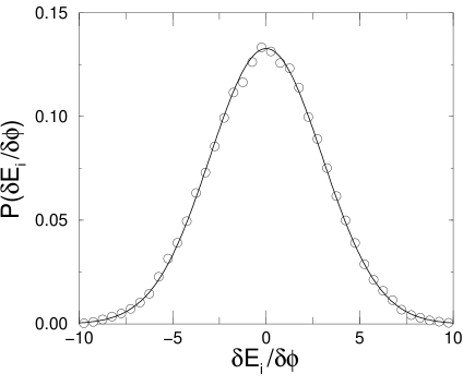
FIG. 6.: Distribution of level velocities averaged over flux values $\phi/\phi_{0}=0.175,\ldots,0.329$ and $90$ different realizations of disorder for $W=2.4$. The line represents a fit by a Gaussian distribution.

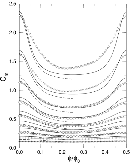
FIG. 7.: GOE to GUE transition for matrix element correlations according to Eq. (29) (solid lines) and corresponding results from the numerical simulations of the Anderson model (symbols). The parameters are the same as in Fig. 4 and the off-diagonal variance is taken to be $\sigma_{\rm off}^{2}=0.65$. The dashed lines indicate the $\nu=0$ term of Eq. (29) for small $\phi$.

FIG. 8.: Determination of the off-diagonal variance of the dipole moment operator by fitting the values of $C_{m}$ at small $\epsilon$ (filled symbols) to Eq. (33). The disorder is $W=2.4$.

FIG. 9.: Distribution for diagonal matrix elements of the dipole moment operator in units of the lattice constant and in case $W=2.4$, $\phi=0$ (filled circles) and averaged over all $\phi/\phi_{0}=0.175,...,0.329$ (open circles) with $\phi_{y}=0$. The lines are fits by Gaussian distributions. The variance $\sigma^{2}_{\mathrm{d}iag}=2\sigma^{2}_{\mathrm{o}ff}/\beta$ of the data is $1.3\pm 0.2$ for $\phi=0$ and $0.8\pm 0.1$ for $\phi/\phi_{0}=0.175,...,0.329$. The error limits represent the standard deviations of the values obtained for different realizations of disorder.

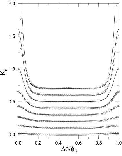
FIG. 10.: Parametric correlations of density of states according to Eq. (35) (solid lines) compared to the numerical results for the Anderson model (symbols) as a function of $\Delta\phi$. The parameters are $W=1.7$, $\lambda=2.5$ and $\epsilon=$ 0.112 ($\rhd$), 0.158 ($\bigtriangledown$), 0.224 ($\times$), 0.316 ($\lhd$), 0.447 ($\circ$), 0.631 ($\Box$), 0.891 ($\Diamond$), 1.26 ($\bigtriangleup$). The curves have been shifted by multiples of $0.1$ for clarity.

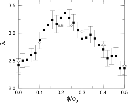
FIG. 11.: Parameter $\lambda=2{\cal D}/L^{2}$ for the Anderson model, determined by fitting Eq. (26) to the data ($\Diamond$) and from the variance of the level velocities ($\blacksquare$) with $W=1.7$ and different flux values in the presence of a transversal flux $\phi_{y}=\phi_{0}/4$.

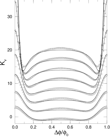
FIG. 12.: Parametric correlations of level velocities according to Eq. (38) (solid lines) compared to the numerical results for the Anderson model (symbols) as a function of $\Delta\phi$. The parameters are the same as in Fig. 10. The curves have been shifted by multiples of $1$ for clarity.

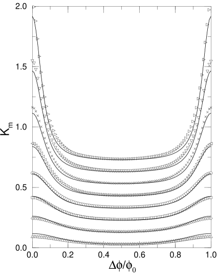
FIG. 13.: Parametric correlations of matrix elements according to Eq. (41) (solid lines) compared to the numerical results for the Anderson model (symbols) as a function of $\Delta\phi$. The parameters are the same as in Fig. 10 and $\sigma_{\mathrm{off}}^{2}=0.48$ has been used. The curves have been shifted by multiples of $0.1$ for clarity.

FIG. 14.: Distribution of real and imaginary parts of the off-diagonal dipole matrix elements at flux values $\phi=0$ (filled symbols) and $\phi=\phi_{0}/4$ (open symbols). Additionally, $\phi_{y}=0$ for $W=2.4$ ($\circ$) and $\phi_{y}=\phi_{0}/4$ for $W=1.7$ ($\diamond$). The lines represent fits by Gaussians. The distributions for $W=1.7$ have been shifted by $0.2$ for clarity.

- [1] Current address: Max-Planck-Institut für Physik komplexer Systeme, Nöthnitzer Str. 38, D-01187 Dresden, Germany
- [2] O. Bohigas, in Chaos and quantum physics, edited by M. J. Giannoni, A. Voros, and J. Zinn-Justin (North–Holland, Amsterdam, 1990), p. 87.
- [3] V. N. Prigodin et al., Phys. Rev. Lett. 75, 2392 (1995).
- [4] N. Taniguchi, A. V. Andreev, and B. L. Althshuler, Europhys. Lett. 29, 515 (1995).
- [5] B. Mehlig and N. Taniguchi, Phys. Rev. Lett. unpublished.
- [6] M. Wilkinson, J. Phys. A 22, 2795 (1989); E. J. Austin and M. Wilkinson, Nonlinearity 5, 1137 (1992); B. D. Simons and B. L. Altshuler, Phys. Rev. B 48, 5422 (1993).
- [7] E. P. Wigner, Proc. Camb. Phil. Soc. 47, 790 (1951); F. J. Dyson, J. Math. Phys. 3, 140 (1962); M. L. Mehta, Random Matrices, 2nd ed. (Academic Press, Boston, 1990); F. Haake, Quantum Signatures of Chaos, 2nd ed. (Springer, Berlin, 1992).
- [8] M. Wilkinson, J. Phys. A: Math. Gen. 21, 1173 (1988).
- [9] M. V. Berry and J. P. Keating, J. Phys. A: Math. Gen. 27, 6167 (1994).
- [10] M. Wilkinson and P. N. Walker, J. Phys. A: Math. Gen. 28, 6143 (1996).
- [11] J. Keating, unpublished.
- [12] B. Eckhardt et al., Phys. Rev. E. 52, 5893 (1995).
- [13] P. W. Anderson, Phys. Rev. 109, 1492 (1958).
- [14] B. Simons and B. L. Altshuler, Phys. Rev. Lett. 70, 4063 (1993);
- [15] E. Hofstetter and M. Schreiber, Phys. Rev. B. 48, 16979 (1993); ibid. 49, 14726 (1994); Phys. Rev. Lett. 73, 3137 (1994).
- [16] I. K. Zharekeshev and B. Kramer, Phys. Rev. Lett. 79, 717 (1997).
- [17] K. Müller, B. Mehlig, F. Milde, and M. Schreiber, Phys. Rev. Lett. 78, 215 (1997).
- [18] A. Pandey and M. L. Mehta, Commun. Math. Phys. 87, 447 (1983); J. Phys. A: Math. Gen. 16, 2655 (1983).
- [19] M. Wilkinson, J. Phys. A: Math. Gen. 22, 2795 (1989).
- [20] E. J. Austin and M. Wilkinson, Nonlinearity 5, 1137 (1992).
- [21] M. C. Gutzwiller, J. Math. Phys. 10, 1979 (1967).
- [22] B. Eckhardt, unpublished.
- [23] M. Berry, in Chaos and quantum physics, edited by M. J. Giannoni, A. Voros, and J. Zinn-Justin (North–Holland, Amsterdam, 1991), p. 251.
- [24] J. H. Hannay and A. M. O. de Almeida, J. Phys. A: Math. Gen. 17, 3429 (1984).
- [25] T. Dittrich, B. Mehlig, H. Schanz, and U. Similansky, Phys. Rev. E 57, 359 (1998)
- [26] J. Cullum and R. A. Willoughby, Lanczos Algorithms for Large Symmetric Eigenvalue Computations (Birkhäuser, Boston, 1985).
- [27] B. Kramer and A. MacKinnon, Rep. Prog. Phys. 56, 1469 (1993).
- [28] M. Schreiber and M. Ottomeier, J. Phys. Cond. Matter 4, 1959 (1992).
- [29] N. Dupuis and G. Montambaux, Phys. Rev. B. 43, 14390 (1991).
- [30] I. S. Gradshteyn and I. M. Ryzhik, Table of Integrals, Series, and Products (Academic Press, London, 1994).
- [31] O. Bohigas, M. J. Giannoni, A. M. O. de Almeida, and C. Schmit, Nonlinearity 8, 203 (1995).
- [32] E. Bogomolny and J. P. Keating, Phys. Rev. Lett. 77, 1472 (1996).
- [33] J. Keating, in: Quantum Chaos, edited by H. A. Cerdeira, M. C. Gutzwiller, R. Ramaswany and G. Casati (World Scientific, Singapore 1991).
- [34] M. Wilkinson, Phys. Rev. A. 41, 4645 (1991).
- [35] P. Walker, Ph.D. thesis, University of Strathclyde, Glasgow (1995).
- [36] In the infinite volume limit, the semiclassical estimate of for the dipole moment operator in a diffusive system diverges. Since we are dealing with a finite system here, the definition of is unproblematic in the present case.
- [37] V. Falko and K. B. Efetov, Phys. Rev. B 50, 11267 (1994).