Binary data corruption due to a Brownian agent

Abstract

We introduce a model of binary data corruption induced by a Brownian agent (active random walker) on a $d$-dimensional lattice. A continuum formulation allows the exact calculation of several quantities related to the density of corrupted bits $\rho$ ; for example the mean of $\rho$, and the density-density correlation function. Excellent agreement is found with the results from numerical simulations. We also calculate the probability distribution of $\rho$ in $d=1$, which is found to be log-normal, indicating that the system is governed by extreme fluctuations.

I Introduction

Brownian motion is one of the fundamental processes in Nature. Originally observed in the irregular motion of pollen grains by the botanist Brown[1], and cast into the language of the diffusion equation by Einstein[2], it has now been applied, in the mathematical framework of random walks[3], to an enormous variety of processes in the physical sciences and beyond. A very rich field of research has been built up around the behavior of a random walk coupled to a disordered environment[4], a good example being the anomalous diffusion of electrons in a disordered medium[5]. Also, one can consider a random walker being the disordering agent in its environment. Applications of the latter include the tagged diffusion of atoms in a crystal[6, 7, 8], or magnetic disordering due to a wandering vacancy[9].

In this paper we will introduce a particularly simple example of an active random walker (or Brownian agent) disordering its environment. Although the model is interesting in its own right, we believe it will have a useful application to the study of data corruption in ultra-small storage devices. Before pursuing this connection, we shall briefly describe the model (which will be more carefully defined in the next section). The two main features of the model are first, the Brownian agent (BA) performs a pure random walk – it is not affected by the environment in any way. Second, the environment is bistable. That is to say, it is composed of elements which may only exist in one of two possible states (see Ref.[10] for a loosely related random walk process). Thus we can consider the environment to be composed of binary data (our favored realization), magnetic spins, chemical species A and B, and so on. As the BA wanders through the environment it has a certain probability to switch the value of an element in its immediate vicinity. Thus, if we start with a system in which all elements exist in the same state (‘up’ say), and introduce the BA at the origin, then after some time, there will be a region around the origin in which the elements will be found in a mixture of ‘up’ and ‘down’ states. Naturally, the linear size of the region will grow on average as $\sqrt{t}$. The more subtle question concerns the degree of disordering which exists for elements within this region, and also their spatial correlations.. As we shall see, the statistics of the disordered elements are very rich. This is most convincingly demonstrated by the dominance of extreme fluctuations; for instance, the distribution of disordered elements is log-normal. Thus, typical and average events are quite distinct, and become ever more so as time proceeds.

Before giving an outline of the paper we shall say a few words about the potential relevance of this system to data corruption. With the advent of semiconductor memories (for dynamic random access memories (DRAM’s) and various types of read only memories (ROM’s)), there has been a tremendous drive within the semiconductor industry to produce ever-smaller memory devices[11, 12]. There are many properties (e.g. stability, power consumption, volatility, and cost) which must be balanced in the design of such devices. These factors determine the type of material used, and the geometry, dimension and architecture of the device. (For instance, three dimensional arrays have a very efficient address structure, and are stable against interference from bombarding alpha particles, but are very expensive to produce[11].) One of the main issues is the stability, or reliability, of the device. In semiconductor memories, there are many physical effects which can create hard errors (destruction or corruption of the device itself) or soft errors (corruption of the data stored in the device). In the latter category, the most common problems originate from electron clouds caused by alpha particles, but soft errors may also arise from electromigration and charge diffusion[13]. The key point is that different corruption mechanisms operate on different time scales (leading to the famous bath-tub curve of device reliability[12]). It is therefore important to know on what time-scales one should expect significant corruption from a given process. The model we propose here (namely data corruption via a BA) is probably not relevant for today’s semiconductor devices, since there are so many ‘mesoscopic’ processes occurring on the level of a flip-flop, that subtle correlations due to a BA will be washed out. However, we can look ahead to the new generation of (quantum) storage devices, in which a single electron (controlled in a gate via coulomb blockade) can store one bit of data. In this case, a microscopic BA may indeed play an important role in data corruption, and it will be necessary to understand its time-scales and efficacy of operation, so that we can minimize its influence. This paper constitutes a first step towards gaining such an understanding.

The outline of this paper is as follows. In the next section we shall carefully define the model (using discrete space and time) within the master equation formulation of stochastic processes. We shall derive some general statistical properties of the process, but we shall not enter into any explicit calculations. This is deferred to sections III-V in which we introduce a very simple continuum theory for the process, which is motivated by viewing the process as a stochastic cellular automaton. In section III we derive this continuum theory and, using the complementary descriptions of quantum mechanics (i.e. the Schrödinger equation and the Feynman path integral), we shall demonstrate its equivalence to the master equation formulation of section II. We then examine the case of one spatial dimension in section IV. The model is tractable, and a great deal of information may be derived concerning the mean density of disordered elements, their spatial correlations, and finally their entire distribution function. In section V, we briefly study higher dimensions, and derive some general statistical properties for the process, for an arbitrary spatial coupling between the BA and its environment. We also derive an expression for the mean density of disordered elements in two dimensions. In section VI we present results from extensive numerical simulations of the discrete process. In all cases, we find good agreement between the simulation results and the predictions of the continuum theory. We end the paper with a summary of the work, and some ideas for future study.

II Discrete formulation of the model

We consider binary data bits on a $d$-dimensional hypercubic lattice. For convenience we shall represent each bit by an Ising spin $\sigma_{\bf r}$ , where the index ${\bf r}$ represents a discrete lattice vector. The spin takes the value $+1(-1)$ for a data bit which is uncorrupted (corrupted). Thus, the initial configuration is a lattice of spins, all of which take the value $+1$. [We prefer to describe the system almost exclusively in terms of the spin variables. Thus we shall use phrases such as ‘magnetization density’, or ‘global magnetization’. The translation of these quantities to the corresponding properties for corrupted data bits is immediate as one only need replace $\sigma_{\bf r}$ by $(1-2n_{\bf r})$, where $n_{\bf r}$ denotes the presence (with value unity) or absence (with value zero) of a corrupted bit. Similarly, we shall often refer to the average magnetization density $m$ , which is related to the average density of corrupted bits ${\bar{\rho}}$ via $m=1-2{\bar{\rho}}$ .] We denote the position of the BA by the lattice vector ${\bf R}$. Each time step, the BA has a probability $p$ to make a jump to one of its ($2d$) nearest neighbors. For the sake of generality, we will not insist that the BA always flips a spin (i.e. changes a data bit) as it moves. Thus, on a given jump, we allow the BA to flip the spin at the site it is leaving, with a probability $q$. In this section we shall describe the process via a master equation[14]. Namely, we shall define the dynamics through the evolution of the distribution $P({\bf R},\{\sigma_{\bf r}\},t)$, which is the probability that at time $t$ the BA is at position ${\bf R}$, and the spins have configuration $\{\sigma_{\bf r}\}$. Given the above rules, the master equation takes the form

$$P({\bf R},\{\sigma_{\bf r}\},t+\delta t)=(1-p)P({\bf R},\{\sigma_{\bf r}\},t) + {p(1-q)\over 2d}\sum\limits_{\bf l}P({\bf R}+{\bf l},\{\sigma_{\bf r}\},t)$$ (1)

$$+ {pq\over 2d}\sum\limits_{\bf l}P({\bf R}+{\bf l},\cdots,-\sigma_{{\bf R}+{\bf l}},\cdots,t)\ ,$$ (2)

where $\{{\bf l}\}$ represent the $2d$ orthogonal lattice vectors (which have magnitude $l$).

The natural quantities to extract from the distribution $P$ are conditional averages. The simplest is the mean value of the spin at position ${\bf r}_{1}$ at time $t$, given the BA is at position ${\bf R}$. This is defined via

$$\Theta({{\bf r}_{1}},t\ |\ {\bf R})\equiv{\rm Tr}_{\sigma}\ \sigma_{{\bf r}_{1}}\ P({\bf R},\{\sigma_{\bf r}\},t)\ .$$ (3)

Higher order conditional averages may be defined accordingly. Performing the spin trace over the master equation with a weight of $\sigma_{\bf r}$ yields

$$\Theta({\bf r},t+\delta t\ |\ {\bf R})-\Theta({\bf r},t\ |\ {\bf R}) = {p\over 2d}\sum\limits_{\bf l}\bigl{[}\Theta({\bf r},t\ |\ {\bf R}+{\bf l})-\Theta({\bf r},t\ |\ {\bf R})\bigr{]}$$ (4)

$$- {pq\over d}\ \Theta({\bf r},t\ |\ {\bf r})\sum\limits_{\bf l}\delta_{{\bf r},{\bf R}+{\bf l}}\ .$$ (5)

The above equation has a physically appealing form. The rate of change of $\Theta$ has two contributions. The first is lattice diffusion, as given by the first sum on the r.h.s. The second contribution vanishes unless the spin in question is in the immediate vicinity of the BA, in which case it acts as a sink.

At this point in the discussion it is worthwhile to consider the continuum limit. Namely we take the time scale $\delta t$ and the lattice scale $l$ to zero, and define a diffusion constant $D\equiv l^{2}p/\delta t$. We also introduce a coupling $\lambda\propto ql/\delta t$. Then replacing the Kronecker $\delta$-function in Eq.(4) by a Dirac $\delta$-function we find

$$\partial_{t}\Theta({\bf r},t\ |\ {\bf R})=D\nabla_{\bf R}^{2}\Theta({\bf r},t\ |\ {\bf R})-\lambda\ \Theta({\bf r},t\ |\ {\bf r})\delta^{d}({\bf r}-{\bf R})\ .$$ (6)

It is important to note that this continuum equation is not strictly derived from Eq.(4), as we have not proved that the continuum limit exists. In fact, we shall find that for $d\geq 2$, the lattice scale $l$ is crucial, and consequently we must soften the Dirac $\delta$-function to a function $\Delta_{l}({\bf r})$ which is sharply peaked (over a linear scale $l$) with unit integral over ${\cal R}^{d}$. One actually expects this to be the case, as Eq.(6) is the imaginary-time Schrödinger equation for a particle under the influence of a repulsive $\delta$-function potential. [Note the independent spatial variable in this quantum system is ${\bf R}$, with the variable ${\bf r}$ simply labelling the position of the potential.] It is well known[15] that the repulsive $\delta$-function potential is ‘invisible’ to the particle for $d\geq 2$, and one usually cures this by smearing the potential just as described above. The quantum mechanics analogy will prove useful in the next section when we construct an alternative continuum model.

Before leaving this section we shall indicate the derivation of a non-trivial statistical relation hidden inside Eq.(4). First, we must define the initial condition. As mentioned before, given that up-spins denote uncorrupted data, the initial value of each spin is $+1$. There is a slight subtlety of definition regarding the value of the spin at the site where the BA is initially planted. (This position shall be taken to be the origin, without any loss of generality.) We shall take this spin to be initially $-1$ so that immediately after the BA has moved away the spin at the origin has value $+1$. Thus we have

$$P({\bf R},\{\sigma_{\bf r}\},0)=\delta_{{\bf R},{\bf 0}}\delta_{\sigma_{\bf 0},-1}\prod\limits_{{\bf r}\neq{\bf 0}}\delta_{\sigma_{\bf r},1}\ ,$$ (7)

and consequently,

$$\Theta({\bf r},0\ |\ {\bf R})=\delta_{{\bf R},{\bf 0}}(1-2\delta_{{\bf r},{\bf 0}})\ .$$ (8)

We may obtain the following two averages from $\Theta({\bf r},t\ |\ {\bf R})$. The first is the average value of the spin at the origin. This is simply given by $m_{\bf 0}(t)=\sum_{\bf R}\Theta({\bf 0},t\ |\ {\bf R})$. The second average is the quantity $\sum_{\bf R}\Theta({\bf R},t\ |\ {\bf R})$, which corresponds to averaging the value of the spin at the site where the BA happens to be at time $t$. One can prove that

$$\sum\limits_{\bf R}\Theta({\bf 0},t\ |\ {\bf R})=\sum\limits_{\bf R}\Theta({\bf R},t\ |\ {\bf R})\ ,$$ (9)

for all $t$. We arrive at the above result by essentially solving the partial difference equation (4) using discrete Fourier and Laplace transforms. The details can be found in Appendix A.

This result is useful for proving a more physically relevant relation. Let us denote the average global magnetization by

$$M(t)=\sum\limits_{\bf R}\sum\limits_{\bf r}[\Theta({\bf r},0\ |\ {\bf R})-\Theta({\bf r},t\ |\ {\bf R})]\ ,$$ (10)

where we have defined it relative to the (infinite) initial magnetization. This quantity essentially measures the average of the total number of corrupted bits (up to a factor of 2). Summing Eq.(4) over ${\bf r}$ and ${\bf R}$ gives

$$M(t+\delta t)-M(t)=2pq\sum\limits_{\bf r}\Theta({\bf r},t\ |\ {\bf r})\ .$$ (11)

Then using (9) we can rewrite the above relation in the form

$$M(t+\delta t)-M(t)=2pq\sum\limits_{\bf R}\Theta({\bf 0},t\ |\ {\bf R})=2pq\ m_{\bf 0}(t)\ .$$ (12)

In other words, the rate of change of the mean global magnetization is proportional to the mean magnetization density at the origin. This is a non-trivial relation between a global and a local quantity.

In principle, one can obtain exact results for many interesting quantities (like the mean magnetization density, or correlation functions) by directly solving for the conditional averages, as illustrated in Appendix A. However, we prefer to obtain results from a continuum theory; partly because the calculations are a little easier, but more importantly because we can access more sophisticated properties of the system, such as the probability distribution of the coarse-grained magnetization density.

III Continuum theory

In this section we shall motivate a particularly simple continuum description of the data corruption process, and show its equivalence to the discrete theory of the previous section.

There is an alternative method of characterizing the evolution of the system, other than using the evolution of the probability distribution $P({\bf R},\{\sigma_{\bf r}\},t)$ via the master equation. This method consists of writing the local rules for the process in the spirit of a stochastic cellular automaton (SCA)[16]. Let us focus on the case that at each time step the BA makes a random jump to one of its nearest neighbors, and that the spin at the site which it leaves behind, definitely flips. This corresponds to setting $p=q=1$. The local rules for such a process are easily written down. Let us denote the time-dependent position of the BA by ${\bf R}(t)$, a randomly chosen unit lattice vector by ${\bf l}(t)$, and the time-dependent value of the spin at site ${\bf r}$ by $\sigma_{\bf r}(t)$. Then we have

$${\bf R}(t+\delta t) = {\bf R}(t)+{\bf l}(t)$$ (13)

$$\sigma_{\bf r}(t+\delta t) = \sigma_{\bf r}(t)(1-2\delta_{{\bf r},{\bf R}(t)})$$ (14)

We are interested in a continuum limit of these two rules. The first is nothing more than a random walk. We take the lattice vector ${\bf R}(t)$ to be a continuum vector (i.e. each of the $d$ components is a real number), and we replace the random unit lattice vector ${\bf l}(t)$ by a continuum vector ${\bf{\xi}}(t)$, each component of which is a uncorrelated Gaussian random variable with zero mean (i.e. $\xi_{i}(t)$ is a white noise process). The correlator of ${\bf{\xi}}$ is given by

$$\langle\xi_{i}(t)\xi_{j}(t^{\prime})\rangle=D^{\prime}\delta_{i,j}\delta(t-t^{\prime})\ ,$$ (15)

where here and henceforth, angled brackets indicate an average over the noise (or equivalently the paths of the BA). Then, on taking $\delta t\rightarrow 0$, Eq.(13) assumes the form

$${d{\bf R}\over dt}={\bf{\xi}}(t)\ ,$$ (16)

which is the familiar equation for a continuum random walker where $D^{\prime}$ is the diffusion constant[14]. The second SCA rule is more complicated to generalize to the continuum. As a first step let us define a coarse-grained magnetization density $\phi({\bf r},t)$ in the following way. We imagine defining a large region around the lattice site ${\bf r}$ and summing all the spins in that region. Their sum (suitably normalized) constitutes $\phi({\bf r},t)$, with the label ${\bf r}$ denoting a point in the ${\cal R}^{d}$ continuum. An entirely analogous procedure is used in motivating the Landau-Wilson free energy functional from the Ising model of ferromagnetism[17]. The difficulty in our case is that we cannot derive a closed equation for $\phi$ from the discrete rule (14). We therefore make the following approximation. Splitting the r.h.s. of (14) into two pieces, we see that the first may be taken over to the l.h.s. which may then be taken to be a time derivative in the limit of $\delta t\rightarrow 0$ . The second piece resembles a decay term centered at ${\bf r}={\bf R}$. So, we postulate that the coarse-grained magnetization density satisfies

$$\partial_{t}\phi({\bf r},t)=-\lambda^{\prime}\phi({\bf r},t)\delta^{d}({\bf r}-{\bf R}(t))\ ,$$ (17)

where $\lambda^{\prime}$ is a phenomenological parameter which describes how strongly the magnetization density is coupled to the BA. We stress that the field $\phi({\bf r},t)$ is a function of the continuous space and time variables ${\bf r}$ and $t$, and a functional of the path ${\bf R}(t)$ of the BA.

Now, the above heuristic derivation of the continuum theory was based on a SCA for the case in which the BA always moves ($p=1$), and for which the spin located at the previous BA position is always flipped ($q=1$). In general $p$ and $q$ are both less than unity. Intuitively we expect a very simple renormalization of our phenomenological parameters as $p$ and $q$ are changed. The diffusion constant $D^{\prime}$ should be proportional to $p$, and the strength of the spin-BA coupling $\lambda^{\prime}$ should be proportional to both $p$ and, more importantly, $q$. Thus we see a very close correspondence between $D^{\prime}$ and $\lambda^{\prime}$ in the current continuum theory, and the parameters $D$ and $\lambda$ which were introduced in the continuum limit (6) of the discrete equation (4). In fact they are identical, as will emerge in the following discussion.

One of the positive features of the continuum theory as described by (17) is that one may immediately integrate the equation to find the magnetization density as an explicit functional of the path of the BA. As an initial condition we take $\phi({\bf r},0)=1$ for all ${\bf r}$. The subtlety encountered in the discrete theory concerning the initial value of the spin at the origin disappears here since the coarse grained function $\phi$ is not sensitive to the value of one inverted spin. Straightforward integration of (17) yields

$$\phi({\bf r},t)=\exp\left[-\lambda^{\prime}\int\limits_{0}^{t}dt^{\prime}\ \delta^{d}({\bf r}-{\bf R}(t^{\prime}))\right]\ .$$ (18)

It is important to note at this stage that the magnetization density $\phi$ is clearly positive for all ${\bf r}$ and $t$. Therefore within our continuum formulation, we have ignored paths of the BA which create large patches containing a majority of down spins (i.e. corrupted bits). Such patches will occur, but their frequency of occurrence is certainly very small since the system starts in a completely uncorrupted state. For instance, the probability for the BA to create a purely negative domain of $N$ spins is of the order $e^{-N}$. Therefore, so long as we coarse-grain the original spin model over a sufficiently large scale, we can be confident that the most important configurations have been retained in the continuum theory. Ultimately, one must justify such an approximation a posteriori by comparison with either results from the discrete theory, or from numerical simulations. As we shall see, both of these support the current continuum model and the approximations contained therein.

We shall now connect the continuum theory as given by (18), and the continuum limit (6) of the discrete theory, as given by (4). The mean magnetization density in the discrete theory is given by

$$m_{\bf r}(t)=\sum\limits_{\bf R}\Theta({\bf r},t\ |{\bf R}){{\rm CL}\atop\longrightarrow}\int d^{d}R\ \Theta({\bf r},t\ |{\bf R})$$ (19)

where in the continuum limit, we have replaced the sum over BA positions by an integral, and the field $\Theta$ satisfies the imaginary-time Schrödinger equation as given in (6). In the alternative continuum theory, we can find the mean magnetization density by averaging the coarse-grained density $\phi({\bf r},t)$ over all paths ${\bf R}(t)$. Each path is weighted by a Gaussian factor

$${\cal N}{\rm exp}\left\{-{1\over 2D^{\prime}}\int\limits_{0}^{t}dt^{\prime}\ {\bf{\xi}}(t^{\prime})^{2}\right\}={\cal N}{\rm exp}\left\{-{1\over 2D^{\prime}}\int\limits_{0}^{t}dt^{\prime}\ \left({d{\bf R}\over dt^{\prime}}\right)^{2}\right\}\ ,$$ (20)

where ${\cal N}$ is a normalization factor. Therefore we can write the average of $\phi$ as a functional integral

$$m({\bf r},t)=\langle\phi({\bf r},t)\rangle = {\cal N}\int{\cal D}{\bf R}(t^{\prime})\ {\rm exp}\left\{-{1\over 2D^{\prime}}\int\limits_{0}^{t}dt^{\prime}\ \left({d{\bf R}\over dt^{\prime}}\right)^{2}\right\}\ \phi({\bf r},t)\ ,$$ (21)

$$= {\cal N}\int{\cal D}{\bf R}(t^{\prime})\ {\rm exp}\left\{-\int\limits_{0}^{t}dt^{\prime}\ \left[{1\over 2D^{\prime}}\left({d{\bf R}\over dt^{\prime}}\right)^{2}+\lambda^{\prime}\delta^{d}({\bf r}-{\bf R}(t^{\prime}))\right]\right\}\ ,$$ (22)

$$= {\cal N}\int d^{d}R_{f}\int\limits^{{\bf R}_{f}}{\cal D}{\bf R}(t^{\prime})\ {\rm exp}\left\{-\int\limits_{0}^{t}dt^{\prime}\ \left[{1\over 2D^{\prime}}\left({d{\bf R}\over dt^{\prime}}\right)^{2}+\lambda^{\prime}\delta^{d}({\bf r}-{\bf R}(t^{\prime}))\right]\right\}\ ,$$ (23)

where we have used (18) in going from the first line to the second, and we have introduced the final position of the BA (i.e. R(t)) as a free integration variable ${\bf R}_{f}$ in rewriting the second line as the third. The reason for this cosmetic change is to make explicit the fact that $\langle\phi({\bf r},t)\rangle$ can be expressed as a spatial integral over the final BA position, where the integrand is itself a path integral over BA trajectories. This path integral is nothing more than a re-expression of the solution of an imaginary time Schrödinger equation (using the well-known Feynman path integral formulation of quantum mechanics[18]) for a particle in a repulsive $\delta$-function potential. We can now see the connection: Eq. (21) is an exact restatement of Eqs. (6) and (19), with the identification $D^{\prime}=D$ and $\lambda^{\prime}=\lambda$. [So, henceforth we shall drop the primes in the material parameters.] To summarize, by utilizing the complementary formulations of quantum mechanics via the Schrödinger equation and the Feynman path integral, we have shown that the continuum limit of the master equation is identical to the continuum theory constructed at the beginning of this section.

Two final points are in order. First, as noted in the previous section, the $\delta$-function potential must be replaced by a smeared function $\Delta_{l}({\bf r})$ for $d\geq 2$; thus in our continuum theory encapsulated in Eq.(17), we shall make a similar replacement when studying two or higher dimensions. Second, we have established a connection between the master equation and Eq.(17) only at the level of the first moment. It is straightforward to extend each formulation to higher order correlation functions, and indeed one finds an exact correspondence. For instance, we can define the conditional spin-spin correlation function within the discrete theory

$$\Theta({{\bf r}_{1}},{{\bf r}_{2}},t\ |\ {\bf R})\equiv{\rm Tr}_{\sigma}\ \sigma_{{\bf r}_{1}}\sigma_{{\bf r}_{2}}\ P({\bf R},\{\sigma_{\bf r}\},t)\ .$$ (24)

Using the master equation one can show that in the continuum limit this function satisfies the Schrödinger equation for a particle under the influence of two repulsive $\delta$-function potentials located at ${\bf r}_{1}$ and ${\bf r}_{2}$. Similarly, we can construct the coarse-grained two-point correlation function from Eq.(18) by evaluating $\langle\phi({\bf r}_{1},t)\phi({\bf r}_{2},t)\rangle$. It is easy to see that this quantity is given by an integral over the analogous path-integral for two repulsive $\delta$-function potentials.

Having completed our formulation of a simple continuum theory, and shown its equivalence to the continuum limit of the master equation, we shall proceed to the next section in which we present a comprehensive solution of the model in one dimension.

IV Results in one dimension

In this section we restrict ourselves to one dimension. This does not necessarily mean a single chain of sites. Rather, we shall exclusively study the continuum theory of the last section, and in this case, for large enough times, $d=1$ refers to any system which has an infinite longitudinal dimension, and finite transverse dimensions (for instance an infinitely long strip). This is the case, since as time proceeds, the correlation length will eventually become greater than the transverse size of the system, thereby only allowing the longitudinal fluctuations to continue growing, as is the case in a strictly one-dimensional system.

The continuum model described in the previous section can be viewed as a ‘non-conserved’ cousin of the continuum theory of vacancy mediated diffusion (a process which in the spin language conserves magnetization) introduced recently[8]. An exact analysis of the latter theory was possible using infinite order perturbation theory in the spin-BA coupling $\lambda$. We shall use the same technique here, as it leads rather directly to a full solution. Alternatively, one may solve the Schrödinger equation for the conditional averages. However, there are some important quantities (like the distribution of the magnetization density) which cannot be easily recovered from the latter approach.

Our starting point is the integrated solution of the continuum formulation as given in Eq.(18). First, we shall derive an expression for the magnetization density $m(x,t)$. Performing a direct average of Eq.(18) and expanding in powers of $\lambda\ (=\lambda^{\prime})$, we have

$$m(x,t)=\langle\phi(x,t)\rangle=\sum\limits_{n=0}^{\infty}(-\lambda)^{n}\chi_{n}(x,t)\ ,$$ (25)

where $\chi_{0}(x,t)=1$, and for $n>0$

$$\chi_{n}(x,t)={1\over n!}\left\langle\left[\int\limits_{0}^{t}d\tau\ \delta(x-R(\tau))\right]^{n}\right\rangle\ .$$ (26)

We refer the reader to Appendix B in which the above average is explicitly calculated. The result is

$$\chi_{n}(x,t)=\int\limits_{0}^{t}d\tau_{1}\int\limits_{0}^{\tau_{1}}d\tau_{2}\cdots\int\limits_{0}^{\tau_{n-1}}d\tau_{n}\ g(0,\tau_{1}-\tau_{2})\cdots g(0,\tau_{n-1}-\tau_{n})g(x,\tau_{n})\ ,$$ (27)

where $g(x,t)=(2\pi Dt)^{-1/2}\exp(-x^{2}/2Dt)$ is the probability density of the BA.

The structure of Eq.(27) is that of an $n$-fold convolution, so we may utilize a Laplace transform to good effect. We have (for $n>0$)

$${\hat{\chi}}_{n}(x,s)\equiv\int\limits_{0}^{\infty}dt\ e^{-st}\ \chi_{n}(x,t)={1\over s}\ {\hat{g}}(0,s)^{n-1}{\hat{g}}(x,s)\ .$$ (28)

Performing the sum over these functions as dictated by Eq.(25) we find

$${\hat{m}}(x,s)={1\over s}\left[1-{\lambda{\hat{g}}(x,s)\over 1+\lambda{\hat{g}}(0,s)}\right]\ .$$ (29)

We note in passing that a similar result is easily derived for any $d\in(0,2)$. The case of $d\geq 2$ is more complicated as the function $g(0,t)$ is no longer integrable.

This expression for the Laplace transform of $m$ is exact. This will prove to be important when we come to evaluate the distribution function of ${\cal P}(m)$. The inverse of the Laplace transform is given by

$$m(x,t)={\rm erf}\left[{|x|\over(2Dt)^{1/2}}\right]+\exp\left({\lambda|x|\over D}+{\lambda^{2}t\over 2D}\right)\ {\rm erfc}\left[\lambda\left({t\over 2D}\right)^{1/2}+{|x|\over(2Dt)^{1/2}}\right]\ ,$$ (30)

where ${\rm erf}(z)$ and ${\rm erfc}(z)$ are error functions[19]. Considering the long time behavior of the above expression, we have for $x=0$

$$m(0,t)=\left({2D\over\pi\lambda^{2}t}\right)^{1/2}\left[1+O\left({D\over\lambda^{2}t}\right)\right]\ .$$ (31)

One can also retrieve the spatial behavior with little effort. For small $x$ we have

$$m(x,t)=m(0,t)+\left({2x^{2}\over\pi Dt}\right)^{1/2}+\cdots\ \ \ \ ,\ x\ll(Dt)^{1/2}\ .$$ (32)

The large $x$ behavior has two regimes:

$$m(x,t) = 1-\left({2Dt\over\pi x^{2}}\right)^{1/2}\exp\left({-x^{2}\over 2Dt}\right)+\cdots\ \ \ \ ,(Dt)^{1/2}\ll x\ll\lambda t$$ (33)

$$m(x,t) = 1-\left({\lambda t\over|x|}\right)\left({2Dt\over\pi x^{2}}\right)^{1/2}\exp\left({-x^{2}\over 2Dt}\right)+\cdots\ \ \ \ ,x\gg\lambda t\ .$$ (34)

It is interesting to note that apart from the natural diffusion scale $(Dt)^{1/2}$, there is a larger ‘ballistic’ scale $\lambda t$ in the system, beyond which the disordering efficacy of the BA is much reduced, since it makes so few visits to these distant sites. There is no simple (ı.e. single length) scaling form for $m(x,t)$.

Next we consider the continuum analogues of Eqs.(9)-(12). We define the average global magnetization (relative to its initial value) as

$$M(t)=\int\limits_{-\infty}^{\infty}dx\ \left[\langle\phi(x,0)\rangle-\langle\phi(x,t)\rangle\right]\ ,$$ (35)

which may be compared to the discrete version in Eq.(10). Integrating and averaging the continuum model (17) yields

$${dM(t)\over dt}=\lambda\langle\phi(R(t),t)\rangle\ ,$$ (36)

which is to be compared with Eq.(11). This last equation indicates that we may explicitly find an expression for $\langle\phi(R(t),t)\rangle$ by calculating the time derivative of the spatial integral of $m(x,t)=\langle\phi(x,t)\rangle$. This may be done at the level of the perturbation series (25), from which one may show that the following relation holds exactly, for all times:

$$m(0,t)=\langle\phi(R(t),t)\rangle\ ,$$ (37)

which is the continuum analogue of Eq.(9). Finally, combining Eqs.(36) and (37) we have

$${dM(t)\over dt}=\lambda m(0,t)\ .$$ (38)

Thus, the non-trivial relation between the rate of change of the global magnetization, and the mean of the magnetization density at the origin, is seen to be exact within the continuum model (which complements the exact relation $(\ref{glomag3})$ found in the discrete framework). Similar results are easily obtained for all $d\in(0,2)$. In section V we shall derive a slightly more complicated form of $(\ref{glomagc3})$ (involving the smearing function $\Delta_{l}$) which is appropriate for higher dimensional systems. Directly from Eqs.(31) and (38) we note that $M(t)\sim\sqrt{t}$ ; thus, the average number of corrupted bits in $d=1$ increases as the square root of time.

We now turn to spatial correlations in the system. These are most easily probed via the two-point correlation function

$$C(x,t) = \langle\phi(x,t)\phi(0,t)\rangle$$ (39)

$$= \left\langle\exp\left(-\lambda\int\limits_{0}^{t}dt^{\prime}\ \bigl{[}\delta(x-R(t^{\prime}))+\delta(R(t^{\prime}))\bigr{]}\right)\right\rangle\ ,$$ (41)

where we have used the solution (18) in the second line. This average can be calculated using infinite order perturbation theory in $\lambda$, just as was used to evaluate $m(x,t)$. We write

$$C(x,t)=\sum\limits_{n=0}^{\infty}(-\lambda)^{n}c_{n}(x,t)\ ,$$ (42)

with $c_{0}=1$. For $n>0$, a given term $c_{n}$ can be explicitly evaluated by making integral representations of the $n$ $\delta$-functions, and performing the average over the paths $R(t)$ (as described in Appendix B). Thus one has

$$c_{n}(x,t)=\int\limits_{0}^{t}d\tau_{1}\int\limits_{0}^{\tau_{1}}d\tau_{2}\cdots\int\limits_{0}^{\tau_{n-1}}d\tau_{n} \int{dk_{1}\over 2\pi}\ (1+e^{-ik_{1}x})\cdots\int{dk_{n}\over 2\pi}\ (1+e^{-ik_{n}x})$$ (43)

$$\times \exp\left[-{D\over 2}\sum\limits_{m=1}^{n}\left(\sum\limits_{l=1}^{m}k_{l}^{2}\right)(\tau_{m}-\tau_{m+1})\right]\ ,$$ (44)

with the notation $\tau_{n+1}\equiv 0$. This $2n$-fold integral can be reduced using Laplace transform in time, such that the integrals over $\{k_{i}\}$ may be performed, as described in Appendix C. The result is

$${\hat{c}}_{n}(x,s)={1\over s(2sD)^{n/2}}\left(1+\exp\left[-\left({2s\over D}\right)^{1/2}|x|\right]\right)^{n}\ .$$ (45)

Summing over these functions with a weight of $(-\lambda)^{n}$ and inverting the Laplace transform using a Bromwich integral[20], we have

$$C(x,t)=\int_{\gamma}{ds\over 2\pi i}\ {\exp(s{\tilde{t}})\over s^{1/2}[1+s^{1/2}+\exp(-s^{1/2}|{\tilde{x}}|)]}\ ,$$ (46)

where, as usual, the contour $\gamma$ is parallel to the imaginary axis, and to the right of any singularities. We have rescaled space and time as ${\tilde{x}}=x\lambda/D$ and ${\tilde{t}}=t\lambda^{2}/2D$.

This integral may be evaluated for large ${\tilde{t}}$ in the following way. We re-express the integral as an expansion in powers of $\exp(-s^{1/2}|{\tilde{x}}|)$ (which is not the same as our original expansion in powers of $\lambda$). So we have

$$C(x,t)=\sum_{n=0}^{\infty}(-1)^{n}I_{n}({\tilde{x}},{\tilde{t}})\ ,$$ (47)

with

$$I_{n} = \int_{\gamma}{ds\over 2\pi i}\ \ {e^{s{\tilde{t}}-ns^{1/2}|{\tilde{x}}|}\over s^{1/2}(1+s^{1/2})^{n+1}}$$ (48)

$$= {1\over 2\pi}\int\limits_{0}^{\infty}du\ {e^{-u{\tilde{t}}}\over u^{1/2}}\ \left[{e^{-inu^{1/2}|{\tilde{x}}|}\over(1+iu^{1/2})^{n}}+{e^{inu^{1/2}|{\tilde{x}}|}\over(1-iu^{1/2})^{n}}\right]\ ,$$ (50)

where the second line is the explicit form of the integral after integrating around the only singularity – a branch point located at $s=0$. The integral over $u$ may be simplified for ${\tilde{t}}\gg 1$ to give

$$I_{n} \simeq {1\over\pi{\tilde{t}}^{1/2}}\int\limits_{0}^{\infty}du\ {e^{-u}\over u^{1/2}}\cos\left({nu^{1/2}|{\tilde{x}}|\over{\tilde{t}}^{1/2}}\right)$$ (51)

$$= {1\over(\pi{\tilde{t}})^{1/2}}\exp\left(-{n^{2}{\tilde{x}}^{2}\over 4{\tilde{t}}}\right)\ .$$ (52)

In these rescaled units, we have from Eq.(31) $m(0,{\tilde{t}})\simeq(\pi{\tilde{t}})^{-1/2}$ (for large ${\tilde{t}}$). Thus, we may resum the functions $\{I_{n}\}$ to find

$${C(x,t)\over m(0,t)}\ \simeq \ \sum\limits_{n=0}^{\infty}(-1)^{n}\exp\left(-{n^{2}{\tilde{x}}^{2}\over 4{\tilde{t}}}\right)$$ (53)

$$= \ {1\over 2}\left[1+\theta_{4}\left(0,\exp(-x^{2}/2Dt)\right)\right]\ ,$$ (55)

where $\theta_{4}(q,z)$ is a Jacobi theta function (with norm $q$)[19]. Note, we have written the last line in unscaled variables, and we see that the ratio of the correlation function to $m(0,t)$ does not depend on $\lambda$ for large times. The behavior of $C(x,t)$ in the limits of large and small $x$ are as follows. For large $x$, the fields at the origin and at $x$ will be uncorrelated, so that $C(x,t)\simeq m(0,t)m(x,t)\simeq m(0,t)$, the latter result following since $m(x,t)\simeq 1$ for $x\gg\sqrt{t}$. At the other extreme, as $x\rightarrow 0$, $C(x,t)\rightarrow\langle\phi(0,t)^{2}\rangle$. Referring to the exact solution of the continuum model, Eq.(18), one can see that the second moment of the magnetization density is actually given exactly by $m(0,t;2\lambda)$ (where the last (optional) argument indicates the parametric dependence on the spin-BA coupling). So for long times we take the expression for $m(0,t;\lambda)$ given in Eq.(31) and replace $\lambda$ by $2\lambda$. Therefore $\langle\phi(0,t)^{2}\rangle\simeq m(0,t;\lambda)/2$ for ${\tilde{t}}\gg 1$. Thus, the limits of the function $C(x,t)/m(0,t)$ are 1/2 (for small $x$) and unity (for large $x$), which is naturally consistent with the analytic form given above in terms of the Jacobi theta function. In section VI we shall compare this expression with results from a numerical simulation of the discrete model described earlier.

To complete our study of the properties of this system in one dimension, we shall consider the complete probability distribution ${\cal P}(\phi,x,t)$ of the magnetization density. We shall be able to calculate this exactly, since i) we can see from (18) that the $n^{\rm th}$ moment of the density is related to the mean density with a replacement $\lambda\rightarrow n\lambda$; and ii) we have an exact expression for the mean density (albeit in the Laplace transform variable $s$). The first point is a fortuitous property of our continuum model which we should certainly exploit. The second property is less obvious. One might imagine that, given we know all density moments via the first, even the asymptotic form for the mean density would be sufficient to calculate the probability distribution (for large times). This is not the case as we shall see – the complete analytic structure of $m(x,t;\lambda)$ is required in order to reconstruct the distribution ${\cal P}$.

We define ${\cal P}$ via

$${\cal P}(\phi,x,t)=\langle\delta(\phi-\phi_{R}(x,t))\rangle\ ,$$ (56)

where $\phi_{R}(x,t)$ is the stochastic field solution given in Eq. (18). We can re-express the $\delta$-function using a frequency integral, and expand in powers of the field as follows:

$${\cal P}(\phi,x,t) = \int\limits_{-\infty}^{\infty}{d\omega\over 2\pi}\ e^{-i\omega\phi}\ \langle\exp\left[i\omega\phi_{R}(x,t)\right]\rangle$$ (57)

$$= \int\limits_{-\infty}^{\infty}{d\omega\over 2\pi}\ e^{-i\omega\phi}\ \sum\limits_{n=0}^{\infty}{(i\omega)^{n}\over n!}\langle\phi_{R}(x,t)^{n}\rangle$$ (58)

$$= \int\limits_{-\infty}^{\infty}{d\omega\over 2\pi}\ e^{-i\omega\phi}\ \sum\limits_{n=0}^{\infty}{(i\omega)^{n}\over n!}m(x,t;n\lambda)\ ,$$ (59)

the last line following from the property i) alluded to above.

So the Laplace transform (over time) of ${\cal P}$ is given in terms of the Laplace transform of $m(x,t;n\lambda)$. From Eq.(29) we have

$${\hat{m}}(x,s;n\lambda) = {1\over s}\left[1-{n\lambda{\hat{g}}(x,s)\over 1+n\lambda{\hat{g}}(o,s)}\right]$$ (60)

$$= {{\hat{g}}(0,s)-{\hat{g}}(x,s)\over s{\hat{g}}(0,s)}\ +\ {{\hat{g}}(x,s)\over s{\hat{g}}(0,s)(1+n\lambda{\hat{g}}(0,s))}\ ,$$ (62)

where the second line follows from some algebraic manipulations. The first term is easily handled as it is independent of $n$. Thus the sum over $n$ for this term (as is required in Eq.(57)) yields a factor of $\exp(i\omega)$ which finally yields a factor of $\delta(1-\phi)$ when integrated over $\omega$. The second term is more interesting. Details of how to perform the sum over $n$ and the frequency integral may be found in Appendix D. The final result for ${\hat{\cal P}}(\phi,x,s)$ reads

$${\hat{\cal P}}(\phi,x,s)={{\hat{g}}(0,s)-{\hat{g}}(x,s)\over s{\hat{g}}(0,s)}\delta(1-\phi)\ +\ {{\hat{g}}(x,s)\over{\hat{g}}(0,s)^{2}}{1\over s\lambda\phi}\exp\left[-{1\over\lambda{\hat{g}}(0,s)}\log\left(1\over\phi\right)\right]\ .$$ (63)

This form for the Laplace transform of the probability distribution may be easily generalized for any $d\in(0,2)$. Finally we must invert the Laplace transform. To this end we note that

$${\hat{g}}(x,s)={1\over(2Ds)^{1/2}}\ \exp\left[-\left({2s\over D}\right)^{1/2}|x|\right]\ .$$ (64)

Inserting (64) into (63) and inverting the transform we have our final result

$${\cal P}(\phi,x,t)=\delta(1-\phi)\ {\rm erf}\left[{|x|\over(2Dt)^{1/2}}\right]\ +\ {1\over(\pi t)^{1/2}}\ {1\over{\tilde{\lambda}}\phi}\exp\left\{-\left[{|x|\over(2Dt)^{1/2}}-{\log(\phi)\over 2{\tilde{\lambda}}t^{1/2}}\right]^{2}\right\}\ ,$$ (65)

where ${\rm erf}(z)$ is the error function[19], and we have defined ${\tilde{\lambda}}=\lambda/(2D)^{1/2}$. This is illustrated in Fig.2 for $x=1$ (and $D=1,\ {\tilde{\lambda}}=\sqrt{2}$), and three different times corresponding to $x^{2}\gg 2Dt$, $x^{2}\sim 2Dt$ and $x^{2}\ll 2Dt$.

In particular, the probability distribution for the magnetization density at the origin takes the form

$${\cal P}(\phi,0,t)={1\over(\pi t)^{1/2}}\ {1\over{\tilde{\lambda}}\phi}\exp\left[-{(\log(\phi))^{2}\over 4{\tilde{\lambda}}^{2}t}\right]\ ,$$ (66)

which is a pure log-normal distribution. This result is very revealing, as it shows that the fluctuations in this system are extreme. For instance, we have already seen that the mean value of the density (at the origin) decays as $m(0,t)\sim 1/\sqrt{t}$. However, if one asks how the typical (or most likely) value decays, one can see from (66) that $\langle\phi(0,t)\rangle_{\rm typ}\sim\exp(-{\tilde{\lambda}}^{2}t/2)$. Thus, as time proceeds, the typical value of $\phi$ decays to zero exponentially fast, whilst the mean decays slowly as $1/\sqrt{t}$. This is possible because the log-normal distribution has a long tail, extending out to the extreme value of $\phi=1$. In fact the end point of the distribution (i.e. ${\cal P}(1,0,t)$) also decays as $1/\sqrt{t}$ which is consistent with the known persistence properties of a random walker in $d=1$ (namely, the probability of a walker never having returned to the origin after time $t$ decays as $1/\sqrt{t}$). In Fig.3 we illustrate ${\cal P}(\phi,0,t)$ for three different times. As a final remark, we note that if we erroneously use the asymptotic form (31) for $m(0,t;n\lambda)$ to build the distribution function, we find that $\partial_{\phi}{\cal P}(\phi,0,t)$ is equal to $\partial_{\phi}\delta(\phi)-\delta(1-\phi)/\lambda\sqrt{t}$; thus emphasizing the fact that we need the entire analytic form of $m(0,t;n\lambda)$ to successfully construct the distribution ${\cal P}$.

This ends a rather long section on the analytic properties of the continuum model in $d=1$. In the next section we shall briefly study the case of higher dimensions, and then in section VI we shall compare our results with some numerical simulations performed on the original discrete model.

V Results in higher dimensions

As we mentioned several times in the previous two sections, the continuum theory requires some regularization for $d\geq 2$. This can be most easily (and physically) accomplished by smearing the $\delta$-function interaction between the BA and the spins. Thus, our continuum model takes the form

$$\partial_{t}\phi({\bf r},t)=-\lambda\phi({\bf r},t)\Delta_{l}({\bf r}-{\bf R}(t))\ ,$$ (67)

where $\Delta_{l}({\bf r})$ is a normalized function which is sharply peaked over a region of linear dimension $l$ around the point ${\bf r}$. [A good choice would be $\Delta_{l}\sim l^{-d}\exp(-r^{2}/l^{2})$.]

In this section we shall analyze some basic properties of Eq.(67) for general $\Delta_{l}$. Then we will use a somewhat more crude approach to estimate the mean magnetization density (at the origin) as a function of time in $d=2$.

Although we have generalized our continuum theory somewhat, we can still make substantial headway by first integrating the equation of motion, and then using infinite order perturbation theory. The first step yields

$$\phi({\bf r},t)=\exp\left[-\lambda\int\limits_{0}^{t}dt^{\prime}\ \Delta_{l}({\bf r}-{\bf R}(t^{\prime}))\right]\ ,$$ (68)

whilst the second consists of expanding this equation in powers of $\lambda$ and averaging term by term:

$$m({\bf r},t)=\langle\phi({\bf r},t)\rangle=\sum\limits_{n=0}^{\infty}(-\lambda)^{n}\chi_{n}({\bf r},t)\ ,$$ (69)

where $\chi_{0}({\bf r},t)=1$, and for $n>0$

$$\chi_{n}({\bf r},t)={1\over n!}\left\langle\left[\int\limits_{0}^{t}d\tau\ \Delta_{l}({\bf r}-{\bf R}(\tau))\right]^{n}\right\rangle\ .$$ (70)

By making a Fourier representation of the interaction function $\Delta_{l}$, performing the average over paths (see Appendix B), and finally Laplace transforming in time, we arrive at

$${\hat{\chi}}_{n}({\bf r},s)={1\over s}\left\{\prod\limits_{m=1}^{n}\int{d^{d}k_{m}\over(2\pi)^{d}}\ {{\tilde{\Delta}}_{l}({\bf k}_{m}-{\bf k}_{m-1})\over(s+k_{m}^{2})}\right\}\ \exp[i{\bf k}_{n}\cdot{\bf r}]\ ,$$ (71)

with the convention ${\bf k}_{0}\equiv 0$.

We shall be concerned with two quantities. The first is a smeared mean magnetization density near the origin, and the second is the global magnetization. These are given by

$$m_{\rm s}({\bf 0},t)\equiv\int d^{d}r\ \Delta_{l}({\bf r})m({\bf r},t)$$ (72)

and

$$M(t)=\int d^{d}r\ [\langle\phi({\bf r},0)\rangle-\langle\phi({\bf r},t)\rangle]$$ (73)

respectively. We shall prove that

$${dM(t)\over dt}=\lambda m_{\rm s}({\bf 0},t)\ ,$$ (74)

which is the smeared analogue of the global versus (strictly) local relation (38) we proved for $d<2$. Comparing Eqs.(69) and (72) we see that

$$m_{\rm s}({\bf 0},t)=\sum\limits_{n=0}^{\infty}(-\lambda)^{n}\eta_{n}(t)\ ,$$ (75)

where in Laplace transform space

$${\hat{\eta}}_{n}(s)=\int d^{d}r\ \Delta_{l}({\bf r}){\hat{\chi}}_{n}(s)={1\over s}\left\{\prod\limits_{m=1}^{n}\int{d^{d}k_{m}\over(2\pi)^{d}}\ {{\tilde{\Delta}}_{l}({\bf k}_{m}-{\bf k}_{m-1})\over(s+k_{m}^{2})}\right\}\ {\tilde{\Delta}}_{l}({\bf k}_{n})\ .$$ (76)

Similarly we have

$${dM(t)\over dt}=-\sum\limits_{n=0}^{\infty}(-\lambda)^{n}\zeta_{n}(t)\ ,$$ (77)

with

$$\zeta_{n}(t)={d\over dt}\int d^{d}r\ \chi_{n}({\bf r},t)\ .$$ (78)

For $n>0$, $\chi_{n}({\bf r},0)=0$, so that

$${\tilde{\zeta}}_{n}(s)=s\int d^{d}r\ {\tilde{\chi}}_{n}({\bf r},s)\ .$$ (79)

Using Eq.(71) we may evaluate the above integral to give

$${\tilde{\zeta}}_{n}(s)=\left\{\prod\limits_{m=1}^{n}\int{d^{d}k_{m}\over(2\pi)^{d}}\ {{\tilde{\Delta}}_{l}({\bf k}_{m}-{\bf k}_{m-1})\over(s+k_{m}^{2})}\right\}\ \delta^{d}({\bf k}_{n})\ .$$ (80)

Performing the integral over ${\bf k}_{n}$ immediately yields

$${\hat{\zeta}}_{n}(s)={\tilde{\eta}}_{n-1}(s)\ .$$ (81)

Thus comparing Eqs.(75), (77) and (81) we see the validity of relation Eq.(74).

As a corollary, by integrating the averaged equation of motion (67) over space, we have

$${dM(t)\over dt}=\lambda\int d^{d}r\ \Bigl{\langle}\Delta_{l}({\bf r}-{\bf R}(t))\phi({\bf r},t)\Bigr{\rangle}\ ,$$ (82)

When compared with Eq.(74), the above relation gives us

$$m_{s}(t)=\int d^{d}r\ \Delta_{l}({\bf r})\langle\phi({\bf r},t)\rangle=\int d^{d}r\ \langle\Delta_{l}({\bf r}-{\bf R}(t))\phi({\bf r},t)\rangle\ ,$$ (83)

which is the smeared version of the local relation (37) proven in section III. We note that, although we have been concerned with a sharply peaked interaction function, the relations (74) and (83) hold for any function $\Delta({\bf r})$.

This ends the more rigorous part of the present section. In the remainder we shall just mention some explicit results for the mean local magnetization density (at the origin), which are obtained with a cruder regularization.

The difficulty with making headway using the smoothing function, is that the $n$-fold integrals over the $\Delta_{l}$’s are intractable (unless one can find a particularly ‘friendly’ form for $\Delta_{l}$.) As an alternative approach, we return to the sharp Dirac $\delta$-function as used in section IV. We remarked that the $n$-fold convolution integrals were divergent due to the non-integrability of $g({\bf 0},t)$ for $d\geq 2$. To evade this difficulty we can simply impose a cut-off into the integration limits. This is closely connected to introducing a microscopic time scale into the temporal correlations of the BA. Such an regularization procedure was used in Ref. [8], and the results so obtained were shown to be equivalent to previously known exact results[7]. So we shall use the same procedure here, but with due caution.

First, we consider $d=2$. In a precisely analogous way to the calculation in section IV, we expand the field solution (18) in powers of $\lambda$ and average term by term. Thus, we have (cf. Eqs. (25) - (27))

$$m({\bf 0},t)=\langle\phi({\bf 0},t)\rangle=\sum\limits_{n=0}^{\infty}(-\lambda)^{n}\chi_{n}({\bf 0},t)\ ,$$ (84)

where $\chi_{0}({\bf 0},t)=1$, and for $n>0$

$$\chi_{n}({\bf 0},t)=\int\limits_{t_{0}}^{t-t_{0}}d\tau_{1}\int\limits_{t_{0}}^{\tau_{1}-t_{0}}d\tau_{2}\cdots\int\limits_{t_{0}}^{\tau_{n-1}-t_{0}}d\tau_{n}\ g({\bf 0},\tau_{1}-\tau_{2})\cdots g({\bf 0},\tau_{n-1}-\tau_{n})g({\bf 0},\tau_{n})\ ,$$ (85)

In this case, the probability distribution of the BA at the origin has the form $g({\bf 0},t)=(2\pi Dt)^{-1}$. Note we have inserted the microscopic time regulator $t_{0}$ in the limits of the time integrals. Our strategy is to evaluate the time integrals one by one, keeping only the most singular term at each step. We shall use the general result (for $t\gg t_{0}$)

$$\int\limits_{t_{0}}^{t-t_{0}}d\tau\ {[\log(\tau/t_{0})]^{m}\over(t-\tau)\tau}\sim{(m+2)\over(m+1)}\ {[\log(t/t_{0})]^{m+1}\over t}\ .$$ (86)

Therefore we have the dominant contribution

$$\chi_{n}({\bf 0},t)\sim{[\log(t/t_{0})]^{n}\over(2\pi D)^{n}}\ .$$ (87)

Inserting this result into Eq. (84) and summing over $n$ we have the asymptotic form

$$m({\bf 0},t)\sim\left[1+{\lambda\over 2\pi D}\log\left({t\over t_{0}}\right)\right]^{-1}\ .$$ (88)

Thus the magnetization at the origin does decay to zero for large times, but logarithmically slowly. From the relation (74) we see that the mean global magnetization increases as $M(t)\sim t/\log(t)$.

The same kind of analysis can be repeated for $d>2$, and one finds that $m({\bf 0},t)$ saturates to a constant for large times, which implies that $M(t)\sim t$ for large times. These results are easily understood from the recurrent properties of the BA (i.e. a random walker returns to its starting point with probability one, only for $d\leq 2$). It would be more interesting to derive the distribution of the magnetization density for $d\geq 2$, but this requires the more careful regularization method involving the smoothing function $\Delta_{l}({\bf r})$ and thus lies beyond the scope of the present work.

[In $d=2$ one can capitalize on the slightly crude result (88) obtained using the cut-off $t_{0}$, combined with the exact property $\langle\phi({\bf 0},t;\lambda)^{n}\rangle=m({\bf 0},t;n\lambda)$ to derive a form for the distribution function ${\cal P}(\phi,{\bf 0},t)$. Such an approach yields ${\cal P}(\phi,{\bf 0},t)=\beta(t)\phi^{\beta(t)-1}$, with $\beta=2\pi D/\lambda\log(t/t_{0})$. However, this result is not to be taken seriously, since we need the whole analytic structure of $m({\bf 0},t;n\lambda)$ in order to derive $P$, as evidenced in the previous section.]

VI Numerical simulation

We have performed extensive numerical simulations of the discrete model, as defined in section II, in order to test the results obtained in the last two sections from the continuum theory. In all of the simulations for which we present results, we have set the hopping rate $p$ of the BA, along with the flipping probability $q$, to unity. We have experimented with decreasing the flipping probability, and have found that its only effect is to renormalize the effective spin-BA coupling $\lambda$, such that $\lambda\propto q$, as expected.

Most of our results are obtained from a one-dimensional chain of sites. The chain length is unimportant, so long as one ensures that the BA has never touched the edges in any of its realizations up to the latest time at which data is extracted. Generally we average over between $10^{6}$ and $10^{8}$ realizations (or runs) depending on the desired quality of the data. Such simulations required a few days on a DEC Alpha 233 MHz workstation. In a given run, at each time step the BA is moved left or right with equal probability and the spin it leaves behind is flipped. Each run starts with the same initial configuration; namely all spins up, except the spin at the origin (which is the starting site of the BA) which is pointed down. (This means that all spins are up after one time step, since the BA has moved away from the origin and flipped the down spin.)

In Fig.4 we show the measured mean magnetization density at the origin, along with the quantity $\sum_{R}\Theta(R,t,R)$ (cf. Eq.(3)). They are seen to be identical thus confirming relations Eq.(9) and its continuum counterpart (37). The solid line is the asymptotic prediction (31) from the continuum theory. It is seen to be in good agreement with the data, as the line has a slope of (-1/2). From the fit of this log-log plot we can read off the effective value of $\lambda$, since from (31) the prefactor of $1/\sqrt{t}$ is given by $(2/\pi\lambda^{2})^{1/2}$. (The diffusion constant for the lattice random walk is unity.) We have fitted the data to $c/\sqrt{t}$ with $c=0.40(1)$, which yields $\lambda=1.99(1)$. In Fig.5 we plot the small $x/\sqrt{t}$ dependence of $m(x,t)$ on a log-log scale. The data is well fitted by the prediction given in Eq.(32). In Fig.6 we plot $1-m(x,t)$ versus $x/\sqrt{t}$. Note that good data collapse is found for intermediate values of $x/\sqrt{t}$. We have been unable to numerically probe the ballistic scale $\lambda t$. (Note, the theoretical curves shown in the last two figures are plotted with no free parameters.)

In Fig.7 we plot the discrete time derivative of the total number of down spins $N(t)$ (which is $M(t)/2$), along with $m(0,t)$. The two curves are indistinguishable within the numerical noise, thus confirming the global/local relation (12). This also provides secondary confirmation of the continuum form of this relation Eq.(38) with $\lambda\simeq 2$.

In Fig.8 we plot the ratio of the measured two point correlation function (divided by $m(0,t)$) versus $x/\sqrt{t}$. Note that it varies from 1/2 (at small $x$) to unity (at large $x$) as expected. The data from two different times is shown, and one sees excellent agreement with the theoretical prediction (53), which is plotted with no free parameters. This agreement provides very strong evidence for the validity of our whole continuum approach.

Briefly, we mention simulations in $d=2$. Higher dimensional simulations are not too difficult as one is only ever moving the single BA at each time step. In Fig.9, we show $m_{\bf 0}(t)$ and $\sum_{{\bf R}}\Theta({\bf R},t,{\bf R})$. The data for the two functions are identical verifying the discrete relation (9) in two dimensions, as well as confirming the continuum result (83). We have plotted the inverse of these functions against $\log(t)$ in order to compare with the theoretical prediction (88). Again, good agreement is found, thereby confirming the less rigorous method by which the two dimensional result was obtained.

Finally we mention our attempt to measure the probability distribution of the coarse grained magnetization density at the origin (in $d=1$), which was found from the continuum theory to be a log-normal distribution. Clearly it does not make sense to measure moments of the spin at the origin, since the odd (even) moments are equal to $m_{0}(t)$ (unity). Therefore, we define a coarse grained magnetization over a patch of spins. If the patch is taken too small, the coarse-graining will be ineffective, whilst if the patch is taken too large, the BA will take a long time to leave the patch, and the asymptotic behavior will be numerically inaccessible. So we have compromised and have used a patch containing 21 spins. We have binned the patch magnetization from $10^{8}$ independent runs and generated the histograms shown in Fig.10. Note, that because the patch size is modest, the histograms have non-zero weight in the negative $\phi$ region, in contrast to the strict continuum limit. However, we do see that for $\phi$ near unity, the histograms have a robust tail, which is the signature that extreme fluctuations are important.

VII Conclusions

In this paper we have introduced and analyzed a simple model of data corruption due to a Brownian agent (BA). In section II we introduced a discrete version of the model, which consists of a BA flipping bits (or spins) on a lattice. The model is non-trivial since the value of a given spin depends very sensitively on the path of the BA (i.e. whether the spin has been visited an odd or even number of times). We presented a master equation formulation of the model and derived an equation of motion for the conditional average of the magnetization density. In the continuum limit, this quantity was seen to satisfy an imaginary-time Schrödinger equation (ITSE) for a particle in a repulsive $\delta$-function potential. Higher-order conditional averages also satisfy ITSE’s with an additional repulsive $\delta$-function potential for each spin being averaged. We also proved that there is an exact proportionality between the rate of change of the mean global magnetization $M(t)$ (as defined in Eq.(10)) and the mean magnetization density at the origin, thus revealing a non-trivial statistical relation between a global and a local quantity.

In section III we recast the discrete model as a stochastic cellular automaton (SCA). From the local rules of the SCA, we postulated a particularly simple continuum theory written in terms of a coarse-grained magnetization density $\phi({\bf r},t)$ (which is a functional of the walk ${\bf R}(t)$ of the BA). We showed that averages of this stochastic field may be recast as integrals over the final BA position, the integrands of which are imaginary-time path integrals (ITPI’s). These ITPI’s were shown to describe quantum systems of repulsive $\delta$-function potentials identical to those revealed through the ITSE formulation of the master equation. In this way we have confirmed that the continuum theory is a good representation of the underlying discrete model. [It is worth mentioning that averages of $1/\phi$ correspond to the quantum mechanics of an attractive $\delta$-function potential. In this case there is the possibility of a sharp transition in behavior for $d>2$ as one varies $\lambda$, since bound states only exist for a sufficiently attractive well.]

In section IV we thoroughly examined the properties of the continuum theory for $d=1$. First, we derived an exact expression for the evolution of the magnetization density $m(x,t)$, and found its spatial variation for small and large $x$. In particular we found $m(0,t)\sim 1/\lambda\sqrt{t}$ for large times; and also the existence of both a diffusive and a ballistic scale in $m(x,t)$. Using the exact result for $m(x,t)$ enabled us to prove that the rate of change of $M(t)$ is proportional to $m(0,t)$ for all times (with proportionality constant $\lambda$) which is the continuum analog of the global/local relation that was proved in section II. We then studied the two-point correlation function $C(x,t)$. An exact expression was found for the Laplace transform of this quantity, from which we were able to extract its long-time behavior, which is expressed in terms of a Jacobi theta function as shown in Eq.(53). The correlation function has an asymptotic scaling form; namely the ratio $C(x,t)/m(0,t)$ depends only on $x/\sqrt{t}$. Finally in section IV, we examined the probability density ${\cal P}$ of the magnetization density. Using a fortuitous property of the original continuum theory which enables us to represent the $n^{\rm th}$ moment of the magnetization density in terms of $m(x,t)$, along with our exact expression for this latter quantity, we were able to derive an exact expression for ${\cal P}(\phi,x,t)$ as shown in Eq.(65). In particular, setting $x=0$ reveals that ${\cal P}(\phi,0,t)$ is a pure log-normal distribution. This last result emphasizes the importance of extreme fluctuations in this system. For instance, $m(0,t)$ decays as $1/\sqrt{t}$, whilst the typical value of the magnetization density at the origin (i.e. the mode of ${\cal P}$) decays as $\exp(-\lambda^{2}t/4D)$.

In section V we briefly examined higher dimensions. For $d\geq 2$ it is necessary to regularize the continuum theory, most appropriately with a smeared interaction between the BA and the spins. Using an arbitrary interaction function $\Delta_{l}({\bf r})$ (which has a linear scale $l$) we were able to prove a more general form of the global/local relation, as shown in Eq.(74). We then concentrated on $d=2$, and using a cruder regularization (namely, introducing a microscopic correlation time $t_{0}$) we were able to derive an expression for the asymptotic decay of $m({\bf 0},t)$. This decay (cf. Eq.(88)) is seen to be logarithmically slow.

In section VI we presented our results from extensive numerical simulations of the original lattice model. Most of our numerical work examines the case of $d=1$. We measured the spatial and temporal variation of the mean magnetization density, the mean global magnetization, and the two-point correlation function $C_{x}(t)$. In all cases we found excellent agreement between our data and the theoretical predictions arising from the continuum model. In particular, the agreement between the theoretical form for $C(x,t)$ and the numerical data is very satisfying, as there are no free parameters to adjust. We also measured $m_{\bf 0}(t)$ in two dimensional simulations, and found good agreement with the predicted logarithmic decay. Finally we attempted to measure the probability distribution of the magnetization density, by binning the magnetization of a spin patch (containing 21 spins) from $10^{8}$ realizations. The results are not of high enough quality to directly compare with the derived log-normal distribution; however, we do see clear evidence of a long robust tail of the histogram for values of $\phi$ near unity, which is a clear signature of the importance of extreme fluctuations.

In conclusion, we have introduced and solved a model in which a BA interacts with a bimodal environment (i.e. a medium containing two types of particles, spins, bits, etc.). Our primary application has been an environment composed of bits of data, which the BA steadily corrupts. We have been interested in the statistical correlations and fluctuations of the disordered medium, and our exact results (arising from a simple continuum model) reveal the correlations to be non-trivial and the fluctuations to be extreme in nature. These statements are made quantitative by the form of the two-point correlation function, and the probability distribution of the density of corrupted bits. There are many directions for future work, foremost amongst which are: i) calculating the distribution ${\cal P}$ in $d=2$ and determining its sensitivity to the smearing function $\Delta_{l}$, ii) investigating autocorrelation effects in one dimension, iii) refining the model to take into account relevant factors (like a back-coupling between the environment and the BA, or an asymmetry in the flipping probability) which will arise if one tries to make a stronger connection to real processes.

The model may also be seen to be a very simplified version of other systems. For instance the bistable medium can be taken to be composed of two chemical species A and B (with vanishingly low mobility) and the BA to be a high mobility catalyst, inducing a reversible reaction between A and B (and vice versa). Alternatively we can think of the BA as a wandering impurity in an ionic crystal (such as an anion or cation vacancy in NaCl) or a semiconductor compound (such as Zn in GaAs), which has a small probability of reordering the local bi-atomic structure as it passes through a given unit cell[21].

The data corruption process appears to us the most interesting application, as well has being the most potentially relevant. This is especially true given the enormous efforts dedicated to creating memory storage devices of ever-decreasing size. Such miniaturization will lead to new causes of soft error production[12], amongst which will inevitably be found the Brownian agent.

The authors would like to thank R. Burghaus, M. Howard, W. Loinaz, A. McKane, B. Schmittmann and R. Zia for useful discussions. The authors also gratefully acknowledge financial support from the Division of Materials Research of the National Science Foundation.

A

In this appendix we outline the solution to the discrete equation (4) for the conditional average $\Theta({\bf r},t\ |\ {\bf R})$. This is achieved by use of discrete Fourier and Laplace transforms defined via

$${\cal F}_{k|R}[{\cal L}_{z|t}[\Theta({\bf r},t\ |\ {\bf R})]]=\sum\limits_{n=0}^{\infty}z^{n}\ \sum\limits_{\bf R}\Theta({\bf r},n\delta t\ |\ {\bf R})\exp(i{\bf k}\cdot{\bf R})\ ,$$ (A1)

(with $t=n\delta t$). By self-consistently determining the function $\Theta({\bf r},t\ |\ {\bf r})$, one can explicitly solve for the double transform of $\Theta$. Inverting the discrete Fourier transform and summing over ${\bf R}$ one finds (with the particular choice of initial condition (8))

$$\sum\limits_{\bf R}{\cal L}_{z|t}[\Theta({\bf R},t\ |\ {\bf R})]={1\over(1-z)}\left\{{1-2(1-z)\int\limits_{\rm BZ}d^{d}k\ E({\bf k},z)\over 1+{zq\over d}\int\limits_{\rm BZ}d^{d}k\ E({\bf k},z)\ \sum_{\bf l}e^{-i{\bf k}\cdot{\bf l}}}\right\}\ ,$$ (A2)

where $\int_{\rm BZ}$ indicates integration over the first Briulloin zone, and

$$E({\bf k},z)=\left\{1-z+{qz\over 2d}\sum\limits_{\bf l}[1-\exp(-i{\bf k}\cdot{\bf l})]\right\}^{-1}\ .$$ (A3)

Similarly one can find an explicit expression for $\sum\limits_{\bf R}{\cal L}_{z|t}[\Theta({\bf 0},t\ |\ {\bf R})]$. The expressions can be shown to be equal thus proving the relation (9) as given in the main text.

B

In this appendix we outine the procedure for averaging the expression in Eq.(26). First, we time order the integrals, thereby absorbing the factor of $1/n!$. Then, making an integral representation of each Dirac $\delta$-function, we have

$$\chi_{n}(x,t) = \int\limits_{0}^{t}d\tau_{1}\int\limits_{0}^{\tau_{1}}d\tau_{2}\cdots\int\limits_{0}^{\tau_{n-1}}d\tau_{n}\int dk_{1}e^{ik_{1}x}\cdots\int dk_{n}e^{ik_{n}x}$$ (B1)

$$\times \Bigl{\langle}\exp\left[-ik_{1}R(\tau_{1})-\cdots-ik_{n}R(\tau_{n})\right]\Bigr{\rangle}\ .$$ (B2)

Using the solution of Eq.(16), we may rewrite the average in (B1) as

$$\left\langle\exp\left[-ik_{1}\int\limits_{\tau_{2}}^{\tau_{1}}d\tau\xi(\tau)-i(k_{1}+k_{2})\int\limits_{\tau_{3}}^{\tau_{2}}d\tau\xi(\tau)-\cdots-i(k_{1}+\cdots+k_{n})\int\limits_{0}^{\tau_{n}}d\tau\xi(\tau)\right]\right\rangle\ .$$ (B3)

The Gaussian average over the noise may now be performed, and the above expression reduces to

$$\exp\left\{-{D\over 2}\bigl{[}k_{1}^{2}(\tau_{1}-\tau_{2})+(k_{1}+k_{2})^{2}(\tau_{2}-\tau_{3})+\cdots+(k_{1}+\cdots+k_{n})^{2}\tau_{n}\bigr{]}\right\}\ .$$ (B4)

We now insert this expression back into Eq.(B1), and make the change of variables $k_{1}^{\prime}=k_{1},\ k_{2}^{\prime}=k_{1}+k_{2},\cdots,k_{n}^{\prime}=k_{1}+\cdots+k_{n}$. The integrals over $\{k_{j}^{\prime}\}$ are easily performed and we arrive at Eq.(27) in the main text.

C

In this appendix we outline the evaluation of the $2n$-fold integral for $c_{n}(x,t)$ given in Eq.(43). We note first that the time integrals have the form of a $n$-fold convolution. Thus, we can Laplace transform the expression to find

$${\hat{c}}_{n}(x,s) = {1\over s}\ \int{dk_{1}\over 2\pi}\ (1+e^{-ik_{1}x})\cdots\int{dk_{n}\over 2\pi}\ (1+e^{-ik_{n}x})$$ (C2)

$$\ \ \ \ \ \ \ \ \ \times\prod\limits_{m=1}^{n}{1\over\bigl{[}s+(D/2)(k_{1}+\cdots+k_{m})^{2}\bigr{]}}\ .$$

We make the change of variable $k_{1}^{\prime}=k_{1},\ k_{2}^{\prime}=k_{1}+k_{2},\cdots,k_{n}^{\prime}=k_{1}+\cdots+k_{n}$, and rearrange the integrals to give

$${\hat{c}}_{n}(x,s) = {1\over s}\ \int{dk_{1}^{\prime}\over 2\pi}\ [s+(D/2){k_{1}^{\prime}}^{2}]^{-1}\cdots\int{dk_{n}^{\prime}\over 2\pi}\ [s+(D/2){k_{n}^{\prime}}^{2}]^{-1}$$ (C4)

$$\ \ \ \ \ \ \ \ \ \ \ \ \ \times\prod\limits_{m=1}^{n}\Bigl{[}1+\exp[-i(k_{m}^{\prime}-k_{m-1}^{\prime})x]\Bigr{]}\ ,$$

with the understanding that $k_{0}^{\prime}\equiv 0$. We now multiply out the product which gives us $2^{n}$ terms. These are grouped into $n+1$ sets, the $m^{\rm th}$ set containing $C^{n}_{m}$ terms which are equal after integration. Thus each term in the $m^{\rm th}$ set (within the integrals) may be taken to contain $m$ factors of $e^{ik_{j}x}$ (where $j=1,\cdots,m$) and $(n-m)$ factors of unity. Using the integral

$$\int\limits_{-\infty}^{\infty}{dk\over 2\pi}\ {e^{ikx}\over[s+(D/2)k^{2}]}={1\over(2sD)^{1/2}}\exp\left[-\left({2s\over D}\right)^{1/2}|x|\right]\ ,$$ (C5)

we can reduce Eq.(C4) to the form

$${\hat{c}}_{n}(x,s)={1\over s}\sum\limits_{m=0}^{n}C^{n}_{m}\left[{1\over(2sD)^{1/2}}\right]^{n}\exp\left[-m\left({2s\over D}\right)^{1/2}|x|\right]\ .$$ (C6)

Performing the binomial sum gives Eq.(45) in the main text.

D

In this appendix we outline the derivation of Eq.(63) from Eqs.(57) and (60). The only non-trivial aspect of the derivation is the frequency integral and sum (over $n$) of the second term in Eq.(60). Ignoring the prefactor of that term (namely ${\hat{g}}(x,s)/s{\hat{g}}(0,s)$) we must evaluate a quantity $Q(s,\phi)$, which has the form

$$Q(s,\phi)\equiv\int\limits_{-\infty}^{\infty}{d\omega\over 2\pi}e^{-i\omega\phi}\ \sum\limits_{n=0}^{\infty}\ {(i\omega)^{n}\over n!}\ {1\over(1+n\lambda{\hat{g}}(0,s))}\ .$$ (D1)

In order to perform the sum, we introduce the integral representation

$${1\over(1+n\lambda{\hat{g}}(0,s))}=\int\limits_{0}^{\infty}du\ \exp\Bigl{[}-u(1+n\lambda{\hat{g}}(0,s))\Bigr{]}\ .$$ (D2)

The sum over $n$ now reconstitutes an exponential function, and we have

$$Q(s,\phi)=\int\limits_{0}^{\infty}du\ e^{-u}\ \int\limits_{-\infty}^{\infty}{d\omega\over 2\pi}e^{-i\omega\phi}\exp\left(i\omega e^{-u\lambda{\hat{g}}}\right)\ .$$ (D3)

The integral over $\omega$ is easily done to give

$$Q(s,\phi)=\int\limits_{0}^{\infty}du\ e^{-u}\ \delta\left(\phi-e^{-u\lambda{\hat{g}}}\right)\ .$$ (D4)

Finally, changing variables to $v=e^{-u\lambda{\hat{g}}}$ we have

$$Q(s,\phi)={1\over\lambda{\hat{g}}(0,s)\phi}\exp\left[-{1\over\lambda{\hat{g}}(0,s)}\log\left(1\over\phi\right)\right]\ .$$ (D5)

Using this result for $Q$ in conjunction with Eqs.(57) and (60) we have (63) in the main text.

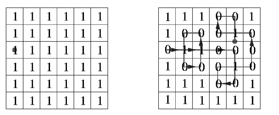
FIG. 1.: Illustration of the data corruption process for $d=2$. The initial uncorrupted state is shown on the left, with the BA represented by the filled circle. On the right we show a typical walk of $\sim 20$ steps. The BA flips a spin with each visit, so those spins visited an even number of times are restored to their original value.

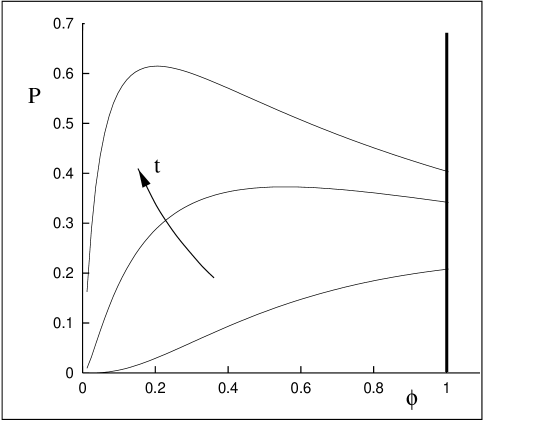
FIG. 2.: ${\cal P}(\phi,x,t)$ versus $\phi$, as given in Eq.(65), with $x=1,{\tilde{\lambda}}=\sqrt{2}$, for three different times, $t=0.5,\ 1.0,\ 1.5$. The thick vertical line represents the $\delta$-function at $\phi=1$.

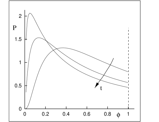
FIG. 3.: ${\cal P}(\phi,0,t)$ versus $\phi$, as given in Eq.(66), for three different times.

FIG. 4.: Log-log plot of $m_{0}(t)$ (diamonds) and $\sum_{R}\Theta(R,t,R)$ (plusses) versus time from $d=1$ numerical simulation. The solid line is the asymptotic theoretical prediction (31).

FIG. 5.: Log-log plot of $m_{x}(t)-m_{0}(t)$ versus $x/\sqrt{t}$ for a time of $10^{3}$ in $d=1$. The solid line is the theoretical prediction (32).

FIG. 6.: Log-log plot of $1-m_{0}(t)$ versus $x/\sqrt{t}$ for times $10^{3}$ and $10^{4}$ in $d=1$. Also shown is the theoretical prediction (33) for the intermediate regime.

FIG. 7.: Log-log plot of the time derivative of the total number of minus spins (diamonds) and of $m_{0}(t)$ (plusses) versus time in $d=1$. The solid line is the theoretical prediction (31).

FIG. 8.: The ratio $C_{x}(t)/m_{0}(t)$ plotted against $x/\sqrt{t}$ for times of $100$ (plusses) and $500$ (diamonds) in $d=1$. The solid line is the theoretical prediction (53).

FIG. 9.: Linear-log plot of $1/m_{\bf 0}(t)$ versus time for $d=2$. The solid line is the theoretical prediction (88).

FIG. 10.: Probability distribution of patch (21 spins) magnetization for times of $10^{2}$, $10^{3}$, and $10^{4}$ in $d=1$. Note the robust tail for values of patch magnetization near unity.

REFERENCES

- [1] R. Brown, Philos. Mag. Ann. of Philos. New Ser. 4, 161 (1823).
- [2] A. Einstein, Ann. der Physik 17, 549 (1905).
- [3] B. D. Hughes, Random Walks and Random Environments, (Clarendon Press, Oxford, 1995); C. Itzykson and J.-M. Drouffe, Statistical Field Theory, (Cambridge University Press, 1989).
- [4] J-P. Bouchaud and A. Georges, Phys. Rep., 195, 127 (1990).
- [5] J. Bernasconi, H. Beyeler, S. Strässler and S. Alexander, Phys. Rev. Lett., 42, 819 (1979).
- [6] J. R. Manning, Diffusion Kinetics for Atoms in Crystals, (Van Nostrand, Princeton N.J., 1968).
- [7] M. J. A. M. Brummelhuis and H. J. Hilhorst, J. Stat. Phys., 53, 249 (1988).
- [8] T. J. Newman, preprint cond-mat/9806291.
- [9] Z. Toroczkai, G. Korniss, B. Schmittmann and R. K. P. Zia, Europhys Lett, 40, 281 (1997).
- [10] W. Th. F. den Hollander and P. W. Kasteleyn, Physica, 117A, 179 (1983); J. Stat. Phys., 39, 15 (1985).
- [11] S. Middelhoek, P. K. George and P. Dekker, Physics of Computer Memory Devices (Academic Press, London, 1976).
- [12] A. K. Sharma, Semiconductor Memories (IEEE Press, Piscataway NJ, 1996).
- [13] For more diverse examples see I. S. Herschberg and R. Paans, Informatie, 28, 10 (1986); F. B. Cohen, in Information Security - the Next Decade, eds. J. H. P. Eloff and S. H. von Solms (Chapman and Hall, London, 1995).
- [14] C. W. Gardiner, Handbook of Stochastic Processes, 2nd ed. (Springer-Verlag, Berlin, 1985).
- [15] L. D. Landau and E. M. Lifschitz, Quantum Mechanics (Pergamon Press, London 1958).
- [16] Theory and Applications of Cellular Automata, ed. S. Wolfram, (World Scientific, Singapore, 1987); F. Bagnoli in Dynamical Modelling in Biotechnologies, eds. F. Bagnoli, P. Lio and S. Ruffo, (World Scientific, Singapore, 1998)
- [17] H. E. Stanley, Introduction to Phase Transitions and Critical Phenomena, (Oxford University Press, 1971).
- [18] R. P. Feynman and A. Hibbs, Quantum Mechanics and Path Integrals (McGraw-Hill, New York, 1965); L. S. Schulman, Techniques and Applications of Path Integration (Wiley, New York, 1981).
- [19] Handbook of Mathematical Functions 10th Edition, M. Abramowitz and I. A. Stegun Eds. (Dover, NY, 1972).
- [20] H. Jeffreys and B. Jeffreys, Methods of Mathematical Physics 3rd Edition (Cambridge University Press, Cambridge, 1980).
- [21] Point Defects in Solids, eds. J. H. Crawford and L. M. Slifkin (Plenum Press, New York, 1976); F. Agullo-Lopez, C. R. A. Catlow and P. D. Townsend, Point Defects in Materials (Academic Press, London, 1988).