Director Field Configurations around a Spherical Particle in a Nematic Liquid Crystal

Abstract

We study the director field around a spherical particle immersed in a uniformly aligned nematic liquid crystal and assume that the molecules prefer a homeotropic orientation at the surface of the particle. Three structures are possible: a dipole, a Saturn-ring, and a surface-ring configuration, which we investigate by numerically minimizing the Frank free energy supplemented by a magnetic-field and a surface term. In the dipole configuration, which is the absolutely stable structure for micron-size particles and sufficiently strong surface anchoring, a twist transition is found and analyzed. We show that a transition from the dipole to the Saturn ring configuration is induced by either decreasing the particle size or by applying a magnetic field. The effect of metastability and the occurence of hysteresis in connection with a magnetic field are discussed. The surface-ring configuration appears when the surface-anchoring strength $W$ is reduced. It is also favored by a large saddle-splay constant $K_{24}$. A comparison with recent experiments [10, 13] gives a lower bound for W, i.e., $W>0.6\,\text{erg}/\text{cm}^{2}$ for the interface of water and pentylcyanobiphenyl (5CB) in the presence of the surfactant sodium dodecyl sulfate.

]

I Introduction

Dispersions of particles in a host fluid are part of our everyday life and an important matter of state. Since they appear in food (e.g. milk), drugs, paints, and ink, they are of considerable technological importance. In colloidal suspensions the particles are solid, whereas emulsions are dispersions of liquid droplets coated with a surfactant. There exists a whole zoo of interactions between the particles whose delicate balance determines the stability of a dispersion. Besides the conventional van-der-Waals, screened Coulombic, and steric interactions [1], fluctuation-induced Casimir forces [2, 3] and depletion forces [1, 4, 5, 6] have attracted a lot of interest.

When the particles are dispersed in a nematic liquid crystal, i.e., an anisotropic fluid, where elongated organic molecules are aligned on average along a common direction called director, additional long-range forces due to elastic deformations of the director field are induced. These forces are of dipolar or quadrupolar type depending on the symmetry of the director configuration around the particle [7, 8, 9, 10, 11], and they were confirmed by recent experiments in inverted nematic emulsions [10, 12, 13]. On the other hand topological point defects in the orientational order of the molecules give rise to a short-range repulsion [10, 13]. Related early work deals with forces between walls mediated by an enclosed nematic liquid crystal [14, 15]. Surface-induced nematic order in the isotropic phase close to the isotropic-nematic phase transition leads to a short-range interaction as reported in most recent experimental and theoretical work [16, 17, 18, 19]. Even Casimir forces arising from fluctuations in the liquid crystalline order parameter have been calculated [20, 21, 22].

Before treating the interaction between particles it is necessary to understand how one single particle behaves in a nematic environment. This article deals with the possible director configurations around a spherical particle, which is placed into a uniformly aligned nematic liquid crystal, and which prefers a homeotropic, i.e., perpendicular anchoring of the molecules at its surface. This is already a complicated problem. Since it cannot be solved analytically without employing an ansatz function for the director configuration and further approximations, we will handle it by numerical methods.

Poulin et al. showed experimentally that in inverted nematic emulsions, where surfactant-coated water droplets are dispersed in a nematic liquid crystal, a director field configuration of dipolar symmetry occurs (see Fig. 1) [10, 13]. The water droplet and its companion hyperbolic point defect form a tightly bound object which we call dipole for short. A similar observation at a nematic-isotropic interface was made by R. B. Meyer much earlier [23]. Both the droplet and the defect carry a topological charge $+1$, which “add up” to the total charge 0 of the dipole [24]. Theoretically it was described with the help of ansatz functions that were motivated by an electrostatic analog [10, 11]. Terentjev et al. introduced the Saturn-ring configuration with quadrupolar symmetry where a $-1/2$ disclination ring surrounds the sphere at the equator (see Fig. 1). It was investigated by both analytic and numerical methods [25, 26]. By shrinking the disclination ring to the topologically equivalent hyperbolic point defect, the Saturn ring can be continuously transformed into the dipole configuration [11]. With the help of an ansatz function that describes such a transformation it was conjectured that for sufficently small particles the Saturn ring should be more stable than the dipole [11]. For a finite anchoring strength of the molecules at the surface a third structure occurs, which we also illustrate in Fig. 1. We call it the surface-ring configuration. Depending on the anchoring strength $W$ there exists either a $-1/2$ disclination ring sitting directly at the surface, or, for smaller $W$ [26], the director field is smooth everywhere, and a ring of tangentially oriented molecules is located at the equator of the sphere. By means of a Monte-Carlo simulation Ruhwandl and Terentjev showed that for sufficently small anchoring strength $W$ the surface ring is the preferred configuration [27].

In this article we give a full account of the three director configurations in Fig. 1 by numerically minimizing the Frank free energy supplemented by a magnetic-field and a surface term [28]. We go beyond the one-constant approximation, generally used in the work cited above, and include the saddle-splay term of the Frank free energy. Furthermore, the results of the analytic approach based on the use of ansatz functions are checked. In particular, we investigate the dipole configuration, which undergoes a twist transition. Then, we show in detail that the transition from the dipole to the Saturn ring configuration can be either achieved by decreasing the particle size or by applying a magnetic field. The role of metastability is discussed. Finally, the surface ring is considered, and the special role of the saddle-splay free energy for its occurence is pointed out. Lower bounds for the surface-anchoring strength $W$ are given. All these results are presented in Sec. III. In Sec. II we define the geometry of our problem, write down the reduced free energy, and explain the numerical method to minimize it.

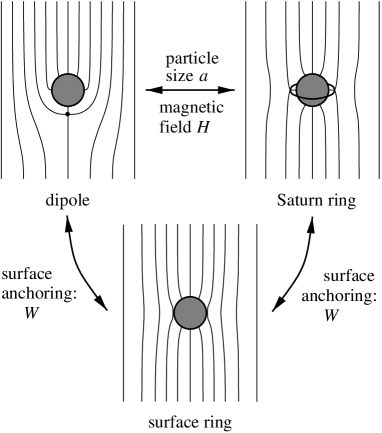
FIG. 1.: A spherical particle with a preferred homeotropic anchoring at its surface that is placed into a uniformly aligned nematic liquid crystal exhibits three possible structures: the dipole configuration where the particle is accompanied by a hyperbolic hedgehog, the Saturn-ring configuration where the particle is surrounded by a $-1/2$ disclination ring at the equator, and the surface-ring configuration.

FIG. 2.: Illustration of the modified spherical coordinates ($\rho=1/r^{2},\theta$). At each point the local coordinate basis $({\bf e}_{r},{\bf e}_{\theta},{\bf e}_{\phi})$ of the standard spherical coordinate system is attached. The integration area is given by $0\leq\rho\leq 1$.

II Geometry, Free Energy, and Numerical Method

The director field around a spherical particle follows from the minimization of the Frank free energy supplemented by a magnetic-field and a surface term. In this section we describe our coordinate system, review the free energy, and give some numerical details.

A Geometry

The region outside the spherical particle with radius $a$ is infinitely extended. We use a modified spherical coordinate system with a radial coordinate $\rho=1/r^{2}$ where $r$ is the distance of a space point from the center of the particle measured in units of $a$. The exponent 2 is motivated by the far-field of the dipol configuration [10, 11]. Such a transformation has two advantages. The exterior of the particle is mapped into a finite region, i.e., the interior of the unit sphere ($\rho\leq 1$). Furthermore, equally spaced grid points along the coordinate $\rho$ result in a mesh size in real space which is small close to the surface of the particle. In this area the director field is strongly varying, and hence a good resolution for the numerical calculation is needed. On the other hand, the mesh size is large far away from the sphere where the director field is nearly homogeneous. Since our system is axially symmetric, the director field only depends on $\rho$ and the polar angle $\theta$ as illustrated in Fig. 2. The symmetry axis corresponds to the $z$ axis. At each point $(\rho,\theta)$ we attach the local coordinate basis $({\bf e}_{r},{\bf e}_{\theta},{\bf e}_{\phi})$ of the standard spherical coordinate system and express the director in this basis:

$${\bf n}(\rho,\theta)=n_{r}(\rho,\theta){\bf e}_{r}+n_{\theta}(\rho,\theta){\bf e}_{\theta}+n_{\phi}(\rho,\theta){\bf e}_{\phi}\enspace.$$ (1)

Since the director is a unit vector, we write

$$n_{r}=\cos\Theta\enspace,\enspace n_{\theta}=\sin\Theta\cos\Phi\enspace,\enspace n_{\phi}=\sin\Theta\sin\Phi\enspace,$$ (2)

where $\Theta(\rho,\theta)$ and $\Phi(\rho,\theta)$ denote, respectively, the tilt and the twist angle. At the surface of the particle we allow the director to rotate away from the preferred radial direction by introducing a surface free energy (see next subsection). At infinity, i.e., at $\rho=0$ ${\bf n}$ always points along the $z$ axis. For completeness we note that the differentials $dr$ and $d\rho$ are connected via

$$dr=-d\rho/(2\rho^{3/2})\enspace.$$ (3)

B Free energy

The free energy which we will minimize consists of bulk and surface terms:

$$F_{\bf n}=\int d^{3}x(f_{el}+f_{24}+f_{H})+\int dSf_{S}\enspace$$ (4)

with the free energy densities:

$$f_{el} = \frac{1}{2}\{K_{1}(\mathchoice{{\hbox{\boldmath$\displaystyle\nabla$}}}{{\hbox{\boldmath$\textstyle\nabla$}}}{{\hbox{\boldmath$\scriptstyle\nabla$}}}{{\hbox{\boldmath$\scriptscriptstyle\nabla$}}}\cdot{\bf n})^{2}+K_{2}({\bf n}\cdot\mathchoice{{\hbox{\boldmath$\displaystyle\nabla$}}}{{\hbox{\boldmath$\textstyle\nabla$}}}{{\hbox{\boldmath$\scriptstyle\nabla$}}}{{\hbox{\boldmath$\scriptscriptstyle\nabla$}}}\times{\bf n})^{2}$$ (7)

$$+K_{3}[{\bf n}\times(\mathchoice{{\hbox{\boldmath$\displaystyle\nabla$}}}{{\hbox{\boldmath$\textstyle\nabla$}}}{{\hbox{\boldmath$\scriptstyle\nabla$}}}{{\hbox{\boldmath$\scriptscriptstyle\nabla$}}}\times{\bf n})]^{2}\}$$

$$f_{24}=-\frac{1}{2}K_{24}\mathchoice{{\hbox{\boldmath$\displaystyle\nabla$}}}{{\hbox{\boldmath$\textstyle\nabla$}}}{{\hbox{\boldmath$\scriptstyle\nabla$}}}{{\hbox{\boldmath$\scriptscriptstyle\nabla$}}}\cdot[{\bf n}(\mathchoice{{\hbox{\boldmath$\displaystyle\nabla$}}}{{\hbox{\boldmath$\textstyle\nabla$}}}{{\hbox{\boldmath$\scriptstyle\nabla$}}}{{\hbox{\boldmath$\scriptscriptstyle\nabla$}}}\cdot{\bf n})+{\bf n}\times(\mathchoice{{\hbox{\boldmath$\displaystyle\nabla$}}}{{\hbox{\boldmath$\textstyle\nabla$}}}{{\hbox{\boldmath$\scriptstyle\nabla$}}}{{\hbox{\boldmath$\scriptscriptstyle\nabla$}}}\times{\bf n})]$$ (8)

$$f_{H}=-\frac{1}{2}\Delta\chi[({\bf n}\cdot{\bf H})^{2}-H^{2}]$$ (9)

$$f_{S}=\frac{1}{2}W[1-({\bf n}\cdot\hat{\mathchoice{{\hbox{\boldmath$\displaystyle\nu$}}}{{\hbox{\boldmath$\textstyle\nu$}}}{{\hbox{\boldmath$\scriptstyle\nu$}}}{{\hbox{\boldmath$\scriptscriptstyle\nu$}}}})^{2}]\enspace.$$ (10)

The Oseen-Zöcher-Frank free energy density $f_{el}+f_{24}$ describes elastic distortions of the director field ${\bf n}({\bf r})$, where $K_{1}$, $K_{2}$, $K_{3}$, and $K_{24}$ denote, respectively, the splay, twist, bend, and saddle-splay elastic constants. The saddle-splay term is a pure divergence; it, therefore, can be transformed into integrals over all surfaces of the system. A Cauchy relation for $K_{24}$ follows from the Maier-Saupe molecular approach [29]:

$$K_{24}=(K_{11}+K_{22})/2\enspace.$$ (11)

(There is also the possibility of another surface term with a free energy density $K_{13}\mathchoice{{\hbox{\boldmath$\displaystyle\nabla$}}}{{\hbox{\boldmath$\textstyle\nabla$}}}{{\hbox{\boldmath$\scriptstyle\nabla$}}}{{\hbox{\boldmath$\scriptscriptstyle\nabla$}}}\cdot({\bf n}\mathchoice{{\hbox{\boldmath$\displaystyle\nabla$}}}{{\hbox{\boldmath$\textstyle\nabla$}}}{{\hbox{\boldmath$\scriptstyle\nabla$}}}{{\hbox{\boldmath$\scriptscriptstyle\nabla$}}}\cdot{\bf n})$, which we will not consider in this paper.) Eq. (9) couples the director to an external magnetic field ${\bf H}$, where $\Delta\chi=\chi_{\|}-\chi_{\perp}$ stands for the magnetic anisotropy. The symbols $\chi_{\|}$ and $\chi_{\perp}$ denote the magnetic susceptibilities for a magnetic field applied, respectively, parallel or perpendicular to the director. In this paper we consider a positive $\Delta\chi$ that favors an alignment of the director ${\bf n}$ parallel to ${\bf H}$. Since we calculate the magnetic free energy of the infinitely extended region around the sphere, we use the magnetic free energy of a completely aligned director field as a reference point to avoid infinities. As a result the term $-\Delta\chi H^{2}/2$ in Eq. (9) occurs. Finally, we employ the surface free energy of Rapini-Papoular to take into account the interaction of the director with the boundaries. In Eq. (10) the unit vector $\hat{\mathchoice{{\hbox{\boldmath$\displaystyle\nu$}}}{{\hbox{\boldmath$\textstyle\nu$}}}{{\hbox{\boldmath$\scriptstyle\nu$}}}{{\hbox{\boldmath$\scriptscriptstyle\nu$}}}}$ denotes some preferred orientation of the director at the surface, and $W$ is the coupling constant. It varies in the range $10^{-4}-1$ erg/cm² as reviewed by Blinov et al. [30]. However, the authors do not specify $W$ for the interface of water and the liquid-crystalline phase of 5CB in the presence of the surfactant sodium dodecyl sulfate, which was used in the experiment by Poulin et al. [10, 13]. In subsection III C we will give a lower bound for $W$ for such an interface.

For the numerical minimization a reduced form of the free energy of Eq. (4) is used. We introduce the energy unit $\pi K_{3}a$ and refer all lengths to the radius $a$ of the spherical particle. Furthermore, we employ the modified spherical coordinates ($\rho,\theta$), take into account the axial symmetry of our system, and, finally, arrive at the reduced free energy

$$\overline{F}_{\bf n} = F_{\bf n}/(\pi K_{3}a)$$ (12)

$$= \int_{\rho\leq 1}d\theta d\rho\frac{\sin\theta}{\rho^{5/2}}(\overline{f}_{el}+\overline{f}_{24}+\overline{f}_{H})+\int_{\rho=1}d\theta\sin\theta\overline{f}_{S}\enspace,$$ (13)

where

$$\overline{f}_{el} = \frac{1}{2}\{\overline{K}_{1}(\mathchoice{{\hbox{\boldmath$\displaystyle\nabla$}}}{{\hbox{\boldmath$\textstyle\nabla$}}}{{\hbox{\boldmath$\scriptstyle\nabla$}}}{{\hbox{\boldmath$\scriptscriptstyle\nabla$}}}\cdot{\bf n})^{2}+\overline{K}_{2}({\bf n}\cdot\mathchoice{{\hbox{\boldmath$\displaystyle\nabla$}}}{{\hbox{\boldmath$\textstyle\nabla$}}}{{\hbox{\boldmath$\scriptstyle\nabla$}}}{{\hbox{\boldmath$\scriptscriptstyle\nabla$}}}\times{\bf n})^{2}$$ (16)

$$+[{\bf n}\times(\mathchoice{{\hbox{\boldmath$\displaystyle\nabla$}}}{{\hbox{\boldmath$\textstyle\nabla$}}}{{\hbox{\boldmath$\scriptstyle\nabla$}}}{{\hbox{\boldmath$\scriptscriptstyle\nabla$}}}\times{\bf n})]^{2}\}$$

$$\overline{f}_{24}=-\frac{1}{2}\overline{K}_{24}\mathchoice{{\hbox{\boldmath$\displaystyle\nabla$}}}{{\hbox{\boldmath$\textstyle\nabla$}}}{{\hbox{\boldmath$\scriptstyle\nabla$}}}{{\hbox{\boldmath$\scriptscriptstyle\nabla$}}}\cdot[{\bf n}(\mathchoice{{\hbox{\boldmath$\displaystyle\nabla$}}}{{\hbox{\boldmath$\textstyle\nabla$}}}{{\hbox{\boldmath$\scriptstyle\nabla$}}}{{\hbox{\boldmath$\scriptscriptstyle\nabla$}}}\cdot{\bf n})+{\bf n}\times(\mathchoice{{\hbox{\boldmath$\displaystyle\nabla$}}}{{\hbox{\boldmath$\textstyle\nabla$}}}{{\hbox{\boldmath$\scriptstyle\nabla$}}}{{\hbox{\boldmath$\scriptscriptstyle\nabla$}}}\times{\bf n})]$$ (17)

$$\overline{f}_{H}=-\frac{1}{2}\xi_{H}^{-2}[(n_{r}\cos\theta-n_{\theta}\sin\theta)^{2}-1]$$ (18)

$$\overline{f}_{S}=\xi_{S}^{-1}(1-n_{r}^{2})\enspace.$$ (19)

In Eqs. (16) and (17) the coefficients $\overline{K}_{1}=K_{1}/K_{3}$, $\overline{K}_{2}=K_{2}/K_{3}$, and $\overline{K}_{24}=K_{24}/K_{3}$ denote, respectively, the reduced splay, twist, and saddle-splay elastic constants. The single contributions to the Frank free energy density in our modified spherical coordinates are rather lengthy, and we refer the reader to Appendix A for the detailed form. We always apply the magnetic field ${\bf H}$ along the symmetry axis of our system, which coincides with the $z$ axis (see Fig. 2). Inserting ${\bf H}=H{\bf e}_{z}$ with ${\bf e}_{z}=\cos\theta{\bf e}_{r}-\sin\theta{\bf e}_{\theta}$ into Eq. (9) we obtain the magnetic free energy density of Eq. (18). The strength of the field is given via the reduced magnetic coherence length:

$$\xi_{H}=\sqrt{K_{3}/(\Delta\chi H^{2})}/a\enspace.$$ (20)

It indicates the distance in the bulk which is needed to orient the director along the applied field when, e.g., through boundary conditions a different preferred orientation of the molecules exists [28]. The length tends to infinity for $H\rightarrow 0$. The surface term of Eq. (19) follows from Eq. (10) by choosing $\hat{\mathchoice{{\hbox{\boldmath$\displaystyle\nu$}}}{{\hbox{\boldmath$\textstyle\nu$}}}{{\hbox{\boldmath$\scriptstyle\nu$}}}{{\hbox{\boldmath$\scriptscriptstyle\nu$}}}}={\bf e}_{r}$, i.e., a preferred radial anchoring of the molecules at the surface of the suspended particle. The reduced extrapolation length [28]

$$\xi_{S}=K_{3}/(Wa)$$ (21)

signifies the strength of the anchoring. It compares the Frank free energy of the bulk, which is proportional to $K_{3}a$, to the surface energy, which scales with $Wa^{2}$. At strong anchoring, i.e., for $\xi_{S}\ll 1$ the energy to rotate the director away from its preferred direction $\hat{\mathchoice{{\hbox{\boldmath$\displaystyle\nu$}}}{{\hbox{\boldmath$\textstyle\nu$}}}{{\hbox{\boldmath$\scriptstyle\nu$}}}{{\hbox{\boldmath$\scriptscriptstyle\nu$}}}}$ at the whole surface would be much larger than the bulk energy. Therefore, it is preferable for the system when the director points along $\hat{\mathchoice{{\hbox{\boldmath$\displaystyle\nu$}}}{{\hbox{\boldmath$\textstyle\nu$}}}{{\hbox{\boldmath$\scriptstyle\nu$}}}{{\hbox{\boldmath$\scriptscriptstyle\nu$}}}}$. However, ${\bf n}$ can deviate from $\hat{\mathchoice{{\hbox{\boldmath$\displaystyle\nu$}}}{{\hbox{\boldmath$\textstyle\nu$}}}{{\hbox{\boldmath$\scriptstyle\nu$}}}{{\hbox{\boldmath$\scriptscriptstyle\nu$}}}}$ in the area $\xi_{S}a^{2}$. This will explain the result in subsection III C where we show that the surface ring already appears at strong surface coupling. Rigid anchoring is realized for $\xi_{S}\rightarrow 0$, and $\xi_{S}\gg 1$ means weak anchoring, where the influence of the surface is minor.

To calculate the free energy $\overline{F}_{\bf n}$ numerically we transform the saddle-splay term into a surface integral:

$$\overline{F}_{24}=\overline{K}_{24}\int_{\rho=1}d\theta\sin\theta{\bf e}_{r}\cdot[{\bf n}(\mathchoice{{\hbox{\boldmath$\displaystyle\nabla$}}}{{\hbox{\boldmath$\textstyle\nabla$}}}{{\hbox{\boldmath$\scriptstyle\nabla$}}}{{\hbox{\boldmath$\scriptscriptstyle\nabla$}}}\cdot{\bf n})+{\bf n}\times(\mathchoice{{\hbox{\boldmath$\displaystyle\nabla$}}}{{\hbox{\boldmath$\textstyle\nabla$}}}{{\hbox{\boldmath$\scriptstyle\nabla$}}}{{\hbox{\boldmath$\scriptscriptstyle\nabla$}}}\times{\bf n})]\enspace.$$ (22)

The detailed form follows from Appendix A. In performing Gauss’ theorem we only include the surface of the sphere. There is also a contribution from the surface of the core of a possible disclination ring. However, since we can only describe the energy of the core in an approximate way (see next paragraph), we will skip this term. For rigid homeotropic anchoring ($n_{r}=1$, $n_{\theta}=n_{\phi}=0$) the free energy of the saddle-splay term is

$$\overline{F}_{24}=4\overline{K}_{24}\enspace.$$ (23)

To arrive at Eq. (23) we used $\partial n_{r}/\partial\rho=0$, which is valid because of the normalization of the director.

The free energy of a $\pm\frac{1}{2}$ disclination ring is taken into account by the line energy $F_{d}$ of a $\pm\frac{1}{2}$ disclination. In the one-constant approximation ($K_{1}=K_{2}=K_{3}=K$) and in reduced units it reads [31]

$$\overline{F}_{d}=F_{d}/K=\frac{\pi}{4}\left(\frac{1}{2}+\ln\frac{R}{r_{c}}\right)\enspace.$$ (24)

The first term denotes the line energy of the core with a core radius $r_{c}$ which in absolute lengths is of the order of $10\,\text{nm}$. The second term stands for the elastic energy of the disclination line where $R$ is its radial extent [see Fig. 3b)]. In the general case ($K_{1}\neq K_{2}\neq K_{3}$) an analytic expression for the elastic energy does not exist. We only use a rough approximation for the core energy $F_{c}$ by averaging over the Frank constants:

$$\overline{F}_{c}=F_{c}/K_{3}=\frac{\pi}{8}(\overline{K}_{1}+\overline{K}_{2}+1)/3\enspace.$$ (25)

A more quantitative description of the free energy of a disclination has to start from the Landau-Ginzburg-de Gennes free energy with the full alignment tensor ${\bf Q}$ [32, 33].

We finish this subsection with an important remark about length scales. In the free energy of Eq. (12) all lengths are given relative to the particle radius $a$, which appears in the absolute energy unit $\pi K_{3}a$ only. This would suggest that the director configuration does not depend on the particle size. However, with the core radius $r_{c}$ a second length scale is introduced, which in absolute lengths is always of the order of $10\,\text{nm}$ [31]. On the other hand, in the next subsection we explain that $r_{c}$ in units of $a$ is a parameter of our numerical method whose lower bound is determined by the mesh size of the grid. In the discussions of Sec. III we want to make a connection to experiments. Therefore, we do not give this dimensionless $r_{c}$, but use an absolute core size of $10\,\text{nm}$ to calculate the corresponding particle radius $a$:

$$a=10\,\text{nm}/r_{c}\enspace.$$ (26)

In subsection III B 1 we will study how the configuration around a spherical particle depends on $a$.

C Minimization and numerical details

The fields of the tilt [$\Theta(\rho,\theta)$] and the twist [$\Phi(\rho,\theta)$] angle follow from a minimization of the reduced free energy $\overline{F}_{\bf n}[\Theta,\Phi]$ of Eq. (12). The corresponding Euler-Lagrange equations are equivalent to the functional derivatives of $\overline{F}_{\bf n}[\Theta,\Phi]$:

$$\frac{\delta\overline{F}_{\bf n}}{\delta\Theta} = \frac{\delta\overline{F}_{\bf n}}{\delta n_{i}}\frac{\partial n_{i}}{\partial\Theta}=0$$ (27)

$$\frac{\delta\overline{F}_{\bf n}}{\delta\Phi} = \frac{\delta\overline{F}_{\bf n}}{\delta n_{i}}\frac{\partial n_{i}}{\partial\Phi}=0\enspace,$$ (28)

where $i$ stands for $r$, $\theta$, and $\phi$ and Einstein’s summation convention over repeated indices is used. We have employed a chain rule to arrive at the Euler-Lagrange equations for $\Theta(\rho,\theta)$ and $\Phi(\rho,\theta)$, which is generally valid for functional derivatives as shown in Appendix B. Performing the variation of the free energy $\overline{F}_{\bf n}$ we arrive at the Euler-Lagrange equations in the bulk,

$$\left[\left(\frac{\partial}{\partial n_{i}}-\frac{\partial}{\partial x_{j}}\frac{\partial}{\partial n_{i,j}}\right)\frac{\sin\theta}{\rho^{5/2}}(\overline{f}_{el}+\overline{f}_{H})\right]\frac{\partial n_{i}}{\partial\Theta} = 0$$ (29)

$$\left[\left(\frac{\partial}{\partial n_{i}}-\frac{\partial}{\partial x_{j}}\frac{\partial}{\partial n_{i,j}}\right)\frac{\sin\theta}{\rho^{5/2}}(\overline{f}_{el}+\overline{f}_{H})\right]\frac{\partial n_{i}}{\partial\Phi} = 0\enspace,$$ (30)

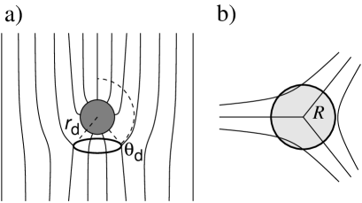
FIG. 3.: a) Coordinates ($r_{d},\theta_{d}$) for a -1/2 disclination ring with a general position around the spherical particle; b) Cross section of the $-1/2$ disclination ring with a radial extension $R$.

and at the surface,

$$\left(\frac{\partial\overline{f}_{S}}{\partial n_{i}}+\frac{\partial}{\partial n_{i,\rho}}(\overline{f}_{el}+\overline{f}_{24})\right)\frac{\partial n_{i}}{\partial\Theta} = 0$$ (31)

$$\left(\frac{\partial\overline{f}_{S}}{\partial n_{i}}+\frac{\partial}{\partial n_{i,\rho}}(\overline{f}_{el}+\overline{f}_{24})\right)\frac{\partial n_{i}}{\partial\Phi} = 0\enspace,$$ (32)

where $n_{i,j}$ stands for $\partial n_{i}/\partial x_{j}$. The Euler-Lagrange equations are calculated with the help of the algebraic program Maple and are then imported into a Fortran program where they are usually solved on a rectangular $33\times 129$ grid in the $(\rho,\theta)$ space. In Eq. (33) of ref. [11] an analytical form of the director configuration of a $-\frac{1}{2}$ disclination ring around a spherical particle is given. The position of this ring is determined by the radial ($r_{d}$) and the angular ($\theta_{d}$) coordinates [see Fig. 3a)]. We take this director configuration and let it relax via the standard Newton-Gauss-Seidel method [34]. In the dipole configuration ($\theta_{d}=0,\pi$) the hyperbolic point defect moves along the $z$ axis in its local minimum when the numerical relaxation is performed. However, a disclination ring ($\theta_{d}\neq 0,\pi$) basically stays at the positon where we place it. We use this fact to investigate the free energy as a function of $r_{d}$ and $\theta_{d}$ which gives an instructive insight into potential barriers for a transition between the dipole and the Saturn-ring configuration.

The free energy $\overline{F}_{\bf n}$ of the director field follows from a numerical integration. This procedure assigns some energy to the disclination ring which certainly is not correct. To obtain a more accurate value for the total free energy $\overline{F}$ we use the formula

$$\overline{F}=\overline{F}_{\bf n}-\left.\overline{F}_{\bf n}\right|_{\text{torus}}+\overline{F}_{c/d}\times 2\pi r_{d}\sin\theta_{d}\enspace.$$ (33)

The quantity $\left.\overline{F}_{\bf n}\right|_{\text{torus}}$ denotes the numerically calculated free energy of a toroidal region of cross section $\pi R^{2}$ around the disclination ring [see Fig. 3b)]. Its volume is $\pi R^{2}\times 2\pi r_{d}\sin\theta_{d}$, where the coordinates $(r_{d},\theta_{d})$ of the ring are determined by searching for the maximum of the local free energy density $\overline{f}_{el}$. The value $\left.\overline{F}_{\bf n}\right|_{\text{torus}}$ is replaced by the last term on the right-hand side of Eq. (33), which provides the correct free energy according to Eqs. (24) or (25). To find out how large the cross section $\pi R^{2}$ of the cut torus has to be, we employed the last formula and the line energy of Eq. (24) for constant $r_{c}$ and varying $R$. To be consistent, $\overline{F}$ should not depend on $R$. Within an error of less than 1 % this is the case if $\pi R^{2}$ is equal or larger than $3\Delta\rho\Delta\theta/2$ where $\Delta\rho$ and $\Delta\theta$ are the lattice constants of our grid. To study the transition between the dipole and the Saturn ring as a function of the particle size we choose $\pi R^{2}=25\Delta\rho\Delta\theta/2$, employ Eq. (24) for different $r_{c}$, and calculate $a$ from Eq. (26). In all other cases we set $R=r_{c}$, determine $r_{c}$ from $\pi r^{2}_{c}=3\Delta\rho\Delta\theta/2$, and use the core energy of Eq. (25).

The radial extension of the core of a point defect is also of the order of 10 nm [35], and its free energy is approximated by $K_{3}\times 10\,\mathrm{nm}$. As we show in the following section the free energy of the dipole amounts to around $10\pi K_{3}a$. Since we consider particle radii larger than $100\,\mathrm{nm}$, the contribution from the energy of the point defect is always smaller than 1 %. This is beyond our numerical accuracy, and therefore no energetical correction for the point defect was included.

The discussion in the following section always uses the one-constant approximation or the nematic liquid crystal pentylcyanobiphenyl (5CB) with the bend elastic constant $K_{3}=0.53\times 10^{-6}\,\mathrm{dyn}$ and the reduced splay and twist elastic constants $\overline{K}_{1}=0.79$ and $\overline{K}_{2}=0.43$, respectively.

III Results and Discussion

In this section we present the results of our numerical investigation. We first address a twist transition in the dipole configuration. Then we discuss a transition from the dipole to the Saturn ring which is induced either by decreasing the particle size or by applying a magnetic field. Finally, we illustrate that the surface-ring configuration appears when the surface-anchoring strength is lowered.

A Twist transition of the dipole configuration

In Fig. 4 we plot the director field of the dipole configuration for the one-constant approximation. A magnetic field is not applied and the directors are rigidly anchored at the surface. The dot indicates the location of the hyperbolic hedgehog. For its distance $r_{d}$ from the center of the sphere we find $r_{d}=1.26\pm 0.02$, where the mesh size of the grid determines the uncertainty in $r_{d}$. Our result is in excellent agreement with Ref. [11]. In this article the dipole was described via an ansatz function. However, Ruhwandl and Terentjev using a Monte-Carlo minimization report a somewhat smaller value for $r_{d}$ [9].

Fig. 5 presents the distance $r_{d}$ as a function of the reduced splay ($\overline{K}_{1}$) and twist ($\overline{K}_{1}$) constants. In front

FIG. 4.: The numerically determined director field of the dipole configuration for the one-constant approximation, zero magnetic field, and rigid surface anchoring. The location of the hyperbolic hedgehog is indicated by a dot. The directors lie in the drawing plane.

of the thick line $r_{d}$ is basically constant. Beyond the line $r_{d}$ starts to grow which indicates a structural change in the director field illustrated in the nail picture of Fig. 6. Around the hyperbolic hedgehog the directors develop a non-zero azimuthal component $n_{\phi}$ introducing a twist into the dipole. It should be visible under a polarizing microscope when the dipole is viewed along its symmetry axis.

In Fig. 7 we draw a phase diagram for the twist transition. As expected, it occurs when $\overline{K}_{1}$ increases or when $\overline{K}_{2}$ decreases, i.e., when a twist deformation costs less energy than a splay distortion. The open circles are nu-

FIG. 5.: The distance $r_{d}$ of the hyperbolic hedgehog from the center of the sphere as a function of the reduced splay ($\overline{K}_{1}$) and twist ($\overline{K}_{2}$) constants.

FIG. 6.: Nail picture of a close-up of the twisted dipole configuration. Around the hyperbolic hedgehog the directors are tilted out of the drawing plane. The length of the nail is proportional to the projection of the director on the drawing plane. The head of the nail is below the plane.

merical results for the transition line which can be well fitted by the straight line $\overline{K}_{2}\approx\overline{K}_{1}-0.04$. Interestingly, the small offset $0.04$ means that $K_{3}$ does not play an important role. Typical calamatic liquid crystals like MBBA, 5CB, and PAA should show the twisted dipole configuration.

Since the twist transition breaks the mirror symmetry of the dipole, which then becomes a chiral object, we describe it by a Landau expansion of the free energy:

$$F=F_{0}+a(\overline{K}_{1},\overline{K}_{2})[n_{\phi}^{\text{max}}]^{2}+c[n_{\phi}^{\text{max}}]^{4}\enspace.$$ (34)

With the maximum azimuthal component $n_{\phi}^{\text{max}}$ we have introduced a simple order parameter. For symmetry reasons only even powers of $n_{\phi}^{\text{max}}$ are allowed. The phase transition line is determined by $a(\overline{K}_{1},\overline{K}_{2})=0$. According to Eq. (34) we expect a power-law dependence of the order parameter with the exponent $1/2$ in the twist region

FIG. 7.: Phase diagram of the twist transition as a function of the reduced splay ($\overline{K}_{1}$) and twist ($\overline{K}_{2}$) constants. A full explanation is given in the text.

FIG. 8.: Log-log plot of the order parameter $n_{\phi}^{\text{max}}$ versus $\overline{K}_{1}$ close to the twist transition for $\overline{K}_{2}=0.4$; $\circ$ …numerical values, $-$ …fit by a straight line.

close to the phase transition. To test this idea we choose a constant $\overline{K}_{2}$ and determine $n_{\phi}^{\text{max}}$ for varying $\overline{K}_{1}$. As the log-log plot in Fig. 8 illustrates, when approching the phase transition, the order parameter obeys the expected power law:

$$n_{\phi}^{\text{max}}\sim(\overline{K}_{1}-0.4372)^{1/2}\enspace,\qquad\overline{K}_{2}=0.4\enspace.$$ (35)

B Dipole versus Saturn ring

There are two possibilities to induce a transition from the dipole to the Saturn-ring configuration; either by reducing the particle size or by applying, e.g., a magnetic field. We always assume rigid anchoring in this subsection, set $K_{24}=0$, and start with the first point.

1 Effect of particle size

In Fig. 9 we plot the reduced free energy $\overline{F}$ as a function of the angular coordinate $\theta_{d}$ of the disclination ring. For constant $\theta_{d}$ the free energy $\overline{F}$ was chosen as the minimum over the radial coordinate $r_{d}$. The particle radius $a$ is the parameter of the curves and the one-constant approximation is employed. Recall that $\theta_{d}=\pi/2$ and $\theta_{d}=\pi$ correspond, respectively, to the Saturn-ring or the dipole configuration. Clearly, for small particle sizes ($a=180\,\text{nm}$) the Saturn ring is the absolutely stable configuration and the dipole enjoys some metastability. However, thermal fluctuations cannot induce a transition to the dipole since the potential barriers are much higher than the thermal energy $k_{\text{B}}T$. E.g., a barrier of $0.1\pi K_{3}a$ corresponds to $1000\,k_{\text{B}}T$ ($T=300\,\text{K}$, $a=1\,\mu\text{m}$). At $a\approx 270\,\text{nm}$ the dipole assumes the global minimum of the free energy, and finally the Saturn ring becomes absolutely unstable at $a\approx 720\,\text{nm}$. The scenario agrees with the findings of Ref. [11]. Furthermore, we stress that

FIG. 9.: The reduced free energy $\overline{F}$ as a function of the angular coordinate $\theta_{d}$. The parameter of the curves is the particle size $a$. Further parameters are indicated in the inset.

the particle sizes were calculated from Eq. (26) with the choice of $10\,\text{nm}$ as the real core size, and that our results depend on the line energy (24) of the disclination.

The preferred radial coordinate $r_{d}$ of the disclination ring as a function of $\theta_{d}$ is presented in Fig. 10. As long as the ring is open $r_{d}$ does not depend on $\theta_{d}$ within an error of $\pm 0.01$. Only in the region where it closes down to the hyperbolic hedgehog does $r_{d}$ increase sharply. The figure also illustrates that the ring sits closer to larger particles. The radial position of $r_{d}=1.10$ for $720\text{nm}$ particles agrees very well with Refs. [11] and [9].

2 Effect of a magnetic field

A magnetic field applied along the symmetry axis of the dipole can induce a transition to the Saturn-ring configuration. This can be understood from a simple back-of-the-envelope calculation. Let us consider high magnetic fields, i.e., magnetic coherence lengths much smaller than the particle size $a$, which in our reduced

FIG. 10.: The preferred radial coordinate $r_{d}$ of the disclination ring in units of $a$ as a function of $\theta_{d}$ for two particle sizes. Further parameters are indicated in the inset.

FIG. 11.: The reduced free energy $\overline{F}$ as a function of the angular coordinate $\theta_{d}$. The parameter of the curves is the inverse reduced magnetic coherence length $\xi_{H}^{-1}$. Further parameters are indicated in the inset.

units means: $\xi_{H}\ll 1$. The directors are basically aligned along the magnetic field. In the dipole configuration the director field close to the hyperbolic hedgehog cannot change its topology. The field lines are ”compressed” along the $z$ direction, and high densities of the elastic and magnetic free energies occur in a region of thickness $\xi_{H}$. Since the field lines have to bend around the sphere the cross section of the region, in units of $a^{2}$, is of the order of 1, and its volume is proportional to $\xi_{H}$. The Frank free energy density is of the order of $1/\xi_{H}^{2}$, and therefore the elastic free energy, in reduced units, scales with $1/\xi_{H}$. The same holds for the magnetic free energy. In the case of the Saturn-ring configuration high free energy densities occur in a toroidal region of cross section $\propto\xi_{H}^{2}$ around the disclination ring. Hence, the volume scales with $\xi_{H}^{2}$ and the total free energy is of the order of 1, i.e., a factor $1/\xi_{H}$ smaller than for the dipole.

Fig. 11 presents a calculation for a particle size of $a=0.5\,\mu\text{m}$ and the liquid crystal 5CB. We plot the reduced free energy as a function of $\theta_{d}$ for different magnetic field strengths given in units of the inverse reduced coherence length $\xi_{H}^{-1}$. Without a field ($\xi_{H}^{-1}=0$) the dipole is the energetically preferred configuration. The Saturn ring shows metastability. A thermally induced transition between both states cannot happen because of the high potential barrier. At a field strength $\xi_{H}^{-1}=0.33$ the Saturn ring becomes the stable configuration. However, there will be no transition until the dipole looses its metastability at a field strength $\xi_{H}^{-1}=3.3$, which is only indicated by an arrow in Fig. 11. Once the system has changed to the Saturn ring it will stay there even for zero magnetic field. Fig. 12a) schematically illustrates how a dipole can be transformed into a Saturn ring with the help of a magnetic field. If the Saturn ring is unstable at zero field, a hysteresis occurs [see Fig. 12b)]. Coming from high magnetic fields the Saturn ring looses its metastability at $H_{t1}$ and a transition back to the dipole takes place. In Fig. 9 we showed that the second situa-

FIG. 12.: a) The Saturn ring is metastable at $H=0$. The dipole can be transformed into the Saturn ring by increasing the magnetic field $H$ beyond $H_{t2}$ where the dipole looses its metastability. Turning off the field the Saturn ring stays. b) The Saturn ring is unstable at $H=0$. When the magnetic field is decreased from values above $H_{t2}$, the Saturn ring shrinks back to the dipole at $H_{t1}$ where the Saturn ring looses its metastability. A hysteresis occurs.

tion is realized for particles larger than $720\,\text{nm}$. We also performed calculations for a particle size of $1\mu\text{m}$ and the liquid crystal 5CB and still find the Saturn ring to be metastable at zero field in contrast to the result of the one-constant approximation.

Finally, in Fig. 13 we plot the reduced free energy versus the applied magnetic field for different particle sizes. The energy of the dipole (dashed line) does not depend on $a$. However, the field strength where the dipole be-

FIG. 13.: The reduced free energy $\overline{F}$ as a function of the inverse coherence length $\xi_{H}^{-1}$ for the dipole and the Saturn ring. The parameter of the curves is the particle size $a$. Further parameters are indicated in the inset.

comes unstable should depend on the particle size. The dot indicates this strength for $a=0.5\,\mu\text{m}$. The energy curves of the Saturn ring are merely shifted by a constant amount when the particle size $a$ is changed. For $a=0.25\,\mu\text{m}$ the Saturn ring is the stable configuration. At the intersection points of full and dashed curves the absolute stability changes from the dipole to the Saturn ring. These points seem to occur at higher fields when the particle size is increased. However, if we take into account that $\xi_{H}^{-1}\propto H$ is given relative to $a^{-1}$ there is not much variation in the absolute field strength $H$ between the two particle sizes of 0.5 and $1\,\mu\text{m}$. Larger particles could not be investigated because they would have required smaller mesh sizes of the grid.

C Influence of finite surface anchoring

In the last subsection we investigate the effect of finite anchoring on the director field around the spherical particle. The saddle-splay term with its reduced constant $\overline{K}_{24}$ is important now. We always choose a zero magnetic field. In Fig. 14 we employ the one-constant approximation and plot the free energy versus the surface extrapolation length $\xi_{S}$ for different saddle-splay constants $\overline{K}_{24}$. Recall that $\xi_{S}$ is inversely proportional to the surface constant $W$ [see Eq. (21)]. The straight lines belong to the dipole. Then, for decreasing surface anchoring, there is a first-order transition to the surface-ring structure. We never find the Saturn-ring to be the stable configuration although it enjoys some metastability. For $\overline{K}_{24}=0$ the transition takes place at $\xi_{S}\approx 0.085$. This value is somewhat smaller than the result obtained by Ruhwandl and Terentjev [9]. One could wonder that the surface ring already occurs at such a strong anchoring like $\xi_{S}\approx 0.085$ where any deviation from the homeotropic anchoring costs a lot of energy. However, if $\Delta\theta$ is the angular width of the surface ring where the director de-

FIG. 14.: The minimum free energy $\overline{F}$ as a function of the surface extrapolation length $\xi_{S}$ for different $\overline{K}_{24}$. A first-order phase transition from the dipole to the surface ring occurs. Further parameters are indicated in the inset.

viates from the homeotropic alignment (see inset of Fig. 15) then a simple energetical estimate allows $\Delta\theta$ to be of the order of $\xi_{S}$. It is interesting that the transition point shifts to higher anchoring strengths, i.e, decreasing $\xi_{S}$ when $\overline{K}_{24}$ is increased. Obviously the saddle-splay term favors the surface-ring configuration. To check this conclusion we plot in Fig. 15 the saddle-splay free energy $\overline{F}_{24}$ versus $\xi_{S}$. The horizontal lines belong to the dipole. They correspond to the energy which one expects for a rigid homeotropic anchoring at the surface of the sphere [see Eq. 23)]. In contrast, for the surface-ring configuration the saddle-splay energy drops sharply. The surface ring around the equator of the sphere introduces a “saddle” in the director field as illustrated in the inset of Fig. 15. Such structures are known to be favored by the saddle-splay term. We modeled the surface ring with an angular width $\Delta\theta$ by the following director components:

$$n_{r}=\displaystyle-\tanh\left(\frac{\theta-\pi/2}{\Delta\theta}\right)$$ (37)

$$n_{\theta}=\displaystyle-\left[\cosh\left(\frac{\theta-\pi/2}{\Delta\theta}\right)\right]^{-1}\enspace,$$ (38)

where $\Delta\theta\ll\pi/2$ to ensure that $n_{r}=1$ at $\theta=0,\pi$, and calculated the saddle-splay energy versus $\Delta\theta$ by numerical integration. The result for $\overline{K}_{24}=1$ is shown in the inset of Fig. 15. It fits very well to the full numerical calculations and confirms again that a narrow “saddle” around the equator can considerably reduce the saddle-splay energy.

For the liquid crystal 5CB we determined the stable configuration as a function of $\overline{K}_{24}$ and $\xi_{S}$. The phase diagram is presented in Fig. 16. With its help we can derive a lower bound for the surface constant $W$ at the interface of water and 5CB when the surfactant sodium dodecyl sulfate is involved. As the experiments by Poulin

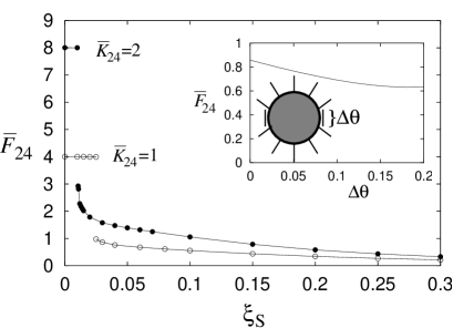
FIG. 15.: The saddle-splay free energy $\overline{F}_{24}$ as a function of $\xi_{S}$ for the same curves as in Fig. 14. Inset: $\overline{F}_{24}$ versus the angular width of the surface ring calculated from the ansatz functions in Eqs. (14) for $\overline{K}_{24}=1$.

et al. clearly demonstrate water droplets dispersed in 5CB do assume the dipole configuration. From the phase diagram we conclude $\xi_{S}<0.09$ as a necessary condition for the existence of the dipole. With $a\approx 1\,\mu\text{m}$, $K_{3}=0.53\times 10^{-6}\,\mathrm{dyn}$, and the definition (21) for $\xi_{S}$ we arrive at

$$W>0.6\,\text{erg}/\text{cm}^{2}\enspace.$$ (39)

If we assume the validity of the Cauchy-Relation (11) which for 5CB gives $\overline{K}_{24}=0.61$, we conclude that $W>1.5\,\text{erg}/\text{cm}^{2}$. Both values indicate one of the highest anchoring strengths ever observed.

FIG. 16.: Phase diagram of the dipole-surface ring transition as a function of $\xi_{S}$ and $\overline{K}_{24}$. Further parameters are indicated in the inset.

IV Conclusions

The purpose of the article was to give a detailed study of the director field around a spherical particle and to illustrate how it can be manipulated by an external field. We clearly find that for large particles and sufficiently strong surface anchoring the dipole is the preferred configuration. For conventional calamitic liquid crystals where $K_{2}<K_{1}$ the dipole should always exhibit a twist around the hyperbolic hedgehog. It should not occur in discotic liquid crystals where $K_{2}>K_{1}$. According to our calculations the bend constant $K_{3}$ only plays a minor role for the twist transition. The Saturn ring appears for sufficiently small particles. However, the dipole can be transformed into the Saturn ring by means of a magnetic field if the Saturn ring is metastable at $H=0$. Otherwise a hysteresis is visible. For the liquid-crystal 5CB we find the Saturn ring to be metastable for a particle size $a=1\,\mu\text{m}$. Increasing the radius $a$ this metastability will vanish in analogy with our calculations within the one-constant approximation (see Fig. 9). Decreasing the surface-anchoring strength $W$ the surface ring configuration with a quadrupolar symmetry becomes absolutely stable. We never find a stable structure with dipolar symmetry where the surface ring has a general angular position $\theta_{d}$ or is even shrunk to a point at $\theta_{d}=0,\pi$. The surface ring is clearly favored by a large saddle-splay constant $K_{24}$.

So far convincing experiments on dispersions of spherical particles in a nematic liquid crystal only exist in the case of inverted nematic emulsions [10, 12, 13]. We hope that the summary of our results stimulates further experiments which try different liquid crystals as a host fluid, manipulate the anchoring strength, investigate the effect of external fields, and attempt to disperse silica or latex spheres [36, 37, 38].

A

For completeness we give the explicit formulas of $\mathchoice{{\hbox{\boldmath$\displaystyle\nabla$}}}{{\hbox{\boldmath$\textstyle\nabla$}}}{{\hbox{\boldmath$\scriptstyle\nabla$}}}{{\hbox{\boldmath$\scriptscriptstyle\nabla$}}}\cdot{\bf n}$, ${\bf n}\cdot\mathchoice{{\hbox{\boldmath$\displaystyle\nabla$}}}{{\hbox{\boldmath$\textstyle\nabla$}}}{{\hbox{\boldmath$\scriptstyle\nabla$}}}{{\hbox{\boldmath$\scriptscriptstyle\nabla$}}}\times{\bf n}$, and ${\bf n}\times(\mathchoice{{\hbox{\boldmath$\displaystyle\nabla$}}}{{\hbox{\boldmath$\textstyle\nabla$}}}{{\hbox{\boldmath$\scriptstyle\nabla$}}}{{\hbox{\boldmath$\scriptscriptstyle\nabla$}}}\times{\bf n})$ for the director field in Eq. (1) and the modified spherical coordinates $(\rho,\theta)$:

$$\mathchoice{{\hbox{\boldmath$\displaystyle\nabla$}}}{{\hbox{\boldmath$\textstyle\nabla$}}}{{\hbox{\boldmath$\scriptstyle\nabla$}}}{{\hbox{\boldmath$\scriptscriptstyle\nabla$}}}\cdot{\bf n}=\sqrt{\rho}(2n_{r}-2\rho n_{r,\rho}+\cot\theta n_{\theta}+n_{\theta,\theta})$$ (A2)

$${\bf n}\cdot\mathchoice{{\hbox{\boldmath$\displaystyle\nabla$}}}{{\hbox{\boldmath$\textstyle\nabla$}}}{{\hbox{\boldmath$\scriptstyle\nabla$}}}{{\hbox{\boldmath$\scriptscriptstyle\nabla$}}}\times{\bf n} = \sqrt{\rho}(2\rho n_{\theta}n_{\phi,\rho}-2\rho n_{\phi}n_{\theta,\rho}-n_{\phi}n_{r,\theta}$$ (A4)

$$+\cot\theta n_{r}n_{\phi}+n_{r}n_{\phi,\theta})$$

$${\bf n}\times(\mathchoice{{\hbox{\boldmath$\displaystyle\nabla$}}}{{\hbox{\boldmath$\textstyle\nabla$}}}{{\hbox{\boldmath$\scriptstyle\nabla$}}}{{\hbox{\boldmath$\scriptscriptstyle\nabla$}}}\times{\bf n}) = \sqrt{\rho}[n_{\theta}(n_{\theta}-2\rho n_{\theta,\rho}-n_{r,\theta})$$ (A10)

$$+n_{\phi}(n_{\phi}-2\rho n_{\phi,\rho})]{\bf e}_{r}$$

$$+\sqrt{\rho}[n_{\phi}(\cot\theta n_{\phi}+n_{\phi,\theta})$$

$$-n_{r}(n_{\theta}-2\rho n_{\theta,\rho}-n_{r,\theta})]{\bf e}_{\theta}$$

$$-\sqrt{\rho}[n_{r}(n_{\phi}-2\rho n_{\phi,\rho})$$

$$+n_{\theta}(\cot\theta n_{\phi}+n_{\phi,\theta})]{\bf e}_{\phi}\enspace.$$

Partial derivatives are indicated by $,i$ ($i=\rho,\theta$) and

$$\frac{\partial}{\partial r}=-2\rho^{3/2}\frac{\partial}{\partial\rho}$$ (A11)

was used.

B Chain rule for functional derivatives

Suppose $F[\Phi_{i}]$ is a functional depending on the fields $\Phi_{i}({\bf x})$ in real space. The functional derivative $\delta F/\delta\Phi_{i}({\bf x})$ is introduced via the Taylor expansion

$$\delta F=F[\Phi_{i}+\delta\Phi_{i}]-F[\Phi_{i}]\approx\sum_{i}\int\frac{\delta F}{\delta\Phi_{i}({\bf x})}\,\delta\Phi_{i}({\bf x})\,d^{3}x\enspace.$$ (B1)

$\delta F$ indicates the change of the functional if at every space point the field $\Phi_{i}({\bf x})$ is changed by the small amount $\delta\Phi_{i}({\bf x})$. The special choice $\delta\Phi_{i}=\delta_{ij}\epsilon\delta({\bf x}-{\bf x}_{0})$ leads directly to the definition

$$\left.\frac{\delta F}{\delta\Phi_{j}({\bf x})}\right|_{{\bf x}={\bf x}_{0}}:=\lim_{\epsilon\rightarrow 0}\frac{F[\Phi_{i}+\delta_{ij}\epsilon\delta({\bf x}-{\bf x}_{0})]-F[\Phi_{i}]}{\epsilon}\enspace.$$ (B2)

If the field $\Phi_{i}$ depends on other fields $\phi_{k}$, i.e., $\Phi_{i}=\Phi_{i}(\phi_{k})$, then with

$$F[\Phi_{i}(\phi_{k}+\delta_{jk}\epsilon\delta({\bf x}-{\bf x}_{0}))] \approx F[\Phi_{i}(\phi_{k})$$ (B4)

$$+\delta_{jk}\epsilon\delta({\bf x}-{\bf x}_{0})\frac{\partial\Phi_{i}}{\partial\phi_{j}}]$$

one obtains immediately the chain rule

$$\frac{\delta F}{\delta\phi_{j}}=\sum_{i}\frac{\delta F}{\delta\Phi_{i}}\,\frac{\partial\Phi_{i}}{\partial\phi_{j}}\enspace$$ (B5)

from Eq. (B2).

REFERENCES

- [1] W. B. Russel, D. A. Saville, and W. R. Schowalter, Colloidal Dispersions (Cambridge University Press, Cambridge, 1995).
- [2] M. Krech, The Casimir Effect in Critical Systems (World Scientific, Singapore, 1994).
- [3] V. M. Mostepanenko and N. N. Trunov, The Casimir effect and its application (Clarendon Press, Oxford, 1997).
- [4] A. D. Dinsmore, A. G. Yodh, and D. J. Pine, Nature 383, 259 (1996).
- [5] A. D. Dinsmore, D. T. Wong, P. Nelson, and A. G. Yodh, Phys. Rev. Lett. 80, 409 (1998).
- [6] D. Rudhardt, C. Bechinger, and P. Leiderer, Phys. Rev. Lett. 81, 1330 (1998).
- [7] F. Brochard and P. G. de Gennes, J. Phys. (Paris) 31, 691 (1970).
- [8] S. Ramaswamy, R. Nityananda, V. A. Raghunathan, and J. Prost, Mol. Cryst. Liq. Cryst. 288, 175 (1996).
- [9] R. W. Ruhwandl and E. M. Terentjev, Phys. Rev. E 55, 2958 (1997).
- [10] P. Poulin, H. Stark, T. C. Lubensky, and D. A. Weitz, Science 275, 1770 (1997).
- [11] T. C. Lubensky, D. Pettey, N. Currier, and H. Stark, Phys. Rev. E 57, 610 (1998).
- [12] P. Poulin, V. Cabuil, and D. A. Weitz, Phys. Rev. Lett. 79, 4862 (1997).
- [13] P. Poulin and D. A. Weitz, Phys. Rev. E 57, 626 (1998).
- [14] R. G. Horn, J. N. Israelachvili, and E. Perez, J. Phys. (Paris) 42, 39 (1981).
- [15] A. Poniewierski and T. Sluckin, Liq. Cryst. 2, 281 (1987).
- [16] I. Muševič, G. Slak, and R. Blinc, Abstract Book p. 91, 16th International Liquid Crystal Conference, Kent, USA, 1996.
- [17] A. Borštnik and S. Žumer, Phys. Rev. E 56, 3021 (1997).
- [18] A. Borštnik, H. Stark, and S. Žumer, submitted to Phys. Rev. E.
- [19] P. Galatola and J. B. Fournier, Abstract Book p. O-19, 17th International Liquid Crystal Conference, Strasbourg, France, 1998.
- [20] A. Ajdari, L. Peliti, and J. Prost, Phys. Rev. Lett. 66, 1481 (1991).
- [21] B. D. Swanson and L. B. Sorenson, Phys. Rev. Lett. 75, 3293 (1995).
- [22] P. Ziherl, R. Podgornik, and S. Žumer, Chem. Phys. Lett. 295, 99 (1998).
- [23] R. B. Meyer, Mol. Cryst. Liq. Cryst. 16, 355 (1972).
- [24] M. V. Kurik and O. D. Lavrentovich, Usp. Fiz. Nauk 154, 381 (1988) [Sov. Phys. Usp. 31, 196 (1988)].
- [25] E. M. Terentjev, Phys. Rev. E 51, 1330 (1995).
- [26] O. V. Kuksenok, R. W. Ruhwandl, S. V. Shiyanovskii, and E. M. Terentjev, Phys. Rev. E 54, 5198 (1996).
- [27] R. W. Ruhwandl and E. M. Terentjev, Phys. Rev. E 56, 5561 (1997).
- [28] P. G. de Gennes and J. Prost, The Physics of Liquid Crystals, 2nd. ed. (Clarendon Press, Oxford, 1993).
- [29] J. Nehring and A. Saupe, J. Chem. Phys. 54, 337 (1971).
- [30] L. M. Blinov, A. Y. Kabayenkov, and A. A. Sonin, Liq. Cryst. 5, 645 (1989).
- [31] M. Kléman, Points, Lines and Walls: In liquid crystals, magnetic systems, and various ordered media (John Wiley & Sons, New York, 1983).
- [32] N. Schopohl and T. J. Sluckin, Phys. Rev. Lett. 59, 2582 (1987).
- [33] E. Penzenstadler and H.-R. Trebin, J. Phys. France 50, 1027 (1989).
- [34] W. H. Press, S. A. Teukolsky, W. T. Vetterling, and B. P. Flannery, Numerical Recipes in Fortran: The Art of Scientific Computing (Cambridge University Press, Cambridge, 1992).
- [35] O. Lavrentovich and E. Terentjev, Zh. Eksp. Teor. Fiz. 91, 2084 (1986) [Sov. Phys. JETP 64, 1237 (1986)].
- [36] P. Poulin, V. A. Raghunathan, P. Richetti, and D. Roux, J. Phys. I France 4, 1557 (1994).
- [37] V. A. Raghunathan, P. Richetti, and D. Roux, Langmuir 12, 3789 (1996).
- [38] V. A. Raghunathan et al., Mol. Cryst. Liq. Cryst. 288, 181 (1996).