[

Dynamical Anomalies and Intermittency in Burgers Turbulence

Abstract

We analyze the field theory of fully developed Burgers turbulence. Its key elements are shock fields, which characterize the singularity statistics of the velocity field. The shock fields enter an operator product expansion describing intermittency. The latter is found to be constrained by dynamical anomalies expressing finite dissipation in the inviscid limit. The link between dynamical anomalies and intermittency is argued to be important in a wider context of turbulence.

PACS numbers: 64.60.Ht, 68.35.Fx, 47.25Cg

]

A field theory of hydrodynamic turbulence is difficult in two ways: It is far from equilibrium and far from the realm of standard perturbative renormalization [1]. New non-perturbative concepts have been established for simpler model systems sharing some characteristics of turbulent fluids. In particular, the stochastic Burgers equation

$$\partial_{t}{\bf v}+({\bf v}\cdot{\bf\nabla}){\bf v}=\nu\,{\bf\nabla}^{2}{\bf v}+{\bf\nabla}\eta$$ (1)

has become an important model for turbulence, recently studied by a variety of methods [2, 3, 4, 5, 6, 7, 8, 9, 10, 11]. It governs the time evolution of a vortex-free velocity field ${\bf v}({\bf r},t)=\nabla h({\bf r},t)$. The equivalent scalar equation

$$\partial_{t}h=\nu\nabla^{2}h+\frac{1}{2}(\nabla h)^{2}+\eta$$ (2)

is known as the Kardar-Parisi-Zhang equation [12, 13]. The driving potential $\eta({\bf r},t)$ is Gauss distributed with mean $\overline{\eta}({\bf r},t)=0$ and correlations

$$\overline{\eta({\bf r},t)\eta({\bf r}^{\prime},t^{\prime})}=\varepsilon r_{0}^{2}\delta(t-t^{\prime})G(|{\bf r}-{\bf r}^{\prime}|/r_{0})$$ (3)

over a characteristic scale $r_{0}$. The function $G$ is taken to be analytic with $G(\rho)=1-G_{2}\rho^{2}+O(\rho^{4})$ and $G_{2}>0$. There is a second characteristic scale, the dissipation length $a_{0}\equiv\nu^{3/4}\varepsilon^{-1/4}$. Burgers turbulence occurs at high values of the Reynolds number $R\equiv(r_{0}/a_{0})^{4/3}$ and shows strong intermittency. For example, the longitudinal velocity difference moments of order $k=2,3,\dots$ take the form

$$\langle[v_{\|}({\bf r}_{1})-v_{\|}({\bf r}_{2})]^{k}\rangle\sim|{\bf r}_{1}-{\bf r}_{2}|^{-kx_{{\bf v}}+\tilde{x}_{k}}\,r_{0}^{-\tilde{x}_{k}}$$ (4)

in the inertial scaling regime $r_{0}/R\ll|{\bf r}_{1}-{\bf r}_{2}|\ll r_{0}$ [3, 4]. The third moment grows linearly with $|{\bf r}_{1}-{\bf r}_{2}|$, i.e., $x_{\bf v}=-1/3$ and $\tilde{x}_{3}=0$. The other moments, however, acquire a singular dependence on $r_{0}$, which defines the intermittency exponents $\tilde{x}_{k}$. The turbulent state is associated with a particular strong-coupling limit of Eq. (1), called the turbulent limit in the sequel: $\nu\to 0$ at fixed driving given by (3). In that limit, the velocity field acquires discontinuities called shocks (see Fig. 1). It is these singularities that cause intermittency.

Burgers’ equation has a number of further applications. It has been proposed as a model for galaxy formation [14]. The Kardar-Parisi-Zhang equation (2) models stochastic surface growth described by the “height” field $h({\bf r},t)$, and is related to directed polymers in a quenched random medium. In these contexts, the driving force is usually taken to be random in time and space,

$$\overline{\eta({\bf r},t)\eta({\bf r}^{\prime},t^{\prime})}=\gamma^{2}\delta(t-t^{\prime})\delta({\bf r}-{\bf r}^{\prime})\;.$$ (5)

For $\nu^{3}/\gamma^{2}\to 0$, there is again a strong coupling limit, which, however, is quite different from the turbulent limit. The scaling is probably non-intermittent,

$$\langle(h({\bf r}_{1})-h({\bf r}_{2}))^{k}\rangle\sim|{\bf r}_{1}-{\bf r}_{2}|^{-kx_{h}}\;.$$ (6)

The exponent $x_{h}$ depends on the dimension $d$. The value $x_{h}=-1/2$ for $d=1$ is well-known [15], while $x_{h}=-2/5$ for $d=2$ has been obtained only recently [16, 13].

This Letter studies the field theory of stationary Burgers turbulence. The basic quantities of this field theory are scaling fields containing powers of the local velocity ${\bf v}$ and its gradients, $\nabla{\bf v}$, $\nabla\nabla{\bf v}$, etc. In particular, the statistics of the shocks is represented by a family of renormalized shock fields $\Sigma_{k}$ ($k=1,2,\dots$) that remain finite in the turbulent limit. Another family of fields $s_{k}$ describes velocity gradients away from shocks. The short-distance properties of the scaling fields are encoded in an operator product expansion (OPE). This is a familiar concept in field theory (see, e.g., ref. [17]). It has recently been

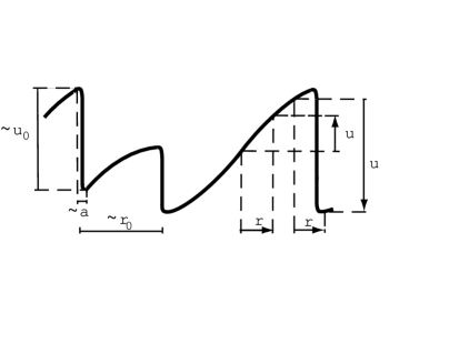
FIG. 1.: Stationary Burgers turbulence in one dimension. The velocity profile $v(r,t)$ at a given time $t$ is an ensemble of shocks with amplitude $\sim u_{0}$, width $\sim a$, and mutual distance $\sim r_{0}$. The probability distribution $P_{r}(u)$ of the longitudinal velocity difference over a distance $a\ll r\ll r_{0}$ is generated by no-shock and single-shock configurations (lines with arrows).

extended to non-equilibrium systems. OPEs have been proposed for general turbulent systems by Adzhemyan, Antonov, and Vasil’ev [18], Eyink [19] (see also Duplantier and Ludwig [20]), and by L’vov and Procaccia [21], for Burgers turbulence by Polyakov [5], and for the Kardar-Parisi-Zhang equation by Lässig [16]. The Burgers OPE discussed here differs from Polyakov’s conjecture by the explicit inclusion of the fields $\Sigma_{k}$ and $s_{k}$. It is an important tool to understand the dynamics of Burgers turbulence. The shock singularities preventing a straightforward evaluation of the equation of motion, the stationary state is maintained by a rather subtle balance of driving forces, convection, and dissipation. We discuss the resulting distribution of velocity differences (the functional form of which has been much debated [3, 4, 5, 6, 7, 8, 9, 10, 11]), as well as the flux of the energy density and its generalizations. The energy dissipated per unit of volume and time remains finite in the turbulent limit $\nu\to 0$. In the field theory of Burgers’ equation, this is reflected by dynamical anomalies, i.e., asymptotically finite dissipation terms in effective equations of motion for the inertial regime. These are associated with conservation laws that are valid for the inviscid equation without driving ($\nu=0$, $\varepsilon=0$) but are broken in the driven state at any finite $\nu$ [22, 5]. We find anomalies given by operator products involving the shock fields. This is not surprising since dissipation takes place at the shocks. Dynamical anomalies and intermittency are indeed closely related: they are both generated by the singularities of the velocity field. This conceptual link and the underlying theoretical framework are expected to extend to other turbulent systems, as we briefly discuss at the end of this Letter.

The basic phenomenology of stationary Burgers turbulence is well established in one dimension [3, 10] but appears to be much the same in higher dimensions [4, 6]. The velocity profile ${\bf v}({\bf r},t)$ at a given time $t$ looks similar to that of decaying Burgers turbulence with random initial data [23, 24, 25]. It consists of ramps (i.e., regions where the velocity derivatives $\nabla{\bf v}$, $\nabla\nabla{\bf v}$, etc. are finite) separated by shock singularities, as sketched in Fig. 1. Shocks develop out of ramp regions through preshock singularities (which have the cubic root form $v({\bf r})-v({\bf r}_{\rm ps})\sim-(\epsilon({\bf r}-{\bf r}_{\rm ps}))^{1/3}$ for $d=1$ [9]). The shocks have amplitudes of order $u_{0}\equiv(\varepsilon r_{0})^{1/3}$ and distances of order $r_{0}$ to their neighbors; the slopes of the ramps are of order $u_{0}/r_{0}$. These scales are independent of $\nu$, while the typical shock width $a\equiv r_{0}/R=\nu/u_{0}$ vanishes in the turbulent limit. From these shock characteristics, the velocity statistics can be inferred in an approximate way that appears to give the correct scaling. Consider, for example, the longitudinal velocity difference $u\equiv v_{\|}({\bf r}_{1},t)-v_{\|}({\bf r}_{2},t)$ (with $v_{\|}\equiv{\bf v}\cdot({\bf r}_{1}-{\bf r}_{2})/r$ and $r\equiv|{\bf r}_{1}-{\bf r}_{2}|$) and the local excess velocity ${\bf w}({\bf r},t)\equiv{\bf v}({\bf r},t)-\langle{\bf v}\rangle$. These have normalized probability distributions $P_{r}(u){\rm d}u$ and $Q({\bf w}){\rm d}^{d}{\bf w}$, respectively. $Q({\bf w})$ depends only on the absolute value $|{\bf w}|$ by rotational invariance and parity but $P_{r}(u)$ is an asymmetric function of $u$ since the dynamics is not invariant under the transformation ${\bf v}\to-{\bf v}$. Both distributions are invariant under Galilei transformations ${\bf v}({\bf r},t)\to{\bf v}({\bf r}-{\bf v}_{0}t,t)-{\bf v}_{0}$. In the turbulent limit, they are independent of $\nu$, i.e., of the shock width $a$. Hence, they can be written in scaling form,

$$P_{r}(u)=\frac{1}{u_{r}}\,{\cal P}\!\left(\frac{u}{u_{r}},\frac{r}{r_{0}}\right),\;\;\;Q({\bf w})=\frac{1}{u_{0}^{d}}\,{\cal Q}\!\left(\frac{|{\bf w}|}{u_{0}}\right),$$ (7)

where $u_{r}\sim u_{0}r/r_{0}$ is the average velocity increment over a distance $r$ on a ramp. By Eq. (7), the single-point moments scale in a simple way,

$$\langle|{\bf w}|^{k}\rangle\sim u_{0}^{k}\sim r_{0}^{-x_{k}}\;,\;\;\;x_{k}=-k/3\;.$$ (8)

For $\rho\equiv r/r_{0}\ll 1$, the powers of the velocity difference can be expanded in the number of shocks present between ${\bf r}_{1}$ and ${\bf r}_{2}$. One obtains $u^{k}\sim p_{0}u_{r}^{k}+p_{1}u_{0}^{k}+O(p_{2})$ with the $n$-shock probabilities $p_{0}\simeq 1-\rho$, $p_{1}\simeq\rho+O(\rho^{2})$, $p_{n}=O(\rho^{n})$ . This implies the bifractal moments [3, 4]

$$\langle u^{k}\rangle\sim\left\{\begin{array}[]{ll}u_{r}^{k}\sim r^{k}r_{0}^{-2k/3}&\;\;(k<1)\\ (r/r_{0})u_{0}^{k}\sim rr_{0}^{(k-3)/3}&\;\;(k>1)\end{array}\;.\right.$$ (9)

What does all this mean for the field theory of the turbulent state? Correlation functions in the inertial regime should be represented by a field theory with short-distance cutoff $a$. Scale invariance emerges in the turbulent continuum limit $a\to 0$. Since that limit is nonsingular for velocity correlations, the scaling dimension of the field ${\bf v}({\bf r},t)$ takes the Kolmogorov value $x_{\bf v}=-1/3$; the fields ${\bf v}^{k}({\bf r},t)$ have dimensions $x_{k}=kx_{\bf v}$ ($k=1,2,\dots)$. Indeed, the distributions (7) and the resulting moments (8), (9) are covariant under the scale transformations ${\bf r}\to b{\bf r}$, $r_{0}\to br_{0}$, ${\bf v}\to b^{x_{\bf v}}{\bf v}$ at fixed $\varepsilon$. Turbulence does generate short-distance singularities for the moments of velocity gradients. Defining the longitudinal gradient $\nabla\cdot{\bf v}\equiv u/r$ with a discretization length $r\sim a$, we write

$$(\nabla\cdot{\bf v})^{k}({\bf r},t)=Z_{k}^{-1}\Sigma_{k}({\bf r},t)+s_{k}({\bf r},t)\;.$$ (10)

The fields $\Sigma_{k}({\bf r},t)$ and $s_{k}({\bf r},t)$ represent the contributions from configurations with and without a shock in the discretization interval. Using Eq. (9), we have

$$Z_{k}^{-1}\langle\Sigma_{k}\rangle \sim \frac{u_{0}^{k}}{a^{k-1}r_{0}}\sim\frac{r_{0}^{-\tilde{x}_{k}}}{a^{k-1}}\;,\;\;\;\tilde{x}_{k}=-\frac{k-3}{3}\;,$$ (11)

$$\langle s_{k}\rangle_{\rm reg} \sim (u_{0}/r_{0})^{k}\sim r_{0}^{-x^{\prime}_{k}}\;,\;\;\;x^{\prime}_{k}=2k/3\;.$$ (12)

The multiplicative renormalization factors $Z_{k}\sim a^{k-1}$ absorb the short-distance singularities in (11), which defines the cutoff-independent fields $\Sigma_{k}$ of dimension $\tilde{x}_{k}$. The slope fields $s_{k}$ have different dimensions $x_{k}^{\prime}$ determined by the regular part (12) of the ramp slope moments.

We now make the assumption that the velocity field satisfies an OPE of the form

$${\bf v}({\bf r}_{1})\dots{\bf v}({\bf r}_{k}) = r^{-kx_{\bf v}+\tilde{x}_{k}}\,C_{k}\,\Sigma_{k}({\bf r}_{1})+$$ (14)

$$r^{-kx_{\bf v}+x_{k}^{\prime}}\,c_{k}\,s_{k}({\bf r}_{1})+\dots$$

with $r\equiv|{\bf r}_{1}-{\bf r}_{2}|$. Both sides of this relation are tensors of rank $k$ whose indices are suppressed. The right hand side is a sum over all local scaling fields. The displayed terms contain the lowest-dimensional Galilei-invariant fields representing shock and ramp configurations, respectively, multiplied by dimensionless coefficient functions $C_{k}({\bf r}_{12}/r,\dots,{\bf r}_{1k}/r)$ and $c_{k}({\bf r}_{12}/r,\dots,{\bf r}_{1k}/r)$ (simple numbers for $k=2$), and powers of $r$ as required by dimensional analysis. The suppressed terms involve subleading Galilei-invariant fields and noninvariant fields such as ${\bf v}^{k}$, $\nabla{\bf v}^{k}$, etc. By differentiating (14), one obtains a manifestly Galilei-invariant OPE for velocity gradients,

$$\nabla\cdot{\bf v}({\bf r}_{1})\dots\nabla\cdot{\bf v}({\bf r}_{k}) \sim \prod_{i=2}^{k}\delta({\bf r}_{i}-{\bf r}_{i-1})\Sigma_{k}({\bf r}_{1})+$$ (16)

$$s_{k}({\bf r}_{1})+\dots\;;$$

see also [19] for general turbulent systems. Here the shock fields generate only contact singularities, while the slope fields have regular coefficients. It is not known whether there are other singular terms.

The OPE is a consistency condition between renormalized correlation functions in the stationary state. It relates, for example, the $n$-point function $\langle{\bf v}({\bf r}_{1})\dots{\bf v}({\bf r}_{n})\rangle$ to the $(n-k+1)$-point functions $\langle\Sigma_{k}({\bf r}_{1}){\bf v}({\bf r}_{k+1})\dots{\bf v}({\bf r}_{n})\rangle$ and $\langle s_{k}({\bf r}_{1}){\bf v}({\bf r}_{k+1})\dots{\bf v}({\bf r}_{n})\rangle$ in the limit $a\ll|{\bf r}_{ij}|\ll|{\bf r}_{il}|,r_{0}$ ($i,j=1,\dots,k$ and $l=k+1,\dots,n$). The coefficient functions $C_{k}$ etc. are assumed to describe local properties of the inertial regime independent of the cutoffs $a$ and $r_{0}$. Hence, the existence of an OPE embodies two important characteristics of the turbulent field theory: (i) It is renormalized, i.e., the short-distance singularities of all scaling fields have been removed in a consistent way. (ii) The large-distance singularities are created solely by the single-point amplitudes of negative-dimensional fields, $\langle{\cal O}\rangle\sim r_{0}^{-x_{\cal O}}$. In particular, the intermittency exponent $\tilde{x}_{k}$ in Eq. (4) equals the scaling dimension of the leading Galilei-invariant field in the expansion (14). This is indeed the case for Burgers turbulence, where $\langle u^{k}\rangle\sim\langle\Sigma_{k}\rangle\sim r_{0}^{-\tilde{x}_{k}}$ with $\tilde{x}_{k}=-(k-3)/3$ according to Eqs. (9) and (11).

The OPE (14) has important consequences for Burgers dynamics, which we now discuss for simplicity in $d=1$. For purely convective dynamics ($\nu=0$, $\varepsilon=0$), the moments of the excess velocity $w^{k}({\bf r},t)$ are locally conserved, $\partial_{t}w^{k}+(k/(k+1))\nabla(w^{k+1})=0$ ($k=1,2,\dots$). In the driven state, $\langle w^{k}({\bf r},t)\rangle$ is pumped with a finite rate $\varepsilon\langle\partial_{w}^{2}w^{k}({\bf r},t)\rangle\sim r_{0}^{-x_{k-2}}$ ($k=2,4,\dots$). This cannot be offset by convection since $\langle\nabla(w^{k+1})({\bf r},t)\rangle=0$. Hence, the stationary state must be maintained by a dynamical anomaly [5],

$$\varepsilon\langle\partial_{w}^{2}w^{k}({\bf r})\rangle+\nu\langle(\nabla^{2}w)({\bf r})\,\partial_{w}w^{k}({\bf r})\rangle=0\;.$$ (17)

It is easy to check that the OPE (14) predicts the correct form of the anomaly. We have

$$\nu\langle(\nabla^{2}w)({\bf r})\,w^{k-1}({\bf r})\rangle \sim \nu\delta(0)\,\langle s_{k}({\bf r})\rangle$$ (18)

$$\sim r_{0}^{-\tilde{x}_{k}+1/3}\sim r_{0}^{-x_{k-2}}\;,$$ (19)

using $\nu\sim a_{0}^{4/3}\sim ar_{0}^{1/3}$ and a regularization on the scale of the short-distance cutoff, $\delta(0)\sim a^{-1}$. Hence, the OPE and the resulting anomalies provide a link between the fields $v^{k}$ and the shock fields $\Sigma_{k}$. This fixes the intermittency exponents by the scaling relations $\tilde{x}_{k}=x_{k-2}+1/3$ in accordance with (8) and (11).

The role of dissipation is more subtle for the velocity differences. Consider again the shock number expansion $P_{r}(u)=(1-\rho)P_{r}^{0}(u)+\rho P_{r}^{1}(u)+O(\rho^{2})$ for $\rho\ll 1$. By virtue of the OPE (14), the equation of motion for the conditional distributions $P_{r}^{0}(u)$ and $P_{r}^{1}(u)$ is then essentially reduced to that of the families of single-point amplitudes $\langle\Sigma_{k}\rangle$ and $\langle s_{k}\rangle_{\rm reg}$, respectively.

1. The zero-shock part $P^{0}_{r}(u)$ is also covariant under the ‘convective’ scale transformations $r\to br$, $u\to bu$ at fixed $\varepsilon$ and $r_{0}$ and can hence be written in the scaling form $P_{r}^{0}(u)=(1/u_{r}){\cal P}^{0}(u/u_{r})$ discussed in [5]. In other words, the expansion $u^{k}=r^{k}s_{k}+(1/2)r^{k+1}\nabla s_{k}+\dots$ is dominated by the first term, which depends on the large-distance scale $r_{0}$ only through the ramp slope moment $\langle s_{k}\rangle\sim(u_{0}/r_{0})^{k}$. The convective symmetry is expected to be broken for $-u\,\raisebox{-2.58334pt}{$\stackrel{{\scriptstyle>}}{{\displaystyle{\sim}}}$}\,\tilde{u}_{r}\equiv(\epsilon r)^{1/3}$ by curvature effects at preshocks. This is precisely the scale where $P_{r}(u)$ becomes dominated by the shock part; see (20) below. In the equation of motion for ${\cal P}^{0}$, dissipation can be neglected at all points of finite $\nabla^{2}v$ (and even at preshocks). Furthermore, driving and convection are local processes in velocity space. It is straightforward to show that they are represented by the differential operators $G_{2}\partial_{\omega}^{2}{\cal P}^{0}(\omega)$ and $(\partial_{\omega}\omega^{2}+\omega){\cal P}^{0}(\omega)$, respectively [5, 10]. In particular, the term $\omega{\cal P}^{0}(\omega)$ describes a change in measure due to convective squeezing or stretching of the ramps [10]. We will be interested in solutions with a positive average ramp slope, i.e., with a net gain in measure, $\langle\omega\rangle>0$. The formation of shocks, on the other hand, produces a measure loss $L(\omega)<0$. In the stationary state, the net loss offsets the convective gain, $\langle\omega\rangle+\langle L(\omega)\rangle=0$. For consistency with known properties of $P_{r}(u)$, the equation of motion $(G_{2}\partial_{\omega}^{2}+\partial_{\omega}\omega^{2}+\omega+L){\cal P}^{0}=0$ must have a normalized, positive solution which behaves asymptotically as ${\cal P}^{0}\sim\omega\exp(-\omega^{3}/3G_{2})$ for $\omega\gg 1$ [6, 9] and ${\cal P}^{0}\sim|\omega|^{-3-\alpha}$ for $\omega\ll-1$, with $\alpha\geq 0$, most likely $\alpha=1/2$ [9]. This requires $L(\omega)=o(\omega)$ for $\omega\gg 1$ and $L(\omega)\simeq\alpha\omega$ for $\omega\ll-1$. The ‘anomaly’ $L(\omega)$ can be associated with ultraviolet-finite operator products $\Sigma_{1}(r)s_{k}(r)$ [26]. It is not clear, however, whether the functions $L(\omega)$ and, hence, ${\cal P}^{0}(\omega)$ are entirely determined by the OPE.

2. The single-shock part $P^{1}_{r}(u)$ is expected to have the scaling form $P_{r}^{1}(u)=(\rho/u_{0}){\cal P}^{1}(-u/u_{0})+O(\rho^{2})$. The leading term depends on $r$ only through the shock probability $p_{1}\simeq\rho$ in accordance with the OPE (14) and the moments (9). ${\cal P}^{1}(\sigma)$ is the scaled shock size distribution function. The equation of motion for a single shock produces a driving term $\partial_{\sigma}^{2}{\cal P}^{1}(\sigma)$ and a convection term $\partial_{\sigma}f(\sigma)\sigma{\cal P}^{1}(\sigma)$, while dissipation can again be neglected. Here $(u_{0}/r_{0})f(\sigma)$ is the expectation value of the average ramp slope to both sides of a shock of size $u_{0}\sigma$. For very large shocks ($\sigma\gg 1$), this will be positive and proportional to the shock size, leading to the asymptotic equation of motion [27] $(\partial_{\sigma}^{2}+A\partial_{\sigma}\sigma^{2}){\cal P}^{1}=0$ with a constant $A>0$. This determines the tail of the shock size distribution, ${\cal P}^{1}\sim\exp(-A\sigma^{3}/3)$ for $\sigma\gg 1$, in agreement with instanton calculations [7], while the dynamics of initial shock growth suggests ${\cal P}^{1}\sim\sigma$ for $\sigma\ll 1$ [11].

The distribution $P_{r}(u)$ should be dominated by the zero-shock part for small velocity differences $|u|\sim u_{r}$ and by the single-shock part for large negative values $u\sim-u_{0}$. The crossover scale $-\tilde{u}_{r}=-u_{r}\rho^{-2/3}$ is obtained by matching the two expressions, $P_{r}^{0}(-\tilde{u}_{r})\sim\rho P_{r}^{1}(-\tilde{u}_{r})$. Thus we conjecture, using the scaling form of Eq. (7),

$${\cal P}(\omega,\rho)\simeq\left\{\begin{array}[]{ll}{\cal P}^{0}(\omega)&\;\;(\omega\rho^{2/3}\raisebox{-2.58334pt}{$\stackrel{{\scriptstyle>}}{{\displaystyle{\sim}}}$}-1)\\ \rho^{2}{\cal P}^{1}(-\omega\rho)&\;\;(\omega\rho^{2/3}\raisebox{-2.58334pt}{$\stackrel{{\scriptstyle<}}{{\displaystyle{\sim}}}$}-1)\end{array}\right.\;.$$ (20)

It is easy to verify that this solution is indeed normalizable and has the correct moments (9). It has $\langle u\rangle>0$ over ramps and $\langle u\rangle<0$ at shocks, which is compatible with the constraint $\langle u\rangle=0$ due to translational invariance.

To summarize: Burgers field theory contains two different families of local scaling fields, $\Sigma_{k}$ and $s_{k}$, which represent powers of singular and regular velocity gradients, respectively. The fields $\Sigma_{k}$ live on the shocks; their amplitudes $\langle\Sigma_{k}\rangle$ generate intermittency. They are coupled to the other scaling fields through an OPE. The resulting dynamical anomalies fix the intermittency exponents through scaling relations. The anomalies for velocity differences have a simple physical cause: the formation of singular velocity configurations out of regular ones.

How much of this framework is preserved in Navier-Stokes turbulence can only be conjectured at present. Intermittency is still created by the infrared-divergent one-point amplitudes of negative-dimensional Galilei-invariant fields. These are associated with the singularities of the turbulent flow. Vortex filaments, for example, could play the role of the Burgers shocks [1]. The singularities have a much more complicated statistics, however. They lead to multifractal instead of bifractal scaling and may indeed suppress a coherent convective scaling regime $P_{r}(u)\simeq(1/u_{r}){\cal P}^{0}(\omega)$. A stronger breakdown of convective symmetry may produce anomalies and, hence, scaling relations compatible with intermittency exponents $\tilde{x}_{k}$ nonlinear in $k$. Will such relations actually determine the values of $\tilde{x}_{k}$, leading to a nonperturbative theory of turbulence?

I thank Victor Yakhot for useful discussions.

REFERENCES

- [1] See, for example, U. Frisch, Turbulence, Cambridge University Press (1995).
- [2] Ya. Sinai, J. Stat. Phys. 64, 1 (1994).
- [3] A. Chekhlov and V. Yakhot, Phys. Rev. E 52, 5681 (1995); Phys. Rev. Lett. 77, 3118 (1995).
- [4] J.-P. Bouchaud, M. Mézard, and G. Parisi, Phys. Rev. E 52, 3656 (1995); J.-P. Bouchaud and M. Mézard, Phys. Rev. E 54, 5116 (1996).
- [5] A.M. Polyakov, Phys. Rev E 52, 6183 (1995).
- [6] V. Gurarie and A. Migdal, Phys. Rev. E 54, 4908 (1996).
- [7] E. Balkovsky et al., Phys. Rev. Lett. 78, 1452 (1997); Int. J. of Mod. Phys. B 11, 3223 (1997).
- [8] S. Boldyrev, Phys. Rev. E 55, 6907 (1997); Phys. Plasmas 5, 1681 (1998).
- [9] W. E et al., Phys. Rev. Lett. 78, 1904 (1997); W. E and E. vanden Eijnden, Phys. Rev. Lett. 83, 2572 (1999); e-print chao-dyn/9904028.
- [10] T. Gotoh and R.H. Kraichnan, Phys. Fluids 10, 2859 (1998); R.H. Kraichnan, Phys. Fluids 11, 3738 (1999).
- [11] J. Bec, U. Frisch, and K. Khanin, e-print chao-dyn/9910001.
- [12] M. Kardar, G. Parisi, and Y.-C. Zhang, Phys. Rev. Lett. 56, 889 (1986).
- [13] For a recent review, see M. Lässig, J. Phys. C 10, 9905 (1998), also as e-print cond-mat/9806330.
- [14] Ya. Zeldovich, Astron. Astrophys. 5, 84 (1972).
- [15] D. Forster, D.R. Nelson, and M. Stephen, Phys. Rev. A 16, 732 (1977).
- [16] M. Lässig, Phys. Rev. Lett. 80, 2366 (1998).
- [17] See, e.g., J.L. Cardy, Scaling and Renormalization in Statistical Physics, Cambridge University Press (1996).
- [18] L.Ts. Adzhemyan, N.V. Antonov, and A.N. Vasil’ev, Sov. Phys. JETP 68, 733 (1989), Phys. Usp. 39, 1193 (1996).
- [19] G. Eyink, Phys. Lett. A 172, 355 (1993); Chaos, Solitons & Fractals 5, 1465 (1995).
- [20] B. Duplantier and A. Ludwig, Phys. Rev. Lett. 66, 247 (1991).
- [21] V. L’vov and I. Procaccia, Phys. Rev. Lett. 76, 2898 (1996); Phys. Rev E 54, 6268 (1996).
- [22] V. Gurarie, in Recent progress in statistical mechanics and quantum field theory, Los Angeles (1994).
- [23] S. Kida, J. Fluid Mech. 93, 337 (1979).
- [24] Z.-S. She, E. Aurell, and U. Frisch, Commun. Math. Phys. 148, 623 (1992).
- [25] S.N. Gurbatov et al., J. Fluid Mech. 344, 339 (1997).
- [26] The leading term for is given by the operator product . The subleading terms, however, involve the scale explicitly. Polyakov’s OPE [5, 8] contains only the families of ultraviolet-finite fields and , or equivalently, the generating fields and . In terms of these fields, the anomaly cannot be represented by local operator products.
- [27] Both approximations neglect shock-shock interactions, which are important at intermediate values of .