Anomalous transport in normal-superconducting and ferromagnetic-superconducting nanostructures

Abstract

We have calculated the temperature dependence of the conductance variation ($\delta S(T)$) of mesoscopic superconductor normal metal(S/N) structures, in the diffusive regime, analysing both weak and strong proximity effects. We show that in the case of a weak proximity effect there are two peaks in the dependence of $\delta S(T)$ on temperature. One of them (known from previous studies) corresponds to a temperature $T_{1}$ of order of the Thouless energy ($\epsilon_{Th}$), and another, newly predicted maximum, occurs at a temperature $T_{2}$ where the energy gap in the superconductor $\Delta(T_{2})$ is of order $\epsilon_{Th}$. In the limit $L_{\phi}<L$ the temperature $T_{1}$ is determined by $D\hbar/L^{2}_{\phi}$ ($L_{\phi}$ is the phase breaking length), and not $\epsilon_{Th}$. We have also calculated the voltage dependence $\delta S(V)$ for a S/F structure (F is a ferromagnet) and predict non-monotonic behaviour at voltages of order the Zeeman splitting.

Since the late 1970’s it has been known that the conductance ($G$) of S/N mesoscopic structures depends on temperature ($T$) (and voltage ($V$)) in a non-monotonic way (see reviews [1, 2]). This behaviour was first predicted in Ref. [3] where a simple point S/N contact was analysed. The authors of Ref. [3], using a microscopic theory and assuming that the energy gap in the superconductor ($\Delta$) is much less than the Thouless energy $\epsilon_{Th}\equiv\hbar D/L^{2}$ ($D$ is the diffusion constant), showed that the zero-bias conductance $G$ coincides at zero temperature with its normal state value ($G_{n}$). With increasing $T$, $G$ exhibits a non-monotonic behaviour, increasing to a maximum of $G_{max}\approx 1.25G_{n}$ at $T_{m}\approx\Delta(T_{m})$ and then decreasing to $G_{n}$ for $T>T_{m}$.

Recently mesoscopic S/N structures have been fabricated in which the limit $\Delta>>\epsilon_{Th}$ is realised. In this case Nazarov and Stoof [4] (also see [5, 6, 7]) argued that the temperature dependence of the conductance $G$ has a similar non-monotonic behaviour with a maximum at a temperature comparable with the Thouless energy, while simultaniously Volkov, Allsopp and Lambert [8] predicted that the voltage dependence of the conductance in an S/N mesoscopic structure (Andreev interferometer) has a similar form with a maximum at $eV_{m}\approx\epsilon_{Th}$. This non-monotonic behaviour has been observed both in very short S/N contacts [9] and in longer mesoscopic S/N structures [10, 11, 12, 21]. In ref [6] it was noted that the conductance $\delta G=G-G_{n}$ consists of two contributions. The first, $\delta G_{DOS}$, is negative due to a proximity effect induced decrease in the density of states (DOS) of the normal wire which makes contact with a superconducting strip [13]. The other contribution $\delta G_{MT}$ (positive) is analogous to the Maki-Thompson (MT) contribution to the paraconductivity of S/N/S and N/S/N mesoscopic structures and was calculated in [14]. At $T=0$ and $V=0$ both contributions to the conductance are equal, as $T$ or $V$ increase the contribution $\delta G_{MT}$ dominates until a maximum is reached, then both these contributions decay.

During the past decade a great deal of interest in the transport properties of N/S nanostructures has originated from a desire to use superconductivity as a probe into phase-coherent transport. Indeed the above experiments reveal little about the superconductor itself, since the non-monotonic behaviour occurs at an energy much lower than $\Delta(0)$. In this paper we calculate the conductance of mesoscopic S/N structures (see Fig. 1) over a wide temperature range ($0<T\leq T_{c}$), and show that in the dependence of $\delta G(T)$, a second maximum may appear near $T_{c}$ when $\Delta(T_{m})$ is of order the Thouless energy. Consequently, in contrast with non-monotonic phenomena studied to-date, this peak provides a novel quasi-particle transport probe for the energy gap of the superconductor. Indeed we show later that this second maximum is very sensitive to the damping rate inside the superconductor.We also show that if the depairing rate $\gamma$ (for example, due to magnetic impurities) is not small compared to $\epsilon_{Th}$ then the maxima in $\delta G(T)$ occur at a temperature $T_{1}\approx\gamma$ and $\Delta(T_{1})\approx\gamma$.

We consider S/N mesoscopic structures of the form shown in Fig. 1A and 1B. Although they differ slightly from each other, in the limit $l_{1}<<1$ ($l_{1}=L_{1}/L$) the formulae for the conductances of these systems are identical. We assume the metals are diffusive and employ the well developed quasiclassical Green’s function technique (see for example [15]) which has been widely used for studying transport phenomena in S/N mesoscopic structures [2, 3, 4, 5, 6, 8, 16, 17, 18, 19, 7, 20, 21]. Using the Keldysh formalism, the conductance variation of the structure shown in Fig. 1B is given by [17],

$$\delta S=\int^{\infty}_{0}d\epsilon\beta F_{v}^{\prime}(\epsilon)\frac{t(\epsilon)}{1-t(\epsilon)}$$ (1)

where all the quantites are dimensionless (dimensional quantities will be denoted by a tilde); $\delta S=(G-G_{n})/G_{n},\beta=(2T)^{-1},F_{v}^{\prime}(\epsilon)=[\cosh^{-2}\left(\epsilon+eV\right)\beta$ $+\cosh^{-2}\left(\epsilon-eV\right)\beta]/2$, $t(\epsilon)=<\tanh^{2}\left(Re(u(\epsilon,x)\right))>,<A>=(1-l_{1})^{-1}\int^{1}_{l_{1}}dxA$. All energies and voltages are measured in units of the Thouless energy ($\epsilon_{Th}$), the function $u(\epsilon,x)$ is related to the condensate and normal Green’s functions: $F^{R(A)}=\sinh(u^{R(A)}),G^{R(A)}=\cosh(u^{R(A)})$, which obey the Usadel equation,

$$\partial^{2}_{xx}u^{R(A)}-(k^{R(A)})^{2}\sinh u^{R(A)}=0$$ (2)

where $(k^{R(A)})^{2}=\gamma\mp 2i\epsilon$. Eq. (2) can be solved numerically [4, 5], and in some limiting cases analytically [3, 4, 5, 6, 8, 16, 17, 18, 19, 7, 20, 21].

First we consider the simplest case, where the proximity effect is weak, this occurs when the condensate function in the N wire $F^{R(A)}$ is small ($|F^{R(A)}|\approx u^{R(A)}<<1$) [6, 8]. In this limit Eqs. (1) and (2) can be linearized. Also if the length $L$ is longer than the phase breaking length (if $\gamma>>1$) then the N wire may be considered as infinitely long, thus the solution to Eq.(2) is determined by the expression [18],

$$\tanh(u/4)=\tanh(u_{0}/4)e^{-kx}$$ (3)

where $u_{0}$ is determined by the boundary condition at the S/N interface. In the case of a good contact at the $N/N^{\prime}$ interface the function $u$ should be zero at this interface ($x=1$), whereas Eq. (3) gives a nonzero value for $u(\epsilon,1)$. The correction to the solution (3) is small provided that $\gamma>>1$. In the case of the weak proximity effect we solve the linearized form of Eq (1) with the boundary condition at the S/N interface [2],

$$r_{b}\partial_{x}\hat{F}^{R(A)}=-\hat{F}^{R(A)}_{s}|_{x=0}$$ (4)

where $r_{b}$ is the ratio of the S/N interface resistance to the resistance of the N wire of length $L$; $\hat{F}^{R(A)}_{s}=i\hat{\sigma}_{y}F^{R(A)}_{s}\cos(\phi/2)$ is the condensate Green’s function in the superconductor, $F^{R(A)}_{s}=\Delta/\sqrt{(\epsilon\pm i\Gamma)^{2}-\Delta^{2}}$, $\Gamma$ is the damping rate in the spectrum of the superconductor and $\phi$ is the phase difference between the superconductors. In the case of zero $N/N^{\prime}$ interface resistance the condensate function $F^{R(A)}$ (or $u^{R(A)}$) must equal zero when $x=1$. The solution is

$$\hat{F}^{R(A)}\approx i\hat{\sigma}_{y}u^{R(A)}=\frac{\hat{F}^{R(A)}_{s}\sinh(k^{R(A)}(1-x))}{r_{b}(k\cosh k)^{R(A)}}$$ (5)

The proximity effect is weak provided that $r_{b}\sqrt{\Gamma}>>1$ (a maximal value of $F^{R(A)}$ is achieved at $\epsilon=\Delta$). In this case the function $t(\epsilon)$ can be presented in the form [6]:$t(\epsilon)=1/4<(F^{R}-F^{A})^{2}>$. Performing the spatial averaging we obtain in the limit $l_{1}<<1$,

$$\begin{array}[]{cc}t(\epsilon)=(2r_{b})^{-2}(\frac{|F_{s}|^{2}}{|k\cosh k|^{2}}[\frac{\sinh 2k_{1}}{2k_{1}}-\frac{\sin 2k_{2}}{2k_{2}}]\\ +Re(\frac{F_{s}^{2}}{(k\cosh k)^{2}}[\frac{\sinh(2k)}{2k}-1])\cos^{2}(\phi/2)\end{array}$$ (6)

where $k=k_{1}+ik_{2}$. The first term in Eq. (6) represents the anomalous MT contribution to the conductance variation and the second regular term is due to a DOS variation of the N wire caused by the proximity effect. One can easily check that the $partial$ conductance variation $t(\epsilon)$ is zero at $\epsilon=0$ (in this case $F^{R}=F^{A}$), increases as $\epsilon^{2}$, reaching the first maximum when $\epsilon$ is of order max[1,$\gamma$] then decreases. At $\epsilon\approx\Delta$ the function $t(\epsilon)$ has a second maximum (see solid line in Fig. 2). With the aid of Eq.(1) and (6) we find the asymptotics of $\delta S$ at low temperatures $T<<\Delta$ (or $\beta\Delta>>1$). One has for the zero-bias $\delta S$ at low temperatures,

$$\delta S=\frac{\cos^{2}(\phi/2)}{(2r_{b})^{2}}c_{0}\left\{\begin{array}[]{cc}c_{1}\beta^{-2},&\beta>>1,(\gamma=0)\\ 5/\gamma^{7/2}\beta^{2},&\gamma^{-1}<<\beta,(\gamma>>1)\end{array}\right.$$ (7)

and at higher temperatures,

$$\delta S=\frac{\cos^{2}(\phi/2)}{(2r_{b})^{2}}\beta\left\{\begin{array}[]{cc}c_{2},&\beta<<1,(\gamma=0)\\ c_{3}\gamma^{-1/2},&\beta<<\gamma^{-1},(\gamma>>1)\end{array}\right.$$ (8)

where the coefficients are, $c_{0}\approx 0.82,c_{1}\approx 0.86,c_{2}\approx 1.57$ and $c_{3}\approx 1.56$. It is clear from the expressions (7 - 8) for $\delta S$ that the conductance variation $\delta S$ has a first maximum at a temperature $T_{1}\approx max[\epsilon_{Th},\gamma]$ (we assume that both $\epsilon_{Th}$ and $\gamma$ are smaller than the zero temperature energy gap $\Delta(0)$).

Let us turn to the case of high temperatures $T\approx\Delta$ when $\beta$ is close to the critical value $\beta_{c}=3.5/4\Delta(0)$. The contribution to $\delta S$ caused by a variation in the DOS; calculated by summing over the Matsubara frequencies, is small and of the order $\delta S\approx r_{b}^{-2}\beta^{3/2}(\Delta\beta)^{2}$. The main contribution is due to the MT term which can be presented in the form,

$$\delta S_{MT}\approx\beta_{c}(2r_{b})^{-2}\int^{\infty}_{0}d\epsilon\frac{\Delta^{2}}{\sqrt{(\epsilon^{2}-\Delta^{2})^{2}+(2\epsilon\Gamma)^{2}}}\chi(\epsilon)$$ (9)

Here and in what follows, we set $\phi=0$ for brevity. Where $\chi(\epsilon)=|k\cosh k|^{-2}[\sinh(2k_{1})/2k_{1}-\sin(2k_{2})/2k_{2}]$. We replaced $\beta$ in Eq. (1) by $\beta_{c}$ as $\beta$ depends on $\Delta$ very weakly, $\beta\approx\beta_{c}[1+0.33(\Delta/\Delta(0))^{2}]$ where the second term is very small (the calculations were carried out for $\Delta(0)=20$). For small energies ($\epsilon<<max[1,\gamma]$) the function $\chi(\epsilon)$ is a constant equal to (2/3) when $\gamma<<1$ and equal to ($\gamma^{-3/2}$) when $\gamma>>1$, then for $\epsilon>>max[1,\gamma]$ $\chi(\epsilon)$ decays as $\epsilon^{-3/2}$. The main contribution to $\delta S_{MT}$ stems from the singular region $\epsilon\approx\Delta$, therefore in the main logarithmic approximation we have $\delta S_{MT}\approx 1/2\beta_{c}r_{b}^{-2}\Delta\ln(\Delta/\Gamma)\chi(\Delta)$ assuming that $(\Delta/\Gamma)>>1$. One can see that $\delta S_{MT}$ increases with increasing $\Delta$ from zero, reaches a maximum and then decreases.

In Fig.3 we present the dependence $\delta S(T)$ calculated with the aid of Eqs (1) and (6). We see that besides the main peak at $T_{1}\approx 0.1T_{c}$ (i.e. $\tilde{T}_{1}\approx\epsilon_{Th}$), there is another, weaker peak in the conductance near $T_{c}$. The temperature $T_{2}$ at which the second peak is achieved corresponds to the condition $\tilde{\Delta}\approx 7.6\epsilon_{Th}$. As the depairing rate $\gamma$ increases the first maximum is shifted towards higher temperatures, as predicted above.

Fig. 4 shows the dependence $\delta S(\beta)$ for the same cross geometry in the case of a strong proximity effect ($r_{b}=0$), calculated using Eq. (3). We see that the weak peak near $T_{c}$ has disappeared and the position and height of the first peak depends on $\gamma$ essentially as before, moving to higher temperatures with increasing $\gamma$.

In Fig. 5 the temperature dependence of the conductance variation $\delta S(\beta)$ is shown for the structure in Fig. 1A. We assumed the weak proximity effect ($r_{b}=5$). The curves are presented for different resistances of the $N/N^{\prime}$ interface ($r_{N/N^{\prime}}$ is the ratio of the $N/N^{\prime}$ interface resistance to the resistance of the N film). One can see that $\delta S$ can be negative. The negative sign of $\delta S$ is due to the shunting effect of the S strip which is stronger in the normal state (in the superconducting state the S/N interface resistance increases) [22]. As $r_{N/N^{\prime}}$ increases, the height of the first maximum increases as the proximity effect is enhanced (the amplitude of the condensate function at the $N/N^{\prime}$ interface is not zero if $r_{N/N^{\prime}}\neq 0$ and increases with increasing $r_{N/N^{\prime}}$). The second peak in $\delta S(\beta)$ becomes weaker and disappears at $r_{N/N^{\prime}}=10$. This is in agreement with Fig. 4 where the strong proximity effect was considered ($r_{b}=0$). It is worth noting that in this geometry the second maximum is more pronounced (if $r_{N/N^{\prime}}$ is not large) than in the geometry of Fig.1B .In Fig. 6 we show the dependence of the second peak on the damping rate $\Gamma$ in the superconductor, as expected the second peak becomes less pronounced as $\Gamma$ increases.

In Fig.2 we also plot the voltage dependence of the zero-temperature conductance variation $\delta S(V)$ for the system shown in Fig.1B in which the N film is replaced by a ferromagnetic film (F). We assume a weak proximity effect at very low temperature; in this case $\delta S(V)\approx t(\epsilon)$ with $\epsilon=eV$. Fig 2 shows that the dependence $\delta S(V)$ with increasing exchange h (measured in units $\epsilon_{Th}$) changes drastically. First, the zero-temperature $\delta S_{0}$ is not zero at zero bias (time reversal symmetry is broken) and has a non-monotonic behaviour as a function of h . Secondly, the low temperature peak is split and $\delta S$ approaches zero at a $V\approx h$ if $h>>\epsilon_{Th}$. We note that these effects can be observed only in the case of a weak ferromagnetism when $h<_{\sim}\Delta$ (see for example Ref [23] and references therein).

In conclusion we have analysed the temperature dependence of the conductance $S(\beta)$ for mesoscopic $S/N$ structures of different geometries, and established that in the case of a weak proximity effect there are two peaks on the temperature dependence of $\delta S(T)$. The first maximum, as predicted earlier [4, 5, 6, 8], corresponds to the temperature $T_{1}$ of order of the Thouless energy, and the second corresponds to the temperature $T_{2}$ at which $\Delta(T_{2})$ is of order $\epsilon_{Th}$. Experimentally, this second maximum may already have been observed in [10](a) where a drop in the resistance R was observed near $T_{c}$ followed by a smooth increase in $R$ with decreasing temperature ($400mK<T<1200mK$). In contrast the first maximum occurs at a much lower temperature ($T_{1}\approx 50-100mK$). According to the theory presented above the position of the first maximum strongly depends on the depairing rate $\gamma$ in the normal wire, if $\gamma>\epsilon_{Th}$.

A. F. Volkov is grateful to the Royal Society, to the Russian grant on superconductivity (Project 96053) and to CRDF (project RP1-165) for financial support.

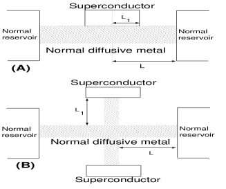
FIG. 1.: The structures considered.

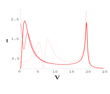
FIG. 2.: The dependence of $t(\epsilon)(2r_{b})^{2}$ on energy, of the structure shown in Fig 1.(B), for different values of the exchange field $h=0$ (solid line) , $h=1$ (thick dotted line) and $h=7$ (light dashed line), With $\gamma=0.1$, $\Delta=20$,$\Gamma=0.3$,$l_{1}=0$.

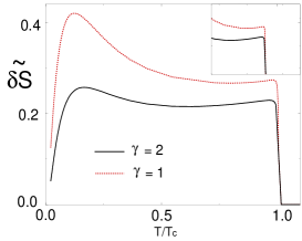
FIG. 3.: Dependence of $\delta\tilde{S}$ on temperature, for the cross geomentry in the weak proximity limit, for different depairing rates $\gamma$. With $\Delta_{0}=20$,$\Gamma=0.1$,$l_{1}=0$. The inset is an enlargement of the second maximum around $T/T_{c}=1.0$. Note the $\delta\tilde{S}=\delta S(2r_{b})^{2}$.

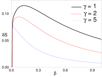
FIG. 4.: Dependence of $\delta S$ on the normalised inverse temperature, for the cross geomentry in the strong proximity limit. For different depairing rates $\gamma$. With $\Delta_{0}=100$,$\Gamma=0.1$,$l_{1}=0$.

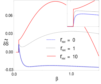
FIG. 5.: Dependence of $\delta\tilde{S}$ on the normalised inverse temperature, for the geomentry shown in Fig. 1A in the weak proximity limit. For different interface resistances $r_{NN^{\prime}}$ . With $\Delta_{0}=10$, $\gamma=0.1$,$\Gamma=0.1$,$l_{1}=0.2$. The inset is an enlargement of the second maximum around $\beta\approx 0.1$. Note $\delta\tilde{S}$ has been scaled for convenience, by 0.1 for $r_{NN^{\prime}}=10$,0.2 for $r_{NN^{\prime}}=1$ and 2 for $r_{NN^{\prime}}=0$.

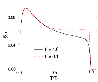
FIG. 6.: Dependence of $\delta\tilde{S}$ on temperature, for the geomentry shown in Fig. 1B in the weak proximity limit. For different damping rates $\Gamma$. With $\Delta_{0}=20$, $\gamma=2$,$\Gamma=0.1$,$l_{1}=0$.

REFERENCES

- [1] C.W.J.Beenakker, Rev.Mod.Phys. 69, 731 (1997).
- [2] C.J. Lambert and R.Raimondi, J. Phys. Cond. Matter 10,5,901 (1998).
- [3] S.N. Artemenko,A.F. Volkov and A.V. Zaitsev, Solid State Comm. 30,771 (1979)
- [4] Yu.V. Nazarov and T.H. Stoof, Phys. Rev. Lett. 76,823 (1996); Phys. Rev. B 53,14496 (1996)
- [5] A.A.Golubov, F.Wilhelm, and A.D.Zaikin, Phys.Rev. B55, 1123 (1996).
- [6] A.F. Volkov and V.V. Pavlovskii, in Correlated Fermions and Transport in Mesoscopic Systems, ed by T. Martin, G. Montambaux and J. Tran Thanh Van, Frontiers, Gif-sur-Yvette Cedex,France,1996
- [7] S.Yip, Phys. Rev. B52, 15504(1995)
- [8] A.F. Volkov, N. Allsopp, and C.J. Lambert, J. Phys. Cond. Matter 8, 45(1996).
- [9] V. N. Gubankov and N. M. Margolin, JETP Letters 29, 673 (1979)
- [10] (a) H. Courtois, Ph. Grandit, D. Mailly, and B. Pannetier, Phys. Rev. Lett. 76, 130 (1996); (b) D. Charlat, H. Courtais, Ph. Grandit, D. Mailly, A.F. Volkov, and B. Pannetier, Phys. Rev. Lett. 77, 4950 (1996).
- [11] S.G.Hartog et al., Phys. Rev. B56, 13738 (1997).
- [12] V.T. Petrashov, R. Sh. Shaikadarov, P. Delsing, and T. Claeson, Pis’ma v ZhETF 67, 489 (1998)
- [13] D. Esteve, H. Pothier, S. Gueron, Norman O. Birge and M.Devoret in Correlated Fermions and Transport in Mesoscopic Systems, ed by T. Martin, G. Montambaux and J. Tran Thanh Van, Frontiers, Gif-sur-Yvette Cedex,France,1996
- [14] A.F.Volkov, K.E.Nagaev,and R.Seviour, Phys.Rev. B57, 5450 (1998)
- [15] A.I. Larkin and Yu.N. Ovchinnikov, in Nonequilibrium Superconductivity, ed. by D.N. Langenberg and A.I. Larkin (Elsevier, Amsterdam, 1986), p.493.
- [16] A.V.Zaitsev, Sov. Phys JETP Lett. 51, 41 (1990); Physica C185-189, 2539(1991).
- [17] A.F.Volkov, A.V.Zaitsev, and T.M.Klapwijk, Physica C210, 21 (1993).
- [18] A.F.Volkov and T.M.Klapwijk, Phys.Lett. A168, 217 (1992).
- [19] F. Zhou, B.Z. Spivak, and A. Zyuzin, Phys. Rev. B52, 4467(1995).
- [20] A.F. Volkov and A.V. Zaitsev, Phys. Rev. B53, 9267(1996).
- [21] C.-J.Chien and V.Chandrasekhar, cond-mat/9805298
- [22] R. Seviour, C.J. Lambert and A.F. Volkov, Phys. Rev. B58, issue 17 (1 Nov 1998)
- [23] A.A. Abrikosov, Fundamentals of the Theory of metals, North-Holland Amsterdam (1988)