The Elasticity of an Electron Liquid

Abstract

The zero temperature response of an interacting electron liquid to a time-dependent vector potential of wave vector $q$ and frequency $\omega$ such that $q\ll q_{F}$, $qv_{F}\ll\omega\ll E_{F}/\hbar$ (where $q_{F}$, $v_{F}$ and $E_{F}$ are the Fermi wavevector, velocity and energy respectively) is equivalent to that of a continuous elastic medium with nonvanishing shear modulus $\mu$, bulk modulus $K$, and viscosity coefficients $\eta$ and $\zeta$. We establish the relationship between the visco-elastic coefficients and the long-wavelength limit of the “dynamical local field factors” $G_{L(T)}(q,\omega)$, which are widely used to describe exchange-correlation effects in electron liquids. We present several exact results for $\mu$, including its expression in terms of Landau parameters, and practical approximate formulas for $\mu$, $\eta$ and $\zeta$ as functions of density. These are used to discuss the possibility of a transverse collective mode in the electron liquid at sufficiently low density. Finally, we consider impurity scattering and/or quasiparticle collisions at non zero temperature. Treating these effects in the relaxation time ($\tau$) approximation, explicit expressions are derived for $\mu$ and $\eta$ as functions of frequency. These formulas exhibit a crossover from the collisional regime ($\omega\tau\ll 1$), where $\mu\sim 0$ and $\eta\sim nE_{F}\tau$, to the collisionless regime ($\omega\tau\gg 1$), where $\mu\sim nE_{F}$ and $\eta\sim 0$.

]

I Introduction

The response of a solid body to external macroscopic forces is described by the theory of elasticity.[1] In a homogeneous and isotropic body [2] the response is controlled by two real elastic constants, the bulk modulus $K$ and the shear modulus $\mu$: dissipation is negligible.

The macroscopic response of a liquid system, on the other hand, is usually described in terms of the Navier-Stokes equation [3] of classical hydrodynamics. This is, at first sight, very different from elasticity. First of all, by the very definition of liquid, the shear modulus vanishes. Second, there is dissipation, due to the two viscosity coefficients $\eta$ and $\zeta$ – the “shear” and “bulk” viscosities respectively. Only the bulk modulus remains approximately the same in the liquid as in the solid state.

Such a sharp distinction disappears at finite frequencies, where liquids develop solid-like characteristic, namely, a non vanishing shear modulus. Both liquids and solids follow a common visco-elastic behavior, which can be mathematically described by a single set of equations (say the equations of elasticity) with complex frequency-dependent elastic constants

$$\tilde{K}(\omega)=K(\omega)-i\omega\zeta(\omega)\,,$$ (1)

and

$$\tilde{\mu}(\omega)=\mu(\omega)-i\omega\eta(\omega)\,.$$ (2)

The visco-elastic coefficients $K$, $\mu$, $\zeta$, $\eta$ on the right hand side are all real functions of frequency.

The crucial parameter that controls the prevalence of solid-like or liquid-like behavior in the liquid is $\omega\tau$, the ratio of the frequency to the inverse of the relaxation time $\tau$ – the time it takes the system to return to thermal equilibrium after being slightly disturbed from it. If $\omega\tau\ll 1$ one is in the collision-dominated (or hydrodynamic) regime, in which $\mu(\omega)$ is negligible and $\eta(\omega)$, $\zeta(\omega)$ are finite. If, on the other hand, $\omega\tau\gg 1$ one is in the collisionless (or elastic) regime, where $\mu(\omega)$ has a finite value, while the viscosities are small. In either case, the bulk modulus does not show a significant dependence on frequency.

In this paper we explore the possibility of describing the long wavelength dynamics of a quantum Fermi liquid [4] near the absolute zero of temperature in terms of classical visco-elastic equations of motion. Limiting ourselves to the linear response of the quantum liquid to an external vector potential $\vec{A}(q,\omega)$ of wave vector $q$ and frequency $\omega$ we shall show that the visco-elastic description is possible (and useful) in the regime

$$q\ll q_{F},~{}~{}~{}~{}~{}q\ll\omega/v_{F},$$ (3)

where $v_{F}$ is the quasiparticle Fermi velocity and $q_{F}$ is the Fermi wave vector. In other words, the frequency must be high compared to the characteristic energy of quasiparticle-quasihole pairs at wave vector $q$, which tends to zero when $q\to 0$ (see Figure 1).

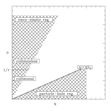
FIG. 1.: The region below the line $\omega=v_{F}q$ is the quasiparticle-quasihole regime. The viscoelastic approach applies to the region $\omega\gg v_{F}q$. The line $\omega=1/\tau$ separates the collisional viscoelastic regime and the collisionless viscoelastic one.

The viscoelastic coefficients will be expressed in terms of the long wavelength limit of the dynamical local field factors $G_{L(T)}(q,\omega)$: these are mathematical constructs (defined below) that are widely used to describe exchange-correlation effects in Fermi liquids.

Most of this paper is devoted to the task of calculating the viscoelastic coefficients of an electron liquid (both in three and two dimensions) in the limit of $\omega\to 0$, that is, in practice, for $\omega\ll E_{F}$ but still satisfying the condition (3). Such coefficients are particularly relevant in the framework of Time-Dependent Density Functional Theory,[5] where they fully determine the low-frequency regime.

We first consider the case of a uniform (translationally invariant) electron gas at the absolute zero of temperature. In this case the low-frequency elastic constants $K$ and $\mu$ can be expressed exactly in terms of the Landau parameters $F_{0}$, $F_{1}$ and $F_{2}$ – at least insofar as the Landau theory of Fermi liquids applies. The result for the bulk modulus [$K=n^{2}d^{2}\epsilon(n)/dn^{2}$, where $\epsilon(n)$ is the ground-state energy density and $n$ is the particle density] has been known for a long time [4, 6] and can be straightforwardly evaluated from the knowledge of the ground state energy. [7, 8] The result for the shear modulus is (to the best of our knowledge) new and, unfortunately, not so easy to evaluate. For this reason, we propose an approach “à la Wigner”, namely we calculate the shear modulus at both high and low densities – where the calculation can be done with relative ease – and interpolate between these two limits. The proposed interpolation function is close to the results of recent mode-coupling calculations of the dynamical local field factor[9] at sufficiently high density.

We proceed in a similar way to the calculation of the viscosities. First the shear viscosity $\eta$ is analytically calculated in the high density limit, making use the formalism of Nifosí et al.,[9] for the imaginary part of the dynamical local field factor. Then we devise a numerical fit that reduces to the analytical result in the high density limit and reproduces the numerical data of Nifosí et al.,[9] at lower density. The bulk viscosity $\zeta$ is found to be approximately zero in this approach.

The last part of the paper is devoted to the treatment of relaxation effects caused either by collisions with impurities or by collisions between thermally excited quasiparticles. We assume that both effects can be described by a single relaxation time $\tau$, such that $1/\tau\ll E_{F}$, and make use of the standard “relaxation time approximation” (RTA) [10] to approximate the collision integral in the quasiparticle transport equation. The low-frequency regime now splits into two distinct regimes: collisional ($\omega\tau\ll 1$) and collisionless ($\omega\tau\gg 1$). The restriction given by Eq. (3) remains in force in both regimes. By solving the transport equation in the RTA we obtain explicit expressions for the elastic and viscous coefficients. In the collisionless regime, these expressions reduce to the ones derived in the first part of the paper. In the collisional regime, they are very different: the shear modulus vanishes (as expected for an ordinary liquid), and the shear viscosity tends to the limit $\eta=\mu\tau$ where $\mu$ is the collisionless shear modulus. Our simple analytic expressions clearly exhibit the crossover from the collisional to the collisionless regime.[11]

We have emphasized the importance of the condition  (3) that assures the possibility of a visco-elastic description of the dynamics of the Fermi liquid. What happens if this condition is violated? The behavior of the microscopic current-current response function of a Fermi liquid changes dramatically as one goes from the $q\ll\omega/v_{F}$ regime to the $q\gg\omega/v_{F}$ regime, even though $q$ and $\omega$ remain small compared to $q_{F}$ and $E_{F}$ respectively. The physical reason is that the response in the second region is dominated by electron-hole excitations that are absent in the first. Because of the change in the character of the response, the current does not obey classical visco-elastic equations of motion in the second regime. Alternatively, if one insisted on casting the equation for the current in a visco-elastic form, one would be forced to use visco-elastic coefficients that diverge in the $q\to 0$ limit. This shows that the visco-elastic theory is not a natural description of the physics for $\omega<qv_{F}$.

This paper is organized as follows:

In Section II we briefly review elasticity, hydrodynamics, and the local field factor representation of the current-current response functions of a Fermi liquid. We establish the relationship between the dynamical local field factors and the frequency-dependent visco-elastic coefficients of Eqs. (1-2).

In Section III we derive an exact expression for the shear modulus of the Fermi liquid at $T=0$ in term of Landau parameters, and a rigorous upper bound on the value of the elastic constants.

In Section IV we present approximate analytical expressions for the evaluation of the visco-elastic coefficients of an interacting electron liquid as functions of density. These expressions are used to discuss the possibility of a transverse sound mode in the low density electron gas.

In Section V we include electron-impurity and thermally induced quasiparticle collisions via Mermin’s relaxation time approximation. We provide explicit formulas for the frequency dependent (on the scale of the inverse relaxation time) shear modulus and viscosity, exhibiting the crossover between the collisional and the collisionless regimes.

II Viscoelastic constants of a Fermi liquid

A Macroscopic equations

The equation of motion for the elastic displacement field $\vec{u}(\vec{r},t)$ in a homogeneous and isotropic solid is [1]

$$mn{\partial^{2}\vec{u}\over\partial t^{2}}=\left[K+\left(1-{2\over d}\right)\mu\right]\vec{\nabla}(\vec{\nabla}\cdot\vec{u})+\mu\nabla^{2}\vec{u}+\vec{F}(\vec{r},t)$$ (4)

where $K$ and $\mu$ are constants, known as the bulk and the shear modulus respectively, $d$ is the number of space dimensions, $\vec{F}(\vec{r},t)$ is an externally applied volume force density, $n$ is the equilibrium number density, and $m$ is the mass of the particles.

We consider periodic forces of the form

$$\vec{F}(\vec{r},t)=\vec{F}(\vec{q},\omega)e^{i(\vec{q}\cdot\vec{r}-\omega t)}+c.c.,$$ (5)

which induce periodic displacements

$$\vec{u}(\vec{r},t)=\vec{u}(\vec{q},\omega)e^{i(\vec{q}\cdot\vec{r}-\omega t)}+c.c.$$ (6)

In order to make contact, later, with microscopic theories of Fermi liquids, we write the force as the time derivative of a vector potential [12]

$$\vec{F}(\vec{r},t)=n{\partial\vec{A}(\vec{r},t)\over\partial t}$$ (7)

and introduce the current density

$$\vec{j}(\vec{r},t)=n{\partial\vec{u}(\vec{r},t)\over\partial t}$$ (8)

as its conjugate field. The equation of motion (4), written in terms of the Fourier transform of the current density, takes the form

$$-i\omega m\vec{j}(\vec{q},\omega) = \left[{K\over n}+\left(1-{2\over d}\right){\mu\over n}\right]{\vec{q}[\vec{q}\cdot\vec{j}(\vec{q},\omega)]\over i\omega}$$ (10)

$$+{\mu\over n}{q^{2}\over i\omega}\vec{j}(\vec{q},\omega)-i\omega n\vec{A}(\vec{q},\omega).$$

Both the current and the vector potential can be written as sums of longitudinal and transverse components (parallel and perpendicular to $\vec{q}$ respectively) $\vec{j}=\vec{j}_{L}+\vec{j}_{T}$, $\vec{A}=\vec{A}_{L}+\vec{A}_{T}$ and the equations of motion for longitudinal and transverse components decouple. The solution of Eq. (10) is

$$\vec{j}_{L}(\vec{q},\omega)={n/m\over 1-\left[{K\over n^{2}}+2\left(1-{1\over d}\right){\mu\over n^{2}}\right]{nq^{2}\over m\omega^{2}}}\vec{A}_{L}(\vec{q},\omega)$$ (11)

and

$$\vec{j}_{T}(\vec{q},\omega)={n/m\over 1-{\mu\over n^{2}}{nq^{2}\over m\omega^{2}}}\vec{A}_{T}(\vec{q},\omega).$$ (12)

We note that $\vec{j}_{L}(\vec{q},\omega)$ is related to the induced density change $n_{1}(\vec{q},\omega)$ by the continuity equation

$$n_{1}(\vec{q},\omega)={\vec{q}\over\omega}\cdot\vec{j}_{L}(\vec{q},\omega)$$ (13)

and the longitudinal vector potential $\vec{A}_{L}(\vec{q},\omega)$ is equivalent, modulo a gauge transformation, to a scalar potential $V(\vec{q},\omega)$ such that

$$\vec{A}_{L}(\vec{q},\omega)={\vec{q}\over\omega}V(\vec{q},\omega).$$ (14)

In writing these equations we have assumed that the external field $\vec{A}_{L}$ includes, self-consistently, the contribution of the mean electrostatic field generated by the density fluctuation $n_{1}$ [the Hartree field $V_{H}=v(q)n_{1}$].

Let us now consider the classical hydrodynamical equation for the current density in a liquid.[3] In the linear approximation with respect to $\vec{j}$ and $\vec{A}$ it has the form

$$-i\omega m\vec{j}(\vec{q},\omega) = \left[{K\over n}-{i\omega\zeta\over n}+\left(1-{2\over d}\right){i\omega\eta\over n}\right]{\vec{q}[\vec{q}\cdot\vec{j}(\vec{q},\omega)]\over i\omega}$$ (16)

$$+{i\omega\eta\over n}{q^{2}\over i\omega}\vec{j}_{1}(\vec{q},\omega)-i\omega n\vec{A}(\vec{q},\omega),$$

where we have used the continuity equation  (13) to rewrite the hydrostatic pressure term in the Euler equation[3] as

$$-\vec{\nabla}p(\vec{q},\omega)=-{dp(n)\over dn}\vec{\nabla}n_{1}(\vec{q},\omega)={dp(n)\over dn}\vec{q}\left[{\vec{q}\cdot\vec{j}_{(}\vec{q},\omega)\over i\omega}\right].$$ (17)

The constants $\eta$ and $\zeta$ are the shear and bulk viscosity coefficients respectively; $p(n)$ is the equilibrium pressure as a function of density and is related to the bulk modulus by the relation $K=ndp(n)/dn$.

Equations  (16) and  (10) are very similar. The hydrodynamic equation differs from the elastic equation through the following replacements: (i) The shear modulus $\mu$ is replaced by the imaginary quantity $-i\omega\eta$, which vanishes at $\omega=0$ in agreement with the notion that a liquid has no resistance to shear. (ii) The bulk modulus $K$ acquires an imaginary part $-i\omega\zeta$ where $\zeta$ is the bulk viscosity.

These observations suggest the use of a single language - say that of elasticity theory - to describe both the liquid and the solid. In this generalized scheme, the equation of motion becomes

$$-i\omega m\vec{j}(\vec{q},\omega) = \left[{\tilde{K}(\omega)\over n}+\left(1-{2\over d}\right){\tilde{\mu}(\omega)\over n}\right]{\vec{q}[\vec{q}\cdot\vec{j}(\vec{q},\omega)]\over i\omega}$$ (19)

$$+{\tilde{\mu}(\omega)\over n}{q^{2}\over i\omega}\vec{j}(\vec{q},\omega)-i\omega n\vec{A}(\vec{q},\omega),$$

where $\tilde{\mu}(\omega)$ and $\tilde{K}(\omega)$ are the frequency-dependent visco-elastic constants defined in the introduction [Eqs. (1-2)].

The solution of this equation of motion is

$$\vec{j}_{L}(\vec{q},\omega)={n/m\over 1-\left[{\tilde{K}(\omega)\over n^{2}}+2\left(1-{1\over d}\right){\tilde{\mu}(\omega)\over n^{2}}\right]{nq^{2}\over m\omega^{2}}}\vec{A}_{L}(\vec{q},\omega)$$ (20)

and

$$\vec{j}_{T}(\vec{q},\omega)={n/m\over 1-{\tilde{\mu}(\omega)\over n^{2}}{nq^{2}\over m\omega^{2}}}\vec{A}_{T}(\vec{q},\omega).$$ (21)

The key difference between a solid and a liquid is that the solid has an essentially real $\tilde{\mu}$ ($\mu$ finite, $\eta\sim 0$), whereas a liquid has an essentially imaginary $\tilde{\mu}$ ($\eta$ finite, $\mu\sim 0$). As for the generalized bulk modulus, its real part (related to the compressibility) is nearly the same in the two phases. The bulk viscosity is generally of the same order of magnitude as the shear viscosity,[3] but, in the case of the electron liquid, it will be shown to vanish within the mode-coupling approximation of Ref. [9].

B Connection with microscopic linear response theory

Let us now turn to the microscopic formulation of the linear response of a homogeneous, isotropic body, subjected to an external vector potential $\vec{A}(\vec{q},\omega)$. The proper response functions $\chi_{L}(\vec{q},\omega)$ and $\chi_{T}(\vec{q},\omega)$ (longitudinal and transverse respectively) are defined by the relations

$$\vec{j}_{L(T)}(\vec{q},\omega)=\chi_{L(T)}(\vec{q},\omega)\vec{A}_{L(T)}(\vec{q},\omega).$$ (22)

A useful way of representing $\chi_{L(T)}$ is [13]

$$\chi_{L(T)}(\vec{q},\omega)={\chi^{0}_{L(T)}(\vec{q},\omega)\over 1+v(q)G_{L(T)}(\vec{q},\omega)(q^{2}/\omega^{2})\chi^{0}_{L(T)}(\vec{q},\omega)},$$ (23)

where

$$\chi^{0}_{L(T)}(\vec{q},\omega)={n\over m}+\sum_{\vec{k}}\left({k_{L(T)}\over m}\right)^{2}{f(\epsilon_{k+q})-f(\epsilon_{k})\over\omega+\epsilon_{k+q}-\epsilon_{k}}$$ (24)

are the longitudinal (transverse) response functions of the noninteracting electron gas, $\epsilon_{k}=k^{2}/2m$ is the free particle energy, $f(\epsilon_{k})$ is the Fermi distribution function, and $k_{L(T)}$ is the longitudinal (transverse) component of $\vec{k}$ relative to $\vec{q}$, and $v(q)$ is the Fourier transform of the interaction [$v(q)=4\pi e^{2}/q^{2}$ and $v(q)=2\pi e^{2}/q$ in three and two dimensions respectively]. The dynamical local field factors $G_{L(T)}(\vec{q},\omega)$ are effectively defined by these equations: they take into account exchange-correlation effects beyond the random phase approximation.

Note that, with these definitions, the longitudinal local field factor $G_{L}$ coincides with the more familiar scalar local field factor $G$ used in the theory of the density-density response function in Ref. [13] for example.

Let us now consider the long wavelength limit ($qv_{F}\ll\omega$) of $\chi_{L(T)}(q,\omega)$. Expanding the noninteracting response functions  (24) we find

$$\chi_{L(T)}(\vec{q},\omega) \simeq {n\over m}\left[1+\alpha_{L(T)}^{(d)}{E_{F}\over n}{nq^{2}\over m\omega^{2}}\right.$$ (26)

$$\hskip 28.45274pt\left.+f_{xcL(T)}(\omega){nq^{2}\over m\omega^{2}}\right],$$

where

$$f_{xcL(T)}(\omega)\equiv-\lim_{q\to 0}v(q)G_{L(T)}(q,\omega)$$ (27)

are complex functions of frequency, which satisfy Kramers-Krönig dispersion relations between their real and imaginary parts (see discussion in the next section) and $\alpha_{L}^{(3)}=6/5$, $\alpha_{L}^{(2)}=3/2$, $\alpha_{T}^{(3)}=2/5$, $\alpha_{T}^{(2)}=1/2$.

Comparing Eq. (26) with the macroscopic response functions  (20) and  (21) we are led to the following identifications:

$$\tilde{\mu}(\omega)=\alpha_{T}^{(d)}nE_{F}+n^{2}f_{xcT}(\omega)$$ (28)

and

$$\tilde{K}(\omega) = \left[\alpha_{L}^{(d)}-\left(2-{2\over d}\right)\alpha_{T}^{(d)}\right]nE_{F}$$ (30)

$$+n^{2}\left[f_{xcL}(\omega)-\left(2-{2\over d}\right)f_{xcT}(\omega)\right]\,.$$

Separating the real and imaginary parts of these equations, and taking the limit $\omega\to 0$ (but still with $\omega\gg qv_{F}$), we arrive at the promised expressions for the elastic and viscosity coefficients in terms of the long wavelength limit of the local field factors:

$$\mu=\alpha_{T}^{(d)}nE_{F}+n^{2}{\bf Re}f_{xcT}(0),$$ (31)

$$K = \left[\alpha_{L}^{(d)}-\left(2-{2\over d}\right)\alpha_{T}^{(d)}\right]nE_{F}$$ (33)

$$+n^{2}{\bf Re}\left[f_{xcL}(0)-\left(2-{2\over d}\right)f_{xcT}(0)\right],$$

$$\eta=-n^{2}\lim_{\omega\to 0}{{\bf Im}f_{xcT}(\omega)\over\omega},$$ (34)

$$\zeta=-n^{2}\lim_{\omega\to 0}\left({{\bf Im}f_{xcL}(\omega)\over\omega}-\left(2-{2\over d}\right){{\bf{Im}}f_{xcT}(\omega)\over\omega}\right]$$ (35)

Equations  (31–35) are the main result of this Section. We underline the fact that they have been obtained under the assumption $qv_{F}\ll\omega$. Outside this regime, e.g., for $\omega<qv_{F}$, the microscopic response functions do not yield visco-elastic equations of motion or, equivalently, the visco-elastic coefficients diverge for $q\to 0$. The analysis of this non-viscoelastic regime is beyond the scope of this paper.

III The calculation of the elastic constants: rigorous results

A Expression in terms of Landau parameters

The elastic constants of a Fermi liquid can be exactly expressed in terms of Landau parameters, insofar as the Landau theory of Fermi liquids is valid. To see this, we begin by deriving the equation of motion for the quasiparticle distribution function in the presence of a slowly varying vector potential $\vec{A}(\vec{r},t)$.

Following the discussion of Nozières and Pines [4] we treat the quasiparticles as a gas of non-interacting classical particles governed by a self-consistent Hamiltonian

$$H_{qp}(\vec{r},\vec{p}) = \epsilon_{\vec{p}+\vec{A}(\vec{r},t)}+\sum_{{\vec{p}^{\prime}}}f_{pp^{\prime}}\delta n_{p^{\prime}}(\vec{r},t)$$ (36)

$$\simeq \epsilon(\vec{p})+{\vec{p}\cdot\vec{A}(\vec{r},t)\over m^{*}}+\sum_{\vec{p}^{\prime}}f_{pp^{\prime}}\delta n_{p^{\prime}}(\vec{r},t),$$ (37)

where $\epsilon_{\vec{p}}$ is the quasiparticle energy, $\vec{\nabla}_{p}\epsilon_{\vec{p}}\equiv\vec{v}_{p}=\vec{p}/m^{*}$ is the quasiparticle velocity, $m^{*}$ is the effective mass, and $f_{pp^{\prime}}$ are Landau parameters. This approach is justified in the limit of zero temperature and zero frequency, since the excited quasiparticles have an essentially infinite lifetime in this regime, and their mutual collisions are negligible.

The self-consistent nature of the quasiparticle Hamiltonian is apparent in the last term, which is proportional to the departure of the quasiparticle phase space distribution function $n_{p}(\vec{r},t)$ from the local equilibrium distribution $n_{0}(\epsilon_{\vec{p}+\vec{A}})$:

$$\delta n_{p}(\vec{r},t) = n_{p}(\vec{r},t)-n_{0}(\epsilon_{\vec{p}+\vec{A}})$$ (38)

$$\simeq n_{p}(\vec{r},t)-n_{0}(\epsilon_{p})-n_{0}^{\prime}(\epsilon_{p}){\vec{p}\cdot\vec{A}(\vec{r},t)\over m^{*}}$$ (39)

$$= n_{1p}-n_{0}^{\prime}(\epsilon_{p}){\vec{p}\cdot\vec{A}(\vec{r},t)\over m^{*}}.$$ (40)

Here $n_{0}(\epsilon_{p})=\theta(\epsilon_{p_{F}}-\epsilon_{p})$ is the true equilibrium distribution function at $T=0$ and chemical potential $\epsilon_{p_{F}}$, $n_{0}^{\prime}(\epsilon_{p})=-\delta(\epsilon_{p_{F}}-\epsilon_{p})$ is its derivative with respect to energy, and

$$n_{1p}(\vec{r},t)=n_{p}(\vec{r},t)-n_{0}(\epsilon_{p})$$ (41)

is the departure of the distribution function from true equilibrium.

The fact that the departure from local rather than true equilibrium appears in Eq. (36) is essential to guarantee particle conservation and gauge invariance of the theory.

We now make use of the well-known Landau relation [4] between bare and effective mass in a translationally invariant system

$${\vec{p}\over m}={\vec{p}\over m^{*}}-\sum_{\vec{p}^{\prime}}f_{pp^{\prime}}n_{0}^{\prime}(\epsilon_{p}^{\prime}){\vec{p}^{\prime}\over m^{*}},$$ (42)

and rewrite the effective Hamiltonian in terms of the departure from true equilibrium [see Eq. (38)]:

$$H_{qp}(\vec{r},\vec{p})=\epsilon(\vec{p})+{\vec{p}\cdot\vec{A}(\vec{r},t)\over m}+\sum_{\vec{p}^{\prime}}f_{pp^{\prime}}n_{1p^{\prime}}(\vec{r},t).$$ (43)

Finally, we write the classical (linearized) Liouville equation for the evolution of the quasiparticle distribution function under $H_{qp}$. After introducing the Fourier representation

$$n_{1p}(\vec{r},t)=n_{1p}(\vec{q},\omega)e^{i(\vec{q}\cdot\vec{r}-\omega t)}+c.c$$ (44)

we obtain the desired equation of motion

$$(\vec{q}\cdot\vec{v}_{p}-\omega)n_{1p}(\vec{q},\omega)$$ (45)

$$-\vec{q}\cdot\vec{v}_{p}n_{0}^{\prime}(\epsilon_{p})\left[\sum_{p^{\prime}}f_{pp^{\prime}}n_{1p^{\prime}}(\vec{q},\omega)+{\vec{p}\over m}\cdot\vec{A}(\vec{q},\omega)\right]=0.$$ (46)

The current response is obtained from the quasiparticle distribution function via the relation

$$\vec{j}(\vec{q},\omega)=\sum_{p}{\vec{p}\over m}n_{1p}(\vec{q},\omega)+{n\over m}\vec{A}_{1}(\vec{q},\omega),$$ (47)

where it must be noted that the bare mass, rather than the effective mass, enters the definition of the current.[4] The density response is given by $n_{1}({\vec{q}},\omega)=\sum_{p}n_{1p}({\vec{q}},\omega)$.

Equation (45) can be solved for a given value of the ratio $x\equiv qv_{F}/\omega$, with both $q$ and $\omega$ tending to zero. After setting

$$n_{1p}({\vec{q}},\omega)=\vec{\Pi}_{\vec{p}}(x)\cdot\vec{A}({\vec{q}},\omega),$$ (48)

we see that $\vec{\Pi}_{\vec{p}}(x)$ obeys the equation of motion

$$\vec{\Pi}_{\vec{p}}(x)=R_{\vec{p}}(x)\left({{\vec{p}}\over m}+\sum_{\vec{p}^{\prime}}f_{{\vec{p}}{\vec{p}^{\prime}}}\vec{\Pi}_{\vec{p}^{\prime}}(x)\right)$$ (49)

where

$$R_{\vec{p}}(x)\equiv n_{0}^{\prime}(\epsilon_{p}){x\cos(\theta)\over x\cos(\theta)-1},$$ (50)

and $\theta$ is the angle between ${\vec{p}}$ and ${\vec{q}}$.

In the $x\to 0$ limit [see Eq. (3)] we expand $R_{\vec{p}}(x)$ and $\vec{\Pi}_{\vec{p}}(x)$ in a power series of $x$ as follows

$$R_{\vec{p}}(x)=-n_{0}^{\prime}(\epsilon_{p})\sum_{n=1}^{\infty}(x\cos{\theta})^{n}$$ (51)

and

$$\vec{\Pi}_{\vec{p}}(x)=\sum_{n=0}^{\infty}\vec{\Pi}_{\vec{p}}^{(n)}x^{n}.$$ (52)

Inserting these expansions in Eq. (49) we obtain the recursion relation

$$\vec{\Pi}_{\vec{p}}^{(n)} = -n_{0}^{\prime}(\epsilon_{p}){\vec{p}\over m}(\cos{\theta})^{n}$$ (54)

$$-n_{0}^{\prime}(\epsilon_{p})\sum_{\vec{p}^{\prime}}f_{{\vec{p}}{\vec{p}^{\prime}}}\sum_{m=0}^{n-1}\vec{\Pi}_{\vec{p}^{\prime}}^{(m)}(\cos{\theta})^{n-m},$$

with $\vec{\Pi}_{\vec{p}}^{(0)}=0$ and $\vec{\Pi}_{\vec{p}}^{(1)}=-n_{0}^{\prime}(\epsilon_{p})\vec{p}\cos{\theta}/m$. The relevant term is the one with $n=2$:

$$\vec{\Pi}_{\vec{p}}^{(2)} = -n_{0}^{\prime}(\epsilon_{p})\left[{\vec{p}\over m}(\cos{\theta})^{2}\right.$$ (56)

$$\left.-\sum_{\vec{p}^{\prime}}f_{{\vec{p}}{\vec{p}^{\prime}}}\cos{\theta}n_{0}^{\prime}(\epsilon_{p^{\prime}}){{\vec{p}^{\prime}}\over m}\cos{\theta^{\prime}}\right].$$

This enables us to calculate the current, and hence the response function, exactly to order $x^{2}=(qv_{F}/\omega)^{2}$. More precisely, making use of Eq. (47) we obtain (from now on, we focus on 3D)

$$\chi_{L}-{n\over m} = \sum_{\vec{p}}{\hat{q}\cdot{\vec{p}}\over m}\hat{q}\cdot\vec{\Pi}_{\vec{p}}^{(2)}(x)x^{2}$$ (57)

$$= {nq^{2}\over m\omega^{2}}{q_{F}^{2}\over m^{2}}{3/5+4F_{2}/75+F_{0}/3\over 1+F_{1}/3}$$ (58)

and

$$\chi_{L}+2\chi_{T}-3{n\over m} = \sum_{\vec{p}}{{\vec{p}}\over m}\cdot\vec{\Pi}_{\vec{p}}(x)x^{2}$$ (59)

$$= {nq^{2}\over m\omega^{2}}{q_{F}^{2}\over m^{2}}{1+2F_{2}/15+F_{0}/3\over 1+F_{1}/3},$$ (60)

where $F_{l}$ are the usual dimensionless Landau parameters.[4] The following partial results have been used to evaluate the sums over ${\vec{p}}$ and ${\vec{p}^{\prime}}$ in three dimensions

$$\sum_{{\vec{p}}{\vec{p}^{\prime}}}n_{0}^{\prime}(\epsilon_{p})n_{0}^{\prime}(\epsilon_{p^{\prime}})f_{{\vec{p}}{\vec{p}^{\prime}}}(\hat{q}\cdot{\vec{p}})^{2}(\hat{q}\cdot{\vec{p}^{\prime}})^{2}=$$ (61)

$${q_{F}^{4}N(0)\over 9}\left(F_{0}+{4\over 25}F_{2}\right)$$ (62)

and

$$\sum_{{\vec{p}}{\vec{p}^{\prime}}}n_{0}^{\prime}(\epsilon_{p})n_{0}^{\prime}(\epsilon_{p^{\prime}})f_{{\vec{p}}{\vec{p}^{\prime}}}(\hat{q}\cdot{\vec{p}})(\hat{q}\cdot{\vec{p}^{\prime}})({\vec{p}}\cdot{\vec{p}^{\prime}})=$$ (63)

$${q_{F}^{4}N(0)\over 9}\left(F_{0}+{2\over 5}F_{2}\right)$$ (64)

where $N(0)=m^{*}q_{F}/\pi^{2}$ is the three-dimensional density of quasiparticle states at the Fermi surface.

A direct comparison between Eqs. (57, 59) and Eq. (26) yields the desired expressions for $f_{xcL(T)}(0)$:

$${\bf{Re}}f_{xcL}(0)={6E_{F}\over 5n}{{5\over 9}F_{0}+{4\over 45}F_{2}-{1\over 3}F_{1}\over 1+{1\over 3}F_{1}}$$ (65)

and

$${\bf{Re}}f_{xcT}(0)={2E_{F}\over 5n}{{1\over 5}F_{2}-{1\over 3}F_{1}\over 1+{1\over 3}F_{1}}$$ (66)

Similar results are obtained in two dimensions:

$${\bf{Re}}f_{xcL}(0)={2E_{F}\over n}{{1\over 2}F_{0}-{3\over 8}F_{1}+{1\over 8}F_{2}\over 1+{1\over 2}F_{1}}\,,$$ (67)

$${\bf{Re}}f_{xcT}(0)={2E_{F}\over n}{{1\over 8}F_{2}-{1\over 8}F_{1}\over 1+{1\over 2}F_{1}}$$ (68)

Substituting in Eqs. (31) and (33) we obtain the following expressions for the elastic constants. In three dimensions

$$K=n^{2}{d^{2}\epsilon(n)\over dn^{2}}={2nE_{F}\over 3}{1+F_{0}\over 1+{1\over 3}F_{1}}$$ (69)

and

$$\mu={2nE_{F}\over 5}{1+F_{2}/5\over 1+F_{1}/3}.$$ (70)

In two dimensions

$$K={nE_{F}}{1+F_{0}\over 1+{1\over 2}F_{1}}\,.$$ (71)

and

$$\mu={nE_{F}\over 2}{1+F_{2}/2\over 1+F_{1}/2}.$$ (72)

These are the main results of this Section. There is no surprise as far as the bulk modulus is concerned: it is given by the standard thermodynamic expression, where the energy density can be calculated by Quantum Monte Carlo. The shear modulus, on the other hand, has an expression involving Landau parameters, which are not easily calculated from Monte Carlo simulations, even though some progress in this direction has recently been reported.[14]

B Rigorous upper bounds on the elastic constants

In this Section we derive two exact bounds on the elastic constants, which follow from the Kramers-Kronig dispersion relations between the real and the imaginary parts of $f_{xcL(T)}(\omega)$. The origin of these relations can be easily seen from the formula

$$f_{xcL(T)}(\omega)=\lim_{q\to 0}{\omega^{2}\over q^{2}}\left([\chi^{(0)}_{L(T)}]^{-1}(q,\omega)-\chi_{L(T)}^{-1}(q,\omega)\right)$$ (73)

which directly follows from the representation  (23) and the definition  (27). Both $\chi$ and $\chi^{(0)}$ are analytic functions of frequency in the upper half plane of this variable, and both have no zeroes in this domain.[15] This implies that their inverses are also analytic everywhere in the upper half plane. The large frequency behavior of Eq. (73) is regular because $\chi$ and $\chi^{(0)}$ have the same form [$n/m+O(q^{2}/\omega^{2}$)] in this limit. From this, one can also see that the $q\to 0$ limit is well behaved.

From these considerations we conclude that the Kramers-Krönig relations must hold in the standard form

$${\bf{Re}}f_{xcL(T)}(\omega) = {\bf{Re}}f_{xcL(T)}(\infty)$$ (75)

$$+{2\over\pi}{\cal P}\int_{0}^{\infty}d\omega^{\prime}{\omega^{\prime}{\bf{Im}}f_{xcL(T)}(\omega^{\prime})\over(\omega^{\prime})^{2}-\omega^{2}}$$

where ${\cal P}$ denotes the Cauchy principal part. The second law of thermodynamics (positivity of dissipation) requires that ${\bf Im}\chi_{L(T)}(q,\omega)\leq 0$ at all positive frequencies. But ${\bf Im}\chi^{(0)}_{L(T)}(q,\omega)=0$ for $qv_{F}\ll\omega$ [see Eq. (24)]. Thus, from Eq. (73), we see that

$${\bf{Im}}f_{xcL(T)}(\omega)\leq 0$$ (76)

for all positive frequencies. It then follows from Eq. (75) that

$$f_{xcL(T)}(0)\leq f_{xcL(T)}(\infty).$$ (77)

Recall now that the right hand side of Eq. (77) can be expressed exactly, via the first moment of the current-current spectral function, in terms of the expectation values of the kinetic and potential energy in the ground state (a brief derivation is given in Appendix A):

$$f_{xcL}(\infty)={1\over 2n}\left[{12\over d}(\langle ke\rangle-\langle ke\rangle_{0})+{1+3\beta^{(d)}\over d}\langle pe\rangle\right]$$ (78)

and

$$f_{xcT}(\infty)={1\over 2n}\left[{4\over d}(\langle ke\rangle-\langle ke\rangle_{0})+{\beta^{(d)}-1\over d}\langle pe\rangle\right],$$ (79)

where $\langle ke\rangle$, $\langle ke\rangle_{0}$, and $\langle pe\rangle$ are the expectation values of the kinetic energy, the noninteracting kinetic energy and the potential energy per particle respectively, and $\beta^{(2)}=1/2$, $\beta^{(3)}=1/5$. These quantities can be expressed in terms of the exchange-correlation energy per particle $\epsilon_{xc}(n)$ as follows:

$$\langle ke\rangle-\langle ke\rangle_{0}=dn^{1/d+1}\left({\epsilon_{xc}\over n^{1/d}}\right)^{\prime}$$ (80)

and

$$\langle pe\rangle=-dn^{1+2/d}\left({\epsilon_{xc}\over n^{2/d}}\right)^{\prime},$$ (81)

where $d$ is the dimensionality and the prime denotes differentiation of the function in the round brackets with respect to $n$. The function $\epsilon_{xc}(n)$ is given in Refs. [7, 8] for $3$ and $2$ dimensions respectively.

The $\omega\to\infty$ limit of the longitudinal local field factor was first calculated in three-dimensions by Puff.[16] That result is usually referred to as the “third moment sum rule” [13] since it is related to the third moment of the dynamical structure factor – the spectral function of the density-density response function $\chi$. Because of the relation $\chi=q^{2}\chi_{L}/\omega^{2}$ (which follows from gauge-invariance and from the continuity equation) the third moment of the density-density response function coincides with the first moment of the longitudinal current-current response function. The straightforward extensions to two-dimensions and to the transverse case are outlined in Appendix A.

Combining the foregoing results with our expressions for the elastic constants [Eqs. (70-69)] we obtain the rigorous inequalities

$$\mu\leq\alpha_{T}^{(d)}nE_{F}+n^{2}f_{xcT}(\infty)$$ (82)

$$K+\left(2-{2\over d}\right)\mu\leq\alpha_{L}^{(d)}nE_{F}+n^{2}f_{xcL}(\infty),$$ (83)

with the coefficients $\alpha$ defined after Eq. (27). The usefulness of these inequalities arises from the fact that the quantities on the right hand sides are ground-state properties, which can be calculated by Quantum Monte Carlo. Notice that the inequalities are satisfied as strict equalities whenever the dissipation vanishes, i.e., when ${\bf{Im}}f_{xcL(T)}=0$ at all frequencies. In an electron liquid, this happens both in the first order approximation with respect to the strength of the Coulomb interaction (weak coupling regime), and in the strong coupling limit, when the electrons are expected to form a Wigner crystal.[17] This observation leads us to suggest that the right hand side of Eqs. (82) and  (83) may provide good approximation to the elastic constants at all coupling strengths.

IV Approximate expressions for the shear modulus and viscosity of an electron liquid

A High-density limit

In the regime $na_{B}^{d}\gg 1$ where $a_{B}$ is the Bohr radius, the effect of the Coulomb interaction is small, and can be treated by first-order perturbation theory. It is straigthforward to show that the $f_{xcL(T)}(\omega)$’s are real and independent of frequency in this approximation. This is because, in the limit $q\to 0$, the imaginary part of the current-current response functions arises from processes involving at least two electron-hole pair excitations: such processes are not allowed in first-order perturbation theory. The vanishing of ${\bf Im}f_{xcL(T)}(\omega)$, combined with the dispersion relations  (75) implies that ${\bf Re}f_{xcL(T)}(\omega)$ is independent of frequency. Hence Eq. (77) holds as a strict equality. Since $\langle ke\rangle=\langle ke\rangle_{0}={d\over d+2}E_{F}$, $\langle pe\rangle=-(3/4)e^{2}k_{F}/\pi$ for $d=3$ and $\langle pe\rangle=-(4/3)e^{2}k_{F}/\pi$ for $d=2$ in the first order approximation we obtain

$$\mu(n)={2nE_{F}\over 5}+{ne^{2}k_{F}\over 10\pi}$$ (84)

(3 dimensions, $na_{B}^{3}\gg 1$) and

$$\mu(n)={nE_{F}\over 2}+{ne^{2}k_{F}\over 6\pi}$$ (85)

(2 dimensions, $na_{B}^{2}\gg 1$). These results can also be obtained directly from Eqs. (70,72) of Section III A, making use of the first-order expression for the Landau parameters, $f_{{\vec{p}}{\vec{p}^{\prime}}}=-v({\vec{p}}-{\vec{p}^{\prime}})/2$.

Let us now turn to the calculation of the high-density limit of the viscosities $\eta$ and $\zeta$. Our starting point is the second-order expression for ${\bf Im}f_{xcL(T)}(\omega)$, which is obtained from Eq. (11) of Ref. [9] after replacing the response functions $\chi_{L,T}$ by the noninteracting ones $\chi^{0}_{L,T}$ and setting the “exchange correction factor” equal to $1$:

$${\bf Im}f_{xcL(T)}(\omega)=-\int_{0}^{\omega}{d\omega^{\prime}\over\pi}\int{d^{d}q\over(2\pi)^{d}n^{2}}v(q)^{2}$$ (86)

$$\left[a_{L(T)}{q^{2}\over{\omega}^{{}^{\prime}2}}{\bf Im}\chi^{(0)}_{L}(q,\omega^{\prime})+b_{L(T)}{q^{2}\over\omega^{2}}{\bf Im}\chi^{(0)}_{T}(q,\omega^{\prime})\right]$$ (87)

$${q^{2}\over(\omega-\omega^{\prime})^{2}}{\bf Im}\chi^{(0)}_{L}(q,\omega-\omega^{\prime}),$$ (88)

with ($a_{L}$, $a_{T}$, $b_{L}$, $b_{T}$) equal to $(23/30,8/15,8/15,2/5)$ in three dimensions and to $(11/16,9/16,1/2,1/2)$ in two dimensions.

The imaginary parts of the noninteracting response functions $\chi^{(0)}_{L(T)}$ at small $\omega$ and finite $q$ are directly calculated from Eq. (24):

$${q^{2}\over\omega^{2}}{\bf Im}\chi^{(0)}_{L}(q,\omega)\simeq-{d\over 2}{n\over E_{F}}\gamma_{L}{\omega\over qv_{F}}$$ (89)

and

$${\bf Im}\chi^{(0)}_{T}(q,\omega)\simeq-\gamma_{T}{n\over m}{\omega\over qv_{F}},$$ (90)

for $\omega/v_{F}<q<2q_{F}+\omega/v_{F}$; zero otherwise. The constants $(\gamma_{L},\gamma_{T})$ are given by $(\pi/2,3\pi/4)$ for $d=3$ and $(1,2)$ for $d=2$.

From the above formulas, it is easy to see that Eq. (86) gives an infinite result, due to the divergence of the unscreened Coulomb interaction $v(q)$ for $q\to 0$. The result is indeed finite if the screening of the interaction is duly taken into account. In the high-density limit and at low frequency this is accomplished by the use of the Thomas-Fermi statically screened interaction $v(q)\to v^{TF}(q)=4\pi e^{2}/(q^{2}+q_{TF}^{2})$ ($q_{TF}^{2}=6\pi ne^{2}/E_{F}$) in three dimensions, and $v(q)\to v^{TF}(q)=2\pi e^{2}/(q+q_{TF})$ ($q_{TF}=2/a_{B}$) in two dimensions.

The first term in Eq. (86), which involves the product of two $\chi^{(0)}_{L}$’s, is proportional to $\omega^{3}$, and therefore does not contribute to the viscosity coefficients [see Eqs. (34, 35)]. As for the second term, we find, after some tedious but straightforward calculations,

$${\bf Im}f_{xcL(T)}=-\beta_{L(T)}{\omega\over E_{F}^{2}}\int_{0}^{2q_{F}}q^{d-1}[v^{TF}(q)]^{2}dq,$$ (91)

where $\beta_{L(T)}=(3/128\pi)b_{L(T)}$ for $d=3$ and $\beta_{L(T)}=(1/12\pi^{2})b_{L(T)}$ for $d=2$.

Evaluation of the integral and substitution in Eq. (34) leads to our result for the high-density limit of the shear viscosity:

$$\eta\simeq{n\sqrt{\pi}\over 40(a_{B}k_{F})^{3/2}}\simeq{1\over 60}nr_{s}^{3/2}$$ (92)

in three dimensions, and

$$\eta\simeq={r_{s}^{2}\over 6\pi}n\ln{\sqrt{2}\over er_{s}}=0.053r_{s}^{2}n(-\ln r_{s}-0.65)$$ (93)

in two dimensions.

It is interesting to notice that, in the same limit, the bulk viscosity $\zeta$ vanishes, both in three and two dimensions, due to the relationship $b_{L}/b_{T}=2(d-1)/d$.

B Low-density limit

In the regime $na_{B}^{d}\ll 1$ the electron liquid is strongly correlated (via the long-range Coulomb interaction) and its behavior is expected to be similar to that of a classical Wigner crystal. [17] The elastic constants of a classical Wigner crystal have been calculated by various authors.[18, 19] Of particular interest is the case of the hexagonal lattice, which is expected to be the stable crystal structure in two dimensions. [19] The elastic properties of this lattice are formally indistinguishable from those of a homogeneous and isotropic body, i.e. there are only two elastic constants $K$ and $\mu$,[1] and they are given by [19] $\mu\simeq 0.24e^{2}n^{3/2}$ and $K=-6\mu$. (The fact that $K<0$ in an electron liquid should be no cause for alarm because this bulk modulus enters physical properties summed to the Fourier transform of the Coulomb interaction $v(q)$, which is large and positive at long wavelength.) In three dimensions, the Wigner crystal has cubic symmetry, and anisotropic elastic constants. The appropriate low-density limit for the strongly correlated liquid, obtained by averaging over different orientations[20] is $\mu\simeq 0.19e^{2}n^{4/3}$ and $K=-(10/3)\mu$.

Remarkably, we find that in this case, as well as in the weak coupling limit, the inequality (82) is obeyed as a strict equality, namely, substituting on the right hand side of Eq. (82) the potential energy of the Wigner crystal ($\sim-1.8/r_{s}Ryd$ in 3D, $\sim-2.2/r_{s}Ryd$ in 2D), and neglecting the kinetic energy, which tends to zero in the low density limit, one obtains the correct value of $\mu$. This implies that the imaginary parts of $f_{xcL(T)}(\omega)$’s vanish in the low-density limit.

C Interpolation formula

At intermediate densities no exact results for the $f_{xcL(T)}(\omega)$’s are available. A mode-coupling calculation of these quantities for both 2-dimensional and 3-dimensional electron gases has recently been performed by Nifosí et al.[9] Their results are expected to be an improvement upon previous estimates,[21] at least for not too large coupling strengths. Unfortunately, the values of $\mu$ obtained from this approximate theory do not conform to the physical expectation that $\mu$ should reduce to the shear modulus of the classical Wigner crystal in the limit of large $r_{s}$. In fact, the approximate $\mu$ is found to become negative at large $r_{s}$. We believe that this should be regarded as a failure of the approximate theory. For this reason, we propose an interpolation formula for $\mu$ that does not suffer from this problem: it reduces to the correct limits for high and low density, and does not differ substantially from the estimates of Nifosí et al.[9] in the range of $r_{s}$ where the latter are expected to be reliable.

Our approximate formula is

$$\mu/n=ar_{s}^{-2}+br_{s}^{-1}+(c-b){1\over r_{s}+20}$$ (94)

where $a$ and $b$ are obtained from the low-$r_{s}$ limit (in 3D, $a=k_{F}^{2}/5m$ and $b={e^{2}k_{F}/10\pi}$; in 2D, $a=k_{F}^{2}/4m$ and $b=e^{2}k_{F}/6\pi$) and $c$ is obtained from the high-$r_{s}$ limit ($c=0.24Ryd$ in 3D and $c=0.22Ryd$ in 2D). The approximate $\mu(r_{s})$ is plotted in Fig. 2, together with the values of $\mu$ from Ref. [9].

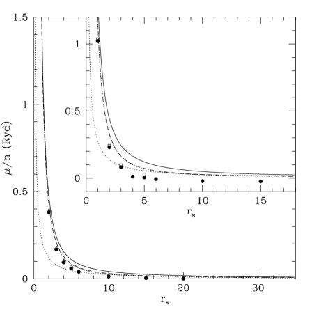
FIG. 2.: Shear modulus $\mu/n$ (full curve) as a function of density in 3D (main figure) and 2D (inset). Dots are from Ref. [9], open squares have been obtained from Eqs. (70-72) using estimates of the Landau parameters from Refs. [14, 22], dotted curves are the asymptotic behaviours of Eqs. (84-85) and from the Wigner crystal (see Section IV B), the full curve is the upper bound of Eq. (82), and the dashed curve is the approximate interpolation of Eq. (94).

An analogous fit can be performed for the shear viscosity $\eta$, with the caveat that in this case the high-$r_{s}$ behaviour is unknown and the advantage that no sign problem is present in the mode-coupling computation. The proposed formulas are

$$\eta\simeq\left(60r_{s}^{-3/2}+c_{1}r_{s}^{-1}+c_{2}r_{s}^{-2/3}+c_{3}r_{s}^{-1/3}\right)^{-1}n$$ (95)

where $c_{1}=80$, $c_{2}=-40$, $c_{3}=62$ in 3 dimensions, and

$$\eta\simeq\left[\left({r_{s}^{2}\over 6\pi}\ln{\sqrt{2}\over er_{s}}+c_{0}r_{s}^{2}\right)^{-1}+c_{1}r_{s}^{-2}+c_{2}r_{s}^{-1/2}+c_{3}\right]^{-1}n$$ (96)

where $c_{0}=0.25$, $c_{1}=21$, $c_{2}=23$, $c_{3}=13$. in 2 dimensions. The resulting functions are compared in Fig. 3 with the values calculated in Ref. [9].

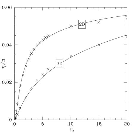
FIG. 3.: Shear viscosity $\eta$ in $d=2$ and $d=3$ (in units of $n$) from the mode-coupling calculation of Nifosì et al.[9] (crosses) compared with the analytical expressions of Eqs. (92-93) (full curves).

D Transverse collective mode in the electron liquid

A transverse collisionless sound mode will exist in the uniform electron liquid provided that the transverse current-current response function has a pole close to the real axis. Unfortunately, because such a mode must have a linear dispersion of the form $\omega=c_{t}q$ the visco-elastic form of the response function [Eq. (21)] - which is valid for $\omega\gg qv_{F}$ - is not applicable unless $c_{t}\gg v_{F}$. One should instead use the response function in the limit $\omega/q=c_{t}=constant$, which involves all the Landau parameters, and is presently unknown.

The situation becomes much more favorable in the limit of large $r_{s}$ (low density). In this limit, the transverse sound velocity is large compared to the Fermi velocity, so that the visco-elastic form of the transverse response function can be used. From Eq. (21) one can immediately deduce the existence of a pole at

$$\omega=c_{t}q-i{\eta\over 2mn}q^{2},$$ (97)

where $c_{t}^{2}=\mu/mn$. This result is independent of dimensionality. Note that the linewidth of the excitation ($\eta q^{2}/nm$) vanishes in the long wavelength limit.

From now on let us focus on the two-dimensional electron liquid, since this is the system which, being closer to Wigner crystallization, provides the best chances for the observation of a transverse sound mode. At low density, making use of Eq. (97) and of the low-density form the shear modulus, we obtain

$${c_{t}^{2}\over v_{F}^{2}}\simeq 0.07r_{s},$$ (98)

which grows with decreasing density, and justifies the use of the visco-elastic form of the response function.

Equation  (98) can be used to give a rough estimate of the minimum value of $r_{s}$ above which the transverse sound mode would be observable. Requiring $c_{t}/v_{F}>1$ we obtain the condition $r_{s}>14$. This minimum value of $r_{s}$ is still significantly lower than the critical $r_{s}\simeq 37$ for Wigner crystallization, as estimated from Monte Carlo calculations.[8]

V Inclusion of collisions

A The relaxation time approximation

Up to this point, we have neglected processes that limit the lifetime of a quasiparticle, such as quasiparticle-impurity and quasiparticle-quasiparticle collisions.

In this Section we reinstate these processes, and study their effect at the phenomenological level. The starting point of our analysis is still the kinetic equation for the quasiparticle distribution function, but now we include a collision term:

$$(\vec{q}\cdot\vec{v}_{p}-\omega)n_{1p}(\vec{q},\omega)-\vec{q}\cdot\vec{v}_{p}n_{0}^{\prime}(\epsilon_{p})$$ (99)

$$\times\left[\sum_{p^{\prime}}f_{pp^{\prime}}n_{1p^{\prime}}(\vec{q},\omega)+{\vec{p}\over m}\cdot\vec{A}(\vec{q},\omega)\right]=-iI[n_{1p}],$$ (100)

where $I[n_{1p}]$ is the collision integral.

Without going into the details of the collision process, we shall simply assume that collisions attempt to restore a “locally relaxed” equilibrium distribution function $n_{p}^{R}\equiv n_{0}(\epsilon_{p})+n_{1p}^{R}$, with a characteristic relaxation time $\tau$, namely

$$I[n_{1p}]=-{n_{1p}-n_{1p}^{R}\over\tau}\,.$$ (101)

Equation (101) is generally referred to as the “relaxation time approximation”.[10]

The locally relaxed distribution function $n_{p}^{R}(\vec{r},t)$ is defined as the distribution that, at any given instant, would be in equilibrium in the presence of appropriate scalar and vector potentials $V_{R}(\vec{r},t)$ and $\vec{A}_{R}(\vec{r},t)$, chosen so as to make Eq. (100) obey the conservation of particle number and (when appropriate) particle current. Let us discuss this construction in some detail.

(i) Impurity scattering. In this case collisions conserve the local quasiparticle number (i.e., the density), but not the current. Therefore, we must require

$$\sum_{p}I[n_{1p}]\sim\sum_{p}(n_{1p}-n_{1p}^{R})=0,$$ (102)

that is, the locally relaxed distribution function must yield the same density as the true distribution function

$$n_{1}(q,\omega)\equiv\sum_{p}n_{1p}(q,\omega)=\sum_{p}n_{1p}^{R}(q,\omega).$$ (103)

This is accomplished by defining $n_{p}^{R}$ as the instantaneous equilibrium distribution function in the presence of a scalar potential $V_{R}$ such that

$$V_{R}=\chi^{-1}(0)n_{1}(q,\omega)$$ (104)

where $\chi(0)$ is the static ($\omega=0$) density-density response function in the $q\to 0$ limit. Because there are no additional constraints, the vector potential $\vec{A}_{R}$ remains equal to the real one $\vec{A}$.

(ii) Quasiparticle-quasiparticle scattering. In this case, the collisions conserve not only the local number, but also the local momentum, i.e., the current density. Therefore, in addition to (102), we must require

$$\sum_{p}\vec{p}\,I[\delta n_{p}]\sim\sum_{p}\vec{p}(\delta n_{p}-\delta n_{p}^{R})=0,$$ (105)

that is, the locally relaxed distribution function must yield the same canonical current density as the true distribution function:

$$\vec{j}_{c}(q,\omega)\equiv\sum_{p}n_{1p}(q,\omega)\vec{p}/m=\sum_{p}n_{1p}^{R}(q,\omega)\vec{p}/m.$$ (106)

On the other hand, the full locally relaxed current density

$$\vec{j}^{R}=\vec{j}_{c}+n\vec{A}_{R}/m$$ (107)

must vanish, because it is the current of a system in equilibrium. This fixes the value of the $\vec{A}_{R}$ potential as

$$\vec{A}_{R}(q,\omega)=-(m/n)j_{c}(q,\omega).$$ (108)

The value of $V_{R}$ is still given by Eq. (104).

B Solutions of the transport equation in the relaxation time approximation

Equation  (100) can be solved to yield the density-density ($\chi$) and the transverse current-current ($\chi_{T}$) response functions of the system with collisions, in terms of those of the system without collisions, i.e., with $1/\tau$ set to zero. We describe our method of solution in Appendix B.

In the case of impurity scattering (no current conservation) we obtain

$${1\over\chi^{\tau}(\vec{q},\omega)}={\omega\over\omega+i/\tau}{1\over\chi(\vec{q},\omega+i/\tau)}+{i/\tau\over\omega+i/\tau}{1\over\chi(q,0)},$$ (109)

where $\chi^{\tau}(\vec{q},\omega)$ is the density-density response function including collisions, and $\chi(q,\omega+i/\tau)$ is the same quantity without collisions, but calculated at the complex frequency $\omega+i/\tau$. Similarly, for the transverse current-current response function we obtain:

$${1\over\chi_{T}^{\tau}(\vec{q},\omega)}={\omega+i/\tau\over\omega}{1\over\chi_{T}(\vec{q},\omega+i/\tau)}.$$ (110)

The longitudinal current-current response function is, of course, obtained from the density-density response function via the continuity equation relation $\chi_{L}^{\tau}(q,\omega)=(\omega^{2}/q^{2})\chi^{\tau}(\vec{q},\omega)$, which continues to hold in the presence of scattering. We note, in passing, that the above equations, when used to calculate the electrical conductivity, lead to the familiar Drude formula, where $\tau$ is the electron-impurity scattering time.

In the case of current-conserving scattering the above two equations are modified as follows:

$${1\over\chi^{\tau}(\vec{q},\omega)} = {\omega\over\omega+i/\tau}{1\over\chi(\vec{q},\omega+i/\tau)}$$ (112)

$$+{i/\tau\over\omega+i/\tau}{1\over\chi(q,0)}-{i\over\tau}{m\over n}{\omega\over q^{2}}$$

and

$${1\over\chi_{T}^{\tau}(\vec{q},\omega)}={\omega+i/\tau\over\omega}{1\over\chi_{T}(\vec{q},\omega+i/\tau)}-{i\over\omega\tau}{m\over n}.$$ (113)

Notice the additional terms on the right hand sides of these equations, which guarantee current conservation.

In both cases, we define the exchange correlation kernels $f_{xcL(T)}^{\tau}(\omega)$ in the presence of collision, by direct generalization of Eq. (73), namely

$$f_{xcL(T)}^{\tau}(\omega)=\lim_{q\to 0}{\omega^{2}\over q^{2}}\left[{1\over\chi_{L(T)}^{0\tau}(\vec{q},\omega)}-{1\over\chi_{L(T)}^{\tau}(\vec{q},\omega)}\right],$$ (114)

where the “reference” response function $\chi_{L(T)}^{0\tau}(\vec{q},\omega)$ in the presence of collisions, is obtained from the solution of the kinetic equation  (100) with all the Landau parameters set equal to zero.

We notice that our “reference function” is not the same as the noninteracting response function, because it contains the relaxation time which is determined, at least in part, by electron-electron interactions. Thus $f_{xc}^{\tau}$ is a mathematical construct: its purpose is to take into account some interaction effects which admit description in terms of Landau parameters. Additional interaction effects are phenomenologically included in the relaxation time, and are already contained in the reference response function.

With the above definitions, the collisional exchange-correlation kernels are found to be related to the collisionless kernels by relationships that closely parallel the analogous ones for the inverse response functions:

$$f_{xcL}^{\tau}(\omega)={\omega\over\omega+i/\tau}f_{xcL}(\omega+i/\tau)+{i/\tau\over\omega+i/\tau}{d^{2}\epsilon_{xc}(n)\over dn^{2}}$$ (115)

and

$$f_{xcT}^{\tau}(\omega)={\omega+i/\tau\over\omega}f_{xcT}(\omega+i/\tau)$$ (116)

Note that these formulas hold for both types of scattering.

In practice, under the assumption that $1/\tau\ll E_{F}$, one can approximate $f_{xcL(T)}(\omega+i/\tau)\simeq f_{xcL(T)}(\omega)$. This is justified because the collisionless $f_{xc}$’s are smooth functions of $\omega$, which vary significantly on a scale set by the Fermi energy (or plasmon frequency). Therefore, the fractional error introduced by neglecting $1/\tau$ in the argument of $f_{xc}$’s is expected to be of order $1/E_{F}\tau\ll 1$.

Equations (115) and (116) provide the basis for an approximation to the frequency-dependence of the exchange-correlation kernels, which interpolates smoothly between the static limit and the dynamic low-frequency limit across a region of width $1/\tau$ in frequency. The form of the dependence of $f_{xc}$ on the inverse scattering times shows that the following additivity property holds: If there are two independent scattering mechanisms operating simultaneously with relaxation times $\tau_{1}$ and $\tau_{2}$, then their combined effect is equivalent to that of a single scattering mechanism with an effective relaxation time $\tau_{eff}$ such that

$${1\over\tau_{eff}}={1\over\tau_{1}}+{1\over\tau_{2}}\,.$$ (117)

This can be proved straightforwardly, by applying the transformations  (115) and  (116) twice in succession, the first time with relaxation time $\tau_{1}$ and the second time with relaxation time $\tau_{2}$. The result is the same that one would obtain by applying the transformation only once, with relaxation time $\tau_{eff}$.

C Elastic constants and viscosity in the presence of collisions

In order to calculate the elastic constants and viscous coefficients in the presence of collisions we first substitute in Eqs.  (109) and  (110) the long-wavelength forms of the collisionless response functions derived in Section II. These are conveniently rewritten as

$$\chi(\vec{q},\omega)\sim{nq^{2}\over m\omega^{2}}\left\{1+\left[{K\over n^{2}}+\left(2-{2\over d}\right){\tilde{\mu}(\omega)\over n^{2}}\right]{nq^{2}\over m\omega^{2}}\right\}$$ (118)

and

$$\chi_{T}(\vec{q},\omega)\sim{n\over m}\left[1+{\tilde{\mu}(\omega)\over n^{2}}{nq^{2}\over m\omega^{2}}\right],$$ (119)

where $\tilde{\mu}(\omega)$ is the collisionless generalized shear modulus, and where we have taken into account the fact that, according to our previous discussion, the bulk viscosity of the electron gas vanishes, and $\tilde{K}(\omega)\simeq K$, at low frequency. We also need the long-wavelength form of the static density-density response function, which is

$$\chi(\vec{q},0)\sim-{n^{2}\over K}.$$ (120)

Then, Eqs. (109) and (110) yield, in the case of impurity scattering,

$${1\over\chi^{\tau}(\vec{q},\omega)} = {m\omega(\omega+i/\tau)\over nq^{2}}-{\omega\over\omega+i/\tau}\left[{K\over n^{2}}\right.$$ (122)

$$\left.+\left(2-{2\over d}\right){\tilde{\mu}(\omega+i/\tau)\over n^{2}}\right]-{i/\tau\over\omega+i/\tau}{K\over n^{2}}$$

and

$${1\over\chi_{T}^{\tau}(\vec{q},\omega)}={m(\omega+i/\tau)\over n\omega}-{\omega\over\omega+i/\tau}{\tilde{\mu}(\omega+i/\tau)\over n^{2}}{q^{2}\over\omega^{2}}.$$ (123)

Again, we can neglect $i/\tau$ in the argument of $\tilde{\mu}$ with a relative error of order $1/E_{F}\tau$.

Next, we compare the long wavelength forms of the response functions  (122,123) with the ones obtained from generalized elasticity theory in the presence of collisions. In order to do this, we return to Eq. (19) and add a relaxation term $-\vec{j}_{1}(\vec{q},\omega)/\tau$ on the right hand side in the case of impurity scattering (in the case of current-conserving scattering no additional term is needed). The elastic constants must also be modified to include the effect of collisions: we call $\tilde{K}^{\tau}$ and $\tilde{\mu}^{\tau}$ the generalized elastic constants, which depend on frequency on the scale of $1/\tau$. Solving the modified equations of motion we obtain the density-density and transverse current-current response functions in the following form

$${1\over\chi^{\tau}(\vec{q},\omega)}={m\omega(\omega+i/\tau)\over nq^{2}}-\left[{\tilde{K}^{\tau}\over n^{2}}+\left(2-{2\over d}\right){\tilde{\mu}^{\tau}(\omega)\over n^{2}}\right]$$ (124)

and

$${1\over\chi_{T}^{\tau}(\vec{q},\omega)}={m(\omega+i/\tau)\over n\omega}-{\tilde{\mu}^{\tau}(\omega)\over n^{2}}{q^{2}\over\omega^{2}}.$$ (125)

Comparing equations (124) and (125) to  (122) and (123) respectively we accomplish our goal of expressing the elastic constants $\tilde{K}^{\tau}$ and $\tilde{\mu}^{\tau}$ in terms of their collisionless counterparts $\tilde{K}$ and $\tilde{\mu}$:

$$\tilde{\mu}^{\tau}(\omega)={\omega\over\omega+i/\tau}\tilde{\mu}(\omega)$$ (126)

and

$$\tilde{K}^{\tau}(\omega)=\tilde{K}(\omega)=K.$$ (127)

It is straigthforward to verify that the same results are also obtained in the case of current-conserving scattering.

From Eq. (127) we see that the bulk modulus and the bulk viscosity coefficient are unaffected by collisions. For the shear modulus and the shear viscosity we obtain, after separating the real and the imaginary parts of Eq. (126), the following equations, accurate within corrections of order $1/E_{F}\tau$:

$$\mu^{\tau}=\mu{(\omega\tau)^{2}\over 1+(\omega\tau)^{2}},$$ (128)

and

$$\eta^{\tau}={\mu\tau}{1\over 1+(\omega\tau)^{2}}+\eta{(\omega\tau)^{2}\over 1+(\omega\tau)^{2}}.$$ (129)

In reaching the final form of these equations, we have used the fact that $\eta/\tau\sim 1/E_{F}\tau\ll\mu$ where $\eta$ and $\mu$ are the collisionless viscosity and shear modulus.

FIG. 4.: Shear modulus $\mu^{\tau}$ (full curve) and viscosity $\eta^{\tau}$ (dashed curve) in the presence of collisions, as functions of $\omega\tau$, from Eqs. (128-129). The dots mark the $\omega\tau=0$ and $\omega\tau=\infty$ asymptotic limits.

Equations  (128) and  (129) clearly exhibit the crossover from hydrodynamic to dynamic regime. Their qualitative behavior is plotted in Figure 4, and one can observe the opposite behaviors of $\eta^{\tau}$ and $\mu^{\tau}$ as functions of frequency, which is consistent with the Kramers-Krönig dispersion relations.

VI Conclusion

In this paper we have shown that visco-elasticity is the effective theory that describes the dynamical response of a Fermi liquid at low temperature, long wavelength and low (but finite) frequency. We have presented rigorous results and approximate expressions for the visco-elastic coefficients of an electron liquid in two and three dimensions. We have also shown how quasiparticle scattering mechanisms can be incorporated in the effective theory by means of a simple relaxation time approximation. An interesting prediction of our work is the possibility of the existence of a transverse sound mode in a high purity two-dimensional electron liquid at large $r_{s}$, before crystallization occurs.

VII Acknowledgements

This work was supported by NSF grant No. DMR-9706788. Sergio Conti acknowledges a travel grant from the Max-Planck-Institute for Mathematics in the Sciences. Giovanni Vignale was also supported in part by the Institute for Theoretical Physics at the University of California, Santa Barbara, under NSF Grant No. PHY94-07194.

A High-frequency limits of the exchange-correlation kernels

This Appendix gives a self-contained derivation of the high-frequency limits of the exchange-correlation kernels, based on the equation of motion for the current-current response function.

The current-current response function $\chi_{ij}({\vec{q}},\omega)=(n/m)\delta_{ij}+R_{ij}({\vec{q}},\omega)$ is determined by the Fourier transform of[13]

$$R_{ij}({\vec{q}},t)=-i\theta(t)\langle[j_{{\vec{q}},i}(t),j_{-{\vec{q}},j}(0)]\rangle$$ (A1)

where $\vec{j}_{\vec{q}}=\sum_{\vec{p}}({\vec{p}}/m)c^{\dagger}_{{\vec{p}}-{\vec{q}}/2}c_{{\vec{p}}+{\vec{q}}/2}$ is the canonical current operator. The time derivative of $R_{ij}({\vec{q}},t)$ evaluated at $t=0$ gives the first frequency moment of $R_{ij}({\vec{q}},\omega)$,

$$M_{ij}({\vec{q}})\equiv i\int_{-\infty}^{\infty}{\mathbf{R}}_{ij}({\vec{q}},\omega)\omega{d\omega\over\pi}=\left.{d\over dt}\langle[j_{{\vec{q}},i}(t),j_{-{\vec{q}},j}(0)]\rangle\right|_{t=0}$$ (A2)

which is clearly real, i.e. only the imaginary part of ${\mathbf{R}}_{ij}({\vec{q}},\omega)$ contributes to the frequency integration. We now evaluate the right hand side of Eq. (A2). This gives

$$\left.{d\over dt}\langle[j_{{\vec{q}},i}(t),j_{-{\vec{q}},j}(0)]\rangle\right|_{t=0}=\langle[[H,j_{{\vec{q}},i}],j_{-{\vec{q}},j}]\rangle$$ (A3)

where $H$ is the Hamiltonian and all operators on the right hand side are evaluated at $t=0$. Straightforward evaluation of the commutators allows us to obtain $M_{ij}({\vec{q}})$ in terms of the momentum distribution $n_{\vec{p}}=\langle c^{\dagger}_{\vec{p}}c_{\vec{p}}\rangle$ and the static structure factor $S(q)$ of the electron liquid. The resulting expression is, up to terms of order $q^{2}$

$$M_{ij}({\vec{q}}) = \sum_{\vec{p}}n_{\vec{p}}{q^{2}p^{i}p^{j}+({\vec{p}}\cdot{\vec{q}})(p^{i}q^{j}+q^{i}p^{j})\over m^{3}}+$$ (A6)

$$+v(p)S({\vec{p}})\left[{q^{i}q^{j}\over m^{2}}+(1-d){{\vec{q}}\cdot{\vec{p}}\over p^{2}}{p^{i}q^{j}+p^{j}q^{i}\over m^{2}}\right.$$

$$\hskip 28.45274pt\left.+{p^{i}p^{j}\over m^{2}}\left({1-d\over 2}{q^{2}\over p^{2}}+{d^{2}-1\over 2}{({\vec{p}}\cdot{\vec{q}})^{2}\over p^{4}}\right)\right],$$

where inversion symmetry has been used to eliminate terms of first order in $q$.

From the Kramers-Kronig relations one obtains the high-frequency behaviour of the real part of $\chi_{ij}({\vec{q}},\omega)$,

$${\bf{Re}}\,\chi_{ij}({\vec{q}},\omega\to\infty)\simeq{n\over m}\delta_{ij}+{1\over\omega^{2}}M_{ij}({\vec{q}})\,.$$ (A7)

The longitudinal and transverse components of $\chi$ are then obtained from $\chi_{L}=\hat{q}_{i}\chi_{ij}\hat{q}_{j}$ and $\chi_{T}=\hat{t}_{i}\chi_{ij}\hat{t}_{j}$. ($\hat{t}$ is a unit vector perpendicular to $\hat{q}={\vec{q}}/q$; a sum over repeated indices is implied). Comparison with Eq. (26) yields

$$\lim_{\omega\to\infty}f_{xcL(T)}(\omega)=\lim_{{\vec{q}}\to 0}{m^{2}\over n^{2}q^{2}}M_{L(T)}({\vec{q}})\,-{\alpha_{L(T)}E_{F}\over n}.$$ (A8)

In an isotropic system, the first line in Eq. (A6) is proportional to the average kinetic energy, and the remaining to the average potential energy, leading to Eqs. (78-79) of the main text. We finally remark that full isotropy is not needed to obtain Eqs. (78-79) – indeed, only averages of second- and fourth-order terms appear in Eq. (A6). In the case of the 2D triangular lattice, such averages are identical to those of an isotropic fluid ($\langle x^{2}\rangle=r^{2}/2$, $\langle x^{4}\rangle=3r^{4}/8$, $\langle x^{2}y^{2}\rangle=r^{4}/8$), and therefore the same results hold in the crystal and in the liquid. This is not the case in any of the crystals with cubic symmetry, such as simple cubic in 2D and fcc in 3D.

B Solution of Landau equation of motion within the RTA

This Appendix discusses the details of the computation of the response functions within the RTA. As in the main text, we denote by $\chi^{\tau}({\vec{q}},\omega)$ the response function in the presence of a relaxation time $\tau$, and by $\chi({\vec{q}},\omega+i/\tau)$ the collisionless response function evalutated at the complex frequency $\omega+i/\tau$. The dependence on ${\vec{q}}$, which plays no significant role in the computation, will henceforth be dropped.

The collision integral  (101) describes relaxation to a local equilibrium distribution $n_{p}^{R}$, which was defined as the equilibrium solution in the presence of appropriate vector and scalar potentials $\vec{A}_{R}$ and $V_{R}$.

In Section V we determined the value of $\vec{A}_{R}$ and $V_{R}$ from the condition that the transport equation  (100) obey the conservation of particle number and (when appropriate) particle current. The results of those calculations will be crucial in the following development.

In order to facilitate the solution of the transport equation, it is convenient to introduce a “dynamic correction to the quasiparticle distribution function”, defined as follows

$$n_{1p}^{D}\equiv n_{1p}-{i/\tau\over\omega+i/\tau}n_{1p}^{R}\,.$$ (B1)

Making use of the equilibrium condition for $n_{1p}^{R}$ it is a straightforward computation to verify that the collisional transport equation (100) for $n_{1p}$ is equivalent to the collisionless transport equation for $n_{1p}^{D}$ with a modified frequency $\omega+i/\tau$ and modified potentials

$$\vec{A}_{D}=\vec{A}-{i/\tau\over\omega+i/\tau}\vec{A}_{R}$$ (B2)

and

$$V_{D}=V-{i/\tau\over\omega+i/\tau}V_{R}\,.$$ (B3)

It follows that the density and current responses $n_{1}^{D}=\sum_{p}n_{1p}^{D}$, $\vec{j}^{D}=\sum_{p}n_{1p}^{D}\vec{p}/m+n_{1}^{D}\vec{A}^{D}/m$ are related to the modified fields $\vec{A}_{D}$, $V_{D}$ by the collisionless response functions evaluated at frequency $\omega+i/\tau$,

$$n_{1}^{(D)}({\vec{q}},\omega)=\chi(\omega+i/\tau)\left[V_{D}+{(\omega+i/\tau){\vec{q}}\cdot\vec{A}_{D}\over q^{2}}\right]$$ (B4)

and

$$\vec{j}^{(D)}=\chi_{L,T}(\omega+i/\tau)\vec{A}_{D}^{L,T}+\chi_{L}(\omega+i/\tau){{\vec{q}}\over\omega+i/\tau}V_{D}$$ (B5)

In writing these equations we have used the fact that the mixed density-current response functions $\vec{\chi}_{dc}$ and $\chi_{cd}$ are purely longitudinal, and are related to the density-density response function by $\vec{\chi}_{cd}=\vec{\chi}_{dc}=\vec{q}\omega\chi/q^{2}=\vec{q}\chi_{L}/\omega$.

Finally, note that $n_{1}^{(D)}(\omega)=n_{1}(\omega)-{i/\tau\over\omega+i/\tau}n_{1}^{(R)}(\omega)$, and that a similar relation $\vec{j}_{c}^{D}(\omega)=\vec{j}_{c}(\omega)-{i/\tau\over\omega+i/\tau}\vec{j}_{c}^{R}(\omega)$ holds between the canonical currents $\vec{j}_{c}^{D}$ and $\vec{j}_{c}^{R}$ as well as between the full currents $\vec{j}^{D}$ and $\vec{j}^{R}$. Since $\vec{j}^{R}=0$ (the full current vanishes in an equilibrium state) one concludes that $\vec{j}=\vec{j}^{(D)}$. We now discuss the two different cases mentioned in Section V.

1 Impurity scattering

In this case (see Section V) $\vec{A}_{R}=\vec{A}_{1}$ and $V_{R}$ is fixed from the constraint of local density conservation, $n_{1}^{(R)}({\vec{q}},\omega)=n_{1}({\vec{q}},\omega)$.

a Density excitations, scalar external potential

In this case both $\vec{A}$ and $\vec{A}^{R}$ vanish. Density conservation gives [from Eq. (104)]

$$V_{R}={n_{1}\over\chi(0)}=V_{1}{\chi^{\tau}(\omega)\over\chi(0)}\,.$$ (B6)

Since $n_{1}^{(R)}=n_{1}$, we get

$$n_{1}={\omega+i/\tau\over\omega}n_{1}^{(D)}={\omega+i/\tau\over\omega}\chi(\omega+i/\tau)V_{D}$$ (B7)

i.e.

$$\chi^{\tau}(\omega)={\omega+i/\tau\over\omega}\chi(\omega+i/\tau)\left[1-{\chi^{\tau}(\omega)\over\chi(0)}{i/\tau\over\omega+i/\tau}\right]$$ (B8)

which, after some algebra, gives Eq. (109).

b Density excitations, longitudinal vector potential

In this case the scalar external potential $V=0$ and there is a purely longitudinal external vector potential $\vec{A}$. This is completely equivalent to the previous case, modulo a gauge transformation. We carry out the computation only as a check. The total density fluctuation is

$$n_{1}({\vec{q}},\omega)=\chi_{L}^{\tau}(\omega){{\vec{q}}\cdot\vec{A}({\vec{q}},\omega)\over\omega}$$ (B9)

and the potentials of the fictitious system are given by $\vec{A}_{R}=\vec{A}$, $V_{R}=[\chi_{L}^{\tau}(\omega)/\chi(0)]{\vec{q}}\cdot\vec{A}/\omega$. If follows that

$$\vec{j}=\chi_{L}(\omega+i/\tau)\left[{\omega\over\omega+i/\tau}-{i/\tau\over(\omega+i/\tau)^{2}}{q^{2}\over\omega}{\chi_{L}^{\tau}(\omega)\over\chi(0)}\right]\vec{A}$$ (B10)

which gives

$${\omega(\omega+i/\tau)\over q^{2}}{1\over\chi_{L}(\omega+i/\tau)}={\omega^{2}\over q^{2}}{1\over\chi_{L}^{\tau}(\omega)}-{i/\tau\over\omega+i/\tau}{1\over\chi(0)}$$ (B11)

Since $\chi_{L}(\omega+i/\tau)=(\omega+i/\tau)^{2}q^{-2}\chi(\omega+i/\tau)$ this is equivalent to the previous result of Eq. (109).

c Transverse excitations

The external vector potential $\vec{A}$ is purely transverse. There is no density fluctuation, $V_{1}=V_{R}=V_{D}=0$, and $\vec{A}_{R}=\vec{A}_{1}$. Thus, from the combination of Eqs. (B2) and  (B5) we obtain

$$\vec{j}({\vec{q}},\omega)={\omega\over\omega+i/\tau}\chi_{T}(\omega+i/\tau)\vec{A}({\vec{q}},\omega)$$ (B12)

which is equivalent to Eq. (110).

2 Current-conserving scattering

Here $V_{R}$ is fixed as in Eq. (B6) , and moreover $A_{R}$ is given by Eq. (108), $\vec{A}_{R}=-(m/n)\vec{j}_{c}$.

a Density excitations, scalar external potential

Here $\vec{A}=0$ and $\vec{j}_{c}=\vec{j}$ (the full current and the canonical current coincide). Thus $\vec{A}_{R}=-(m/n)\vec{j}=-(m\omega/nq)\chi^{\tau}V_{1}$, and $V_{R}$ is the same as in Eq. (B6). It follows that

$$n_{1}^{(D)} = {\omega\over\omega+i/\tau}n_{1}$$ (B13)

$$= \chi(\omega+i/\tau)\left[1-{\chi^{\tau}(\omega)\over\chi(0)}{i/\tau\over\omega+i/\tau}+{i\over\tau}{m\omega\over nq^{2}}\chi^{\tau}(\omega)\right]V$$ (B14)

which is equivalent to Eq. (112). The same computation can be done using a longitudinal vector potential, with the same result.

b Transverse excitations

Here $V=V_{R}=0$; and $\vec{A}_{R}=-(m/n)\vec{j}_{c}=(1-m\chi_{T}^{\tau}(\omega)/n)\vec{A}$, which gives

$$\vec{A}_{D}=\left[{\omega\over\omega+i/\tau}+{i/\tau\over\omega+i/\tau}{m\over n}\chi_{T}^{\tau}(\omega)\right]\vec{A}$$ (B15)

Finally, since $\chi_{T}^{\tau}(\omega)\vec{A}=\chi_{T}(\omega+i/\tau)\vec{A}_{D}$ we get Eq. (113).

REFERENCES

- [1] L. D. Landau and E. Lifshitz, Theory of Elasticity, Vol. 7 of Course of theoretical Physics, 3rd ed. (Pergamon Press, Oxford, 1986).
- [2] Such is, for instance, a polycrystalline solid.
- [3] L. D. Landau and E. Lifshitz, Mechanics of Fluids, Vol. 6 of Course of theoretical Physics, 2nd ed. (Pergamon Press, Oxford, 1987).
- [4] D. Pines and P. Nozières, The Theory of Quantum Liquids (W. A. Benjamin, New York, 1966), Vol. 1.
- [5] G. Vignale, C. A. Ullrich, and S. Conti, Phys. Rev. Lett. 79, 4878 (1997).
- [6] P. Nozières, The Theory of Interacting Fermi Systems (W. A. Benjamin, New York, 1964).
- [7] D. M. Ceperley and B. J. Alder, Phys. Rev. Lett. 45, 566 (1980).
- [8] B. Tanatar and D. M. Ceperley, Phys. Rev. B 39, 5005 (1989); F. Rapisarda and G. Senatore, Aust. J. Phys. 49, 161 (1996).
- [9] R. Nifosí, S. Conti, and M. P. Tosi, Phys. Rev. B, 58, 12758 (1998); see also S. Conti, R. Nifosì, and M. P. Tosi, J. Phys.: Condens. Matter 9, L475 (1997) and H. M. Böhm, S. Conti, and M. P. Tosi, ibidem 8, 781 (1996).
- [10] N. D. Mermin, Phys. Rev. B 1, 2362 (1970), see also A. K. Das, J. Phys. F: Metal Phys. 5, 2035 (1975).
- [11] We note that similar calculations of the viscosity for 3He in the collisional regime were carried out by A. A. Abrikosov and I. M. Khalatnikov, Rep. on Progr. in Phys. 22, 330 (1959). These authors predicted a diverging viscosity proportional to the quasiparticle lifetime () - a prediction later confirmed by experiments [See the review article by W. P. Halperin and E. Varoquaux, in Helium 3, edited by W. P. Halperin and L. P. Pitaevskii (Elsevier Science, Amsterdam, 1990) p. 353, and references therein].
- [12] The tranverse part of the vector potential gives rise to a magnetic field that exerts a Lorentz force on the electric current. It is evident that the Lorentz force is a second order effect, since the induced current is a first order effect: it therefore does not play any role in linear response theory.
- [13] K. S. Singwi and M. P. Tosi, in Solid State Physics, edited by H. Ehrenreich, F. Seitz, and D. Turnbull (Academic, New York, 1981), Vol. 36, p. 177.
- [14] Y. Kwon, D. M. Ceperley, and R. M. Martin, Phys. Rev. B 50, 1684 (1994).
- [15] L. D. Landau and E. Lifshitz, Statistical Physics, Part 1, Vol. 5 of Course of theoretical Physics, 3rd ed. (Pergamon Press, Oxford, 1980), Chapt. 123.
- [16] R. D. Puff, Phys. Rev. 137, A406 (1965).
- [17] E. P. Wigner, Phys. Rev. 46, 1002 (1934).
- [18] R. A. Coldwell-Horsfall and A. A. Maradudin, J. Math. Phys. 1, 395 (1960).
- [19] L. Bonsall and A. A. Maradudin, Phys. Rev. B 15, 1959 (1977).
- [20] The energy of a deformation field is in general given by , where characterize the orientation of the crystal lattice (e.g., they could be a basis for the given lattice). By rotation average we mean the average of over all rotations . In practice, this amounts to using angular-averaged values for and in Eq. (A6). Note that the above definition is equivalent to the average of .
- [21] E. K. U. Gross and W. Kohn, Phys. Rev. Lett. 55, 2850 (1985), erratum in Phys. Rev. Lett. 57, 923 (1986).
- [22] H. Yasuhara and Y. Ousaka, Int. J. Mod. Phys. B 6, 3089 (1992).