Resonant tunneling through Andreev levels

Abstract

We use a semiclassical approach for analysing the tunneling transport through a normal conductor in contact with superconducting mirrors. Our analysis of the electron-hole propagation along semiclassical trajectories shows that resonant transmission through Andreev levels is possible resulting in an excess, low-energy quasiparticle contribution to the conductance. The excess conductance oscillates with the phase difference between the superconductors having maxima at odd multiples of $\pi$ for temperatures much below the Thouless temperature.

1 Introduction

Recent experimental and theoretical work on diffusive charge transport in mesoscopic N/S samples [1-39] have revealed a strong energy dependence of an excess quasiparticle contribution to the low temperature conductance of normal (N) parts in close proximity to superconductors (S) (for a review see e.g. [40]). A characteristic energy scale is set by the Thouless energy $E_{Th}=\hbar D/L_{S}^{2}$ below which a re-entrance to normal conduction is seen as the bias voltage or temperature is lowered ($D$ is the diffusion coefficient, $L_{S}$ is the distance between the superconductors). In samples of the Andreev interferometer type with two N/S interfaces the excess conductance oscillates as a function of the phase difference $\phi$ between two superconductors. Conductance maxima occur at even multiples of $\pi$, their magnitude peaks at $E_{Th}$ and becomes vanishingly small at low energies. These oscillations have been explained by Nazarov and Stoof as a “thermal effect” [7, 8] and can be understood in terms of competing contributions from the condensate wave functions to the density of states or in terms of quasi-particle trajectories between the N/S interfaces

In Ref. [9], a strong interference effect due to resonant transmission of quasiparticles through Andreev levels was shown to take place in superconductor-normal metal-superconductor (S/N/S) heterostructures at temperatures corresponding to energies much below the ballistic Thouless energy $E_{Th}=\hbar v_{F}/L_{S}$ ($v_{F}$ is the Fermi velocity). The effect results in giant peaks in the conductance — proportional to the number $N_{\perp}$ of conducting transverse modes — whenever the phase difference $\phi$ between the superconductors is an odd multiple of $\pi$. Arguments were presented in Ref. [10] for this result to be valid also in the diffusive diffusive transport regime.

Andreev levels are bound states formed in a normal sample element by successive Andreev reflections of quasiparticle excitations at two S/N-interfaces. A peculiar feature of these bound states is that they carry the supercurrent (if any) between the two superconductors. These levels can also carry a normal transport current if the sample is coupled to reservoirs of normal electrons [10]. Such a transmission is of a resonant type if the coupling is weak enough not to destroy the Andreev levels themselves. This is the case when the reservoirs are coupled through tunneling barriers of low transparency. It is important that, in addition, such barriers serve as quantum scatterers extended in two dimensions; they split quasiclassical electron trajectories incident from the reservoir, or returning towards the reservoir after having been Andreev reflected from an N/S boundary. This enables the trajectory of a quasi-particle with zero excitation energy (measured from the Fermi level) to connect both S/N-interfaces (necessary for picking up information about $\phi=\phi_{1}-\phi_{2}$, $\phi_{1}$ and $\phi_{2}$ being the phases of superconductors 1 and 2 ) and a reservoir (to affect the current) as shown in Fig. 1.

In this work, which is based on an analysis of the quasiparticle trajectories in a disordered normal conductor weakly coupled to reservoirs, we calculate how the two-terminal conductance between two normal resrvoirs depend on both the superconductor phase difference and temperature. We pay special attention to non-Andreev (normal) reflections at the N/S boundaries. Including these, the character of the resonance is changed shifting the maximum of the amplitude of conductance oscillations to nonzero temperatures. In our concluding section we discuss recent experimental results of Ref. [41], where an anomalous low-temperature behavior of the conductance was observed.

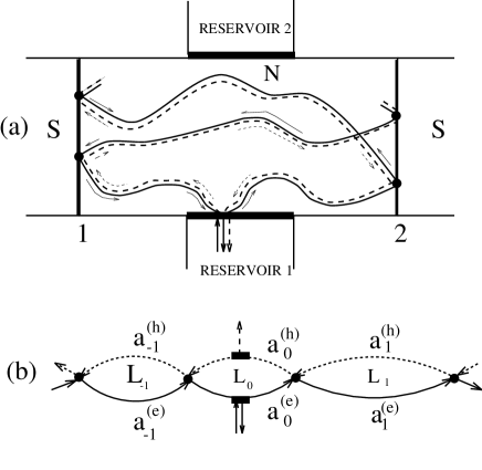
Figure 1: (a) Structure analyzed in the text, with superconducting (S) and disordered normal (N) elements labeled. The normal element is coupled to two reservoirs through tunnel barriers shown as thick black lines. Semiclassical trajectories of electron- and hole-like quasiparticle excitations are indicated by solid and dashed lines, respectively. Sections of the trajectories going between N/S boundaries 1 and 2 are connected by Andreev and normal reflections at the points shown as black dots. An electron incident from the resorvoir (solid up-arrow) may be reflected back either as an electron (solid down-arrow) or as a hole (dashed arrow). (b) Sequence of scattering events along the trajectory shown in (a). $L_{n}$ is the length of the trajectory in section $n$; $a_{n}^{(e,h)}$ are the amplitudes of the corresponding electron and hole excitations at the Fermi energy ($n=0,\pm 1,\ldots$).

2 Formulation of the problem

Figure 1 shows the geometry of the sample under consideration. A mesoscopic normal region in contact with two superconductors is coupled to two reservoirs of normal electrons through tunneling potential barriers of low transparency. The quasiparticle motion in the normal region is assumed to be affected by a smoothly varying disorder potential and is treated semiclassically.

According to the Landauer-Lambert formula [6] the conductance of the system corresponding to a current between two normal electron reservoirs can be written in terms of the probability $R_{a}(E)$ for electrons impinging from one reservoir with energy $E$ to be reflected as holes back into the same reservoir and in terms of the probability $T_{o}(E)$ for them to be transmitted to the other reservoir as electrons. For the case of two equal barriers one has

$$G=\frac{2e^{2}}{h}\int\left(-\frac{\partial f_{0}(E)}{\partial E}\right)\left(T_{0}(E)+R_{a}(E)\right)dE\,,$$ (1)

where $f_{0}(E)$ is the Fermi distribution function. Our objective is to calculate the ”electron-hole transmission” probability $R_{a}(E)$ in Eq. (1). This is sufficient, since it can be shown that due to the destructive interference among the relevant trajectories, $T_{0}(E)$ is only weakly affected by the superconductor phase difference $\phi$. Hence the effective transmission probability $T(E)$ for our problem, to be calculated below, is given by $R_{a}(E)$.

An electron impinging on the lower potential barrier in Fig. 1 from the reservoir gets, after possibly interacting with the barrier and the two S/N interfaces in the N-region, backscattered in the electron and hole channels with probability amplitudes $C^{(e)}_{{\bf p}}({\bf r}_{\parallel})$ and $C^{(h)}_{{\bf p}}({\bf r}_{\parallel}$) respectively. The coordinate ${\bf r}_{\parallel}=(0,y,z)$ lies in the plane of the barrier, the $x$-axis being perpendicular to the barrier plane. Accordingly, the wave function of the electron $u({\bf r}_{\parallel})$ and hole $v({\bf r}_{\parallel})$ in the reservoir can be written as

$$u({\bf r}) = {\rm e}^{i{\bf p}_{\parallel}{\bf r}_{\parallel}}\left({\rm e}^{ip_{x}^{(e)}x}+C^{(e)}_{{\bf p}}({\bf r}_{\parallel}){\rm e}^{-ip_{x}^{(e)}x}\right)$$

$$v({\bf r}) = {\rm e}^{i{\bf p}_{\parallel}^{(h)}{\bf r}_{\parallel}}C^{(h)}_{{\bf p}}({\bf r}_{\parallel}){\rm e}^{ip_{x}^{(h)}x}\,;\quad\quad\quad p_{x}^{(e,h)}=\sqrt{p_{F}^{2}-{\bf p}_{\parallel}^{(h)2}\pm E}$$ (2)

The probability for electron-hole transmission, which we need to calculate, is connected with the amplitude $C^{(h)}_{{\bf p}}({\bf r}_{\parallel})$ by the relation

$$T(E)=\frac{1}{(2\pi\hbar)^{2}}\int_{p_{\parallel}^{2}/2m\leq\epsilon_{F}}d{\bf p_{\parallel}}\int_{S}d{\bf r_{\parallel}}|C_{{\bf p}}({\bf r}_{\parallel})|^{2}\,,$$ (3)

where $S$ is the area of the tunnel barrier.

The wave function in the normal region N near the potential barrier is also characterized by electron and hole components,

$$u({\bf r}) = {\rm e}^{i{\bf p}_{\parallel}{\bf r}_{\parallel}}\left[A^{(e)}_{0}({\bf r}_{\parallel}){\rm e}^{ip_{x}^{(e)}x}+B^{(e)}_{0}({\bf r}_{\parallel}){\rm e}^{-ip_{x}^{(e)}x}\right]$$

$$v({\bf r}) = {\rm e}^{i{\bf p}_{\parallel}{\bf r}_{\parallel}}\left[A^{(h)}_{0}({\bf r}_{\parallel}){\rm e}^{ip_{x}^{(h)}x}+B^{(h)}_{0}({\bf r}_{\parallel}){\rm e}^{-ip_{x}^{(h)}x}\right]$$ (4)

A slowly varying potential in the N region (on the scale of the Fermi wavelength $\lambda_{F}$) is responsible for the semiclassical nature of the wavefunction (4) and the slow spatial variation of the factors $A^{(e,h)}({\bf r}_{\parallel})$ and $B^{(e,h)}({\bf r}_{\parallel})$. The matching conditions at the barrier, which can be expressed in terms of a unitary $2\times 2$ matrix, describe the coupling between $C^{(e,h)}({\bf r}_{\parallel})$ and $A^{(e,h)}({\bf r}_{\parallel})$, $B^{(e,h)}({\bf r}_{\parallel})$. We assume that these functions smoothly — in the semiclassical sense — go to zero at the perimeter of the injector reservoir and are equal to zero in the plane $x=0$ outside the injector.

Using the language of semiclassical propagation we now construct the wavefunction in the N-region (see Fig. 1) for the electron impinging on the lower barrier from the reservoir. We do so by mapping it to the wave function (2) at the injector barrier. Such a mapping is possible if the disorder potential does not cause any noticable divergence of a tube of trajectories with the transverse size of the order of $\lambda_{F}$ as they propagate for a certain length. In our case this characteristic length is the length covered by quasiparticle diffusing across the sample (see, e.g., [42]).

The procedure for doing the semiclassical mapping can be reduced to the following. For a given point ${\bf r}$ in the N region we have to introduce all different trajectories which connect this point with points on the barrier (where the momentum of the quasiparticle is $\bf p$), and experiencing all possible sequences of scatterings induced by N/S boundaries and barriers. According to Ref. [42], the semiclassical wavefunction can be constructed as a sum of partial contributions $\Psi_{n}$ corresponding to these trajectories, expressed in terms of the classical action $S_{l}=\int_{L_{l}}{\bf p}d{\bf l}$. As a result one has

$$u({\bf r}) = \sum_{l}A^{(e)}_{l}({\bf r})e^{iS_{l}^{(e)}/\hbar}$$

$$v({\bf r}) = \sum_{l}A^{(h)}_{l}({\bf r})e^{iS_{l}^{(h)}/\hbar}\,.$$ (5)

If a trajectory is split by interacting with a tunnel barrier or N/S interface, the wavefunction along that trajectory undergoes a transformation described by the scattering matrix already mentioned. The smoothly varying function $A^{(h)}_{l}({\bf r})$ can be found from the continuity equation for the current density, which together with the Hamilton-Jacobi equation for the action, guarantees that Eq. (5) is a solution of the Schrödinger equation [42]. Furthermore, one can readily verify that the wavefunction (5), constructed as a sum over trajectories, satisfies the boundary conditions corresponding to the scattering at the barriers and interfaces.

3 Electron-hole transmission at low energies

The wave function formally constructed in Eq. (5) does not permit us to carry out concrete calculations in a general case. The reason lies in the complications that arise due the bifurcations of trajectories as they undergo Andreev and normal reflections at the N/S boundaries. The situation is drastically simplified in the region of small energies, $E\ll E_{Th}$, where reflections in the Andreev channel send the quasiparticle back along the incident trajectory. This implies that the trajectory bifurcations disappear and the problem reduces to an analysis of one-dimensional quasiparticle motion along a single trajectory with centers for back (Andreev) and forward (normal) scattering.

A trajectory of this type is shown in Fig. 1. In this case the problem to find the wavefunction at the boundary [see Eq. (2)] is reduced to a quantum scattering problem for the configuration shown in Fig. 1b. The points of reflection at the N/S boundaries and the points of scattering at the tunnel barrier are shown with black dots and black bars, respectively. Propagation between these points is coherent in both electron and hole channels, which is illustrated by dashed and solid lines of equal lengths. For quasiparticles with finite energy $E$ the phase gains along the electron and hole trajectories do not completely cancel since the momenta are now different. The resulting decompensation effect is of order $E/E_{Th}$.

Wave functions in the adjacent sections of Fig. 1b are connected by a scattering matrix describing Andreev and normal reflections at the N-S boundary. The problem of evaluating the electron-hole transmission can now be formulated as follows. An electron in the reservoir arrives at the tunnel barrier (solid up-arrow in Fig. 1b), and we have to find the amplitude of the outgoing wave function in the hole channel (dashed up-arrow). This problem is reduced to solving a set of matching equations for amplitudes of electron $a_{n}^{(e)}$ and hole $a_{n}^{(e)}$ excitations in every section of propagation between scattering points. A further simplification follows as a consequence of the resonant transmission caused by multiple electron-hole transformations. Such a resonance occurs, as we will show, if the superconductor phase difference $\phi$ is close to an odd multiple of $\pi$ corresponding to a large number of trajectories contributing to a constructive interference between scattering events. If $|r_{N}|\ll 1$, where $r_{N}$ is the probability amplitude for non-Andreev (normal) reflection at an N/S boundary, the main contribution comes from trajectories wich do not include successive reflections at the same N/S boundary. Taking these observations into account the following set of algebraic matching equations emerge,

$$a_{0}^{{}^{(e)}} = r_{N}^{(2)}e^{i\Phi^{(e)}_{1}}a_{1}^{(e)}+(1-\frac{1}{2}\epsilon_{r})r_{A}^{(2)}e^{-i\Phi^{(h)}_{0}}a_{0}^{{}^{(h)}}$$

$$a_{1}^{{}^{(h)}} = -r_{A}^{(2)*}e^{i\Phi^{(e)}_{1}}a_{0}^{{}^{(e)}}+r_{N}^{(2)*}e^{-i\Phi^{(h)}_{0}}a_{0}^{{}^{(h)}}$$

$$a_{-1}^{{}^{(e)}} = r_{N}^{(1)}e^{i\Phi^{(e)}_{0}}a_{0}^{{}^{(e)}}+r_{A}^{(1)}e^{-i\Phi^{(h)}_{-1}}a_{-1}^{{}^{(h)}}$$

$$a_{0}^{{}^{(h)}} = -(1-\frac{1}{2}\epsilon_{r})r_{A}^{(1)*}e^{i\Phi^{(e)}_{0}}a_{0}^{{}^{(e)}}+r_{N}^{(1)*}e^{-i\Phi^{(h)}_{-1}}a_{-1}^{{}^{(h)}}-\sqrt{\epsilon_{r}}e^{i\Phi^{(e,1)}_{0}}$$ (6)

$$a_{1}^{{}^{(e)}} = r_{N}^{(1)}e^{i\Phi^{(e)}_{2}}a_{2}^{{}^{(e)}}+r_{A}^{(1)}e^{-i\Phi^{(h)}_{1}}a_{1}^{{}^{(h)}}$$

$$a_{2}^{{}^{(h)}} = -r_{A}^{(1)*}e^{i\Phi^{(e)}_{2}}a_{2}^{{}^{(e)}}+r_{N}^{(1)*}e^{-i\Phi^{(h)}_{3}}a_{3}^{{}^{(h)}}$$

$$\ldots = \ldots$$

The amount of phase gained after propagation along the trajectories in section $n$ is

$$\Phi^{(e,h)}_{n}(E)=\int_{L_{n}}p^{(e,h)}(E)dl/\hbar\approx\Phi_{n}\pm\tau_{n}E/\hbar\,,$$

where $\Phi_{n}=\Phi^{(e,h)}_{n}(0)$ and $\tau_{n}$ is propagation time in section n. The quantities $r_{A}^{(1,2)}$ and $r_{N}^{(1,2)}$ are, respectively, the probability amplitudes for Andreev and normal reflection at N/S boundaries 1 and 2. Phases and amplitudes of an electron or hole along the semiclassical paths are defined in such a way that no phase has been gained at the beginning of a particular electron or hole section $n$. Hence the amplitude is $a_{n}^{(e,h)}$ at the beginning of the section, and $a_{n}^{(e,h)}e^{\pm i\Phi^{(e,h)}_{n}}$ at its end. The phase gain between the tunnel barrier and the left N/S boundary (N/S boundary 1) is denoted by $\Phi_{0}^{(e,1)}$. In Eq.(6) a coefficient $\epsilon_{r}\ll 1$ characterizing the coupling through the tunnel barrier has furthermore been introduced. We note that one can show that the large phases $\Phi_{n}$ can be removed from the set of equations (6). This is a manifestation of the fact that the electron and hole phase gains compensate each other at $E=0$.

According to our construction the probability $|C_{{\bf p}}({\bf r}_{\parallel})|^{2}$ of an electron-hole transmission at the point ${\bf r}_{\parallel}$ of the barrier is related to the amplitude $a_{0}^{(h)}$ on the trajectory of Fig. 1 corresponding to injection at point ${\bf r}_{\parallel}$ as,

$$|C_{{\bf p}}({\bf r}_{\parallel})|^{2}=\epsilon_{r}|a_{0}^{(h)}|^{2}\,.$$ (7)

Equations (6) and (7) together with (3) give the complete solution for the oscillatory, $\phi$-dependent part of the excess conductance.

When $\epsilon_{r}=0$, Eq. (6) gives a set of Andreev levels $E_{\alpha}$. Therefore, one can expect that if $\epsilon_{r}\ll 1$ the trasmission probabilty $|C_{{\bf p}}^{(h)}({\bf r_{\parallel}})|^{2}$ is of the Breit-Wigner form. Indeed, as shown in Appedix 1, the transmission probability $|C_{{\bf p}}^{(h)}({\bf r_{\parallel}})|^{2}$ in this limit can be expressed as

$$|C_{{\bf p}^{(h)}({\bf r_{\parallel}})}|^{2}=\frac{4\epsilon_{r}^{2}E_{0}^{2}|a_{0,\alpha}^{(h)}|^{2}}{4(E-E_{\alpha})^{2}+\epsilon_{r}^{2}E_{0}^{2}}\,.$$ (8)

Here $E_{0}$ is the spacing of Andreev levels generated by the trajectory when $\epsilon_{r}=0$ and $n=0$, $a_{0,\alpha}^{(h)}$ is the solution of Eq. (6) for $E=E_{\alpha}$ and $\epsilon_{r}=0$. Because of the random variation of propagation times $\tau_{n}$, the functions $a_{0,\alpha}^{(h)}$ are localized along the one-dimensional ladder shown in Fig. 1b.

Further simplifications arise as one integrates the electron-hole transmission probability $|C_{{\bf p}}^{(h)}({\bf r_{\parallel}})|^{2}$ [see Eq. (3)] over the area of the injector area and over the the Fermi surface in momentum space. This integration corresponds to summing over different trajectories and one can think of it as averaging over various distributions of $\tau_{n}$. It follows that $T(E)$ can be expressed as

$$T(E)=N_{\perp}\left\langle\left\langle\frac{4\epsilon_{r}^{2}E_{0}^{2}|a_{0,\alpha}^{(h)}|}{4(E-E_{\alpha})^{2}+\epsilon_{r}^{2}E_{0}^{2}}\right\rangle\right\rangle\,,$$ (9)

where $N_{\perp}=Sp_{F}^{2}/h$, $S$ is the area of the injector and $\langle\langle\ldots\rangle\rangle$ implies an averaging over $\tau_{n}$. If $k_{B}T\gg\epsilon_{r}E_{0}$ one can neglect the width of the resonance for relevant energies, $E\sim kT$, and conclude that

$$T(E)=N_{\perp}\left\langle\left\langle\sum_{\alpha}\epsilon_{r}|a_{0,\alpha}^{(h)}|^{2}\delta([E-E_{\alpha}]/E_{0})\right\rangle\right\rangle\,.$$ (10)

The distribution of propagation times $\tau_{n}$ depends on the details of the disordered potential in the mesoscopic normal region. These are not known, but it is natural to assume that propagation times along different sections of the semiclassical trajectory (see Fig. 1a) are uncorrelated. Under this assumption one can, as detailed in Appendix 1, directly express the transmission probability $T(E)$ in terms of the average density of Andreev states coupled with the reservoir,

$$T(E)=N_{\perp}E_{Th}\left\langle\left\langle\nu(E)\right\rangle\right\rangle$$ (11)

with

$$E_{Th}=\left\langle\left\langle E_{0}\right\rangle\right\rangle=h\left\langle\left\langle\tau^{-1}\right\rangle\right\rangle\,.$$ (12)

Here $\nu(E)$ is the density of Andreev states generated by a given semiclassical trajectory when $\epsilon_{r}=0$.

In order to proceed with an analytical approach we choose a Lorentz form for the distribution function $P(\tau)$,

$$P(\tau)=\frac{1}{\pi}\frac{\gamma}{(\tau-\bar{\tau})^{2}+\gamma^{2}},$$ (13)

As shown in Appendix 2, this choice permits us to derive an analytical expression for the averaged density of state

$$\left\langle\left\langle\nu(E)\right\rangle\right\rangle=\frac{2|E|}{\pi}\int\limits_{-\infty}^{\infty}\frac{E_{1}^{2}\nu_{0}(E_{1})}{E_{1}^{4}+4E^{4}}dE_{1}$$ (14)

(we have used $\gamma=\overline{\tau}$, see [10]). The quantity $\nu_{0}(E)$ in the integrand of eq. (14) is the density of states of the periodic chain of Fig. 1b, if $\tau_{n}=\overline{\tau}$ for all $n$. It is straightforward to find this density of states to be

$$\nu_{0}(E)=\frac{2}{\pi}\frac{|E|}{\sqrt{(E^{2}-E_{\min}^{2})(E_{\max}^{2}-E^{2})}}\,,$$ (15)

The energies $E_{\min}$ and $E_{\max}$ are lower and upper edges of the energy band of the periodic chain of Fig. 1b. They can be expressed in terms of the “hopping integral” $r_{N}^{1,2}$ as

$$E_{\min,\max}=E_{Th}\sqrt{\delta\phi^{2}+\left(|r_{N}^{(1)}|\pm|r_{N}^{(2)}|\right)^{2}}\quad\delta\phi={\rm Min}|\phi-\pi(2k+1)|\,.$$ (16)

Finally, using Eqs. (1), (11 and 14) one finds that the low-temperature conductance can be expressed as

$$G = N_{\perp}\frac{2e^{2}}{h}\frac{\epsilon_{r}\sqrt{2}}{\overline{T}}\int_{0}^{\infty}\frac{x}{\cosh^{2}(x/2\overline{T})}\times$$

$$\ \left\{\frac{\sqrt{(4x^{4}+E_{min}^{4})(4x^{4}+E_{max}^{4})}+E_{min}^{2}E_{max}^{2}-4x^{4}}{(4x^{4}+E_{min}^{4})(4x^{4}+E_{max}^{4})}\right\}^{1/2}dx\,,$$

where $\overline{T}=T/T_{Th}$ with $T_{Th}=E_{Th}/k_{B}$ defined by Eq.(12).

The excess conductance $G(\phi)$ is plotted as function of phase difference in Fig. 2, while the maximum oscillation amplitude $G_{max}(T)$ is plotted as a function of temperature in Fig. 3. We emphasize two distinguishing features: 1) the excess conductance has sharp maxima at $\phi=\pi(2k+1),\;k=0,\pm 1,...$; 2) The peak oscillation amplitude has a maximum value for a temperature much below the Thouless temperature, $T\ll T_{Th}$, which qualitatively distinguish these results from those obtained for a completely transparant boundary between the mesoscopic region and the reservoirs. Without potential barriers between the reservoirs and the mesoscopic normal region there are no Andreev states that can contribute to the inter-reservoir transport. With such barriers present Andreev levels are well defined and long-lived. The peak of the conductance in Fig. 2 is due to resonant tunneling through a macroscopic number of such Andreev levels. A small amount of non-Andreev (normal) quasiparticle reflection at the N/S boundaries is not, as can be seen in Fig. 3, detrimental to the resonant tunneling effect. Rather it results in an energy shift of the position of the resonance (provided the probability for normal reflections at the two N/S boundaries are different). As a result the position of the maximum of the peak amplitude is shifted to a finite temperature, $T\sim\left||r_{N}^{(1)}|-|r_{N}^{(2)}|\right|T_{Th}$.

Figure 2: Normalized excess conductance $\Delta G(\phi)/G_{N}$ of the S/N/S structure shown in Fig. 1a as a function of the phase difference $\phi$ between the two superconductors. $\Delta G(\phi)\equiv G(\phi)-G(\phi=0)$, $G_{N}=\epsilon_{r}(2e^{2}/h)N_{\perp}$; $T/T_{Th}=0.1$, $r_{N}^{(1)}=0.1$, $r_{N}^{(2)}=0.2$

Figure 3: Temperature dependence of the maximum normalized excess conductance $\Delta G(\phi=\pi)/G_{N}$ for the same tunnel barrier parameters as in Fig. 2.

4 Conclusions

We have shown that resonant tunneling through Andreev levels may give rise to an excess quasiparticle contribution to the normal conductance of an S/N/S sample at energies much below the Thouless energy and with maximal amplitude when the phase difference between the superconductors is on odd multiple of $\pi$. That resonant tunnelling through Andreev levels could give rise to a “giant” effect was proposed for the case of a ballistic normal region in Ref. [9]. The effect discussed here is not sensitive to the details of the semiclassical motion of quasiparticles inside the disordered normal region. A more remarkable fact is that the main conclusion about the importance of resonant transmission through a macroscopically large number of Andreev levels seems to be valid not only for a smooth disorder potential allowing a semiclassical analysis to be carried out as done here. Indeed, one can consider the density of states in an S/N/S junction isolated from reservoirs and solve the Eilenberger-Usadel equation, which is valid for a short-range disorder potential in the normal region. This approach gives, according to Ref. [43], a gap in the spectrum which closes at $\phi=\pi$ with the density of states diverging at $E=0$.

In recent experiments [37, 41] oscillations of the conductance $G(\phi)$ have been observed, which are well described in the framework of the thermal effect of Nazarov and Stoof [7] at temperatures around the Thouless temperature, $T\sim T_{Th}$, but are significantly diferent from what the thermal effect can explain at lower temperatures. The conductance maxima were found to be $\pi$-shifted in both experiments in the range of low temperatures. The maximum oscillation amplitude $\Delta G(T)$ was observed at $T\approx 20$ mK (the Thouless temperature was $\approx 200$ mK [41]). One may speculate (see [41]) that grain boundaries and geometrical feauters of the contacts act to split the semiclassical quasiparticle trajectories in the same sense as the potential barriers in the model used here. If so one would expect the thermal effect [7, 8] and the resonant tunneling effect to co-exist. In this case the cross-over in the phase and temperature dependences of the conductance oscillations could be understood as a result of competition between the“high temperature” thermal effect and the “low temperature” resonant tunneling through Andreev levels.

Acknowledgment. Support from the Swedish KVA and NFR and from the National Science Foundation under Grant No. PHY94-07194 is gratefully acknowledged. MJ is grateful for the hospitality of the Institute for Theoretical Physics, UC Santa Barbara, where part of this work was done.

Appendix 1

The set of equations (6) can be re-arranged in the following way,

$$\left\{\widehat{\omega}(\varepsilon)+\epsilon_{r}\widehat{P}\right\}|a\rangle=\sqrt{\epsilon_{r}}|g^{(e)}\rangle\,.$$ (18)

Here $\widehat{\omega}(\varepsilon)=\widehat{1}-\widehat{U}(\varepsilon)$, $\widehat{1}$ is a unit matrix of order $2N\times 2N$ ($N$ is the number of sections in the chain in Fig. 1b), and $\widehat{U}(\varepsilon)$ is a $2N\times 2N$ unitary matrix whose explicit form can be found from Eq. (6) by setting $\epsilon_{r}=0$. The components of the vector $|a\rangle$ are the amplitudes $a_{n}^{(i)}$, where the subscript $n$ labels the sections of the chain ($n=0,\pm 1,\pm 2,...\pm N/2$); the superscript $i$ denotes the electron ($i=e$) and hole ($i=h$) paths, $\widehat{P}$ is an operator projecting onto the section of injection

$$\widehat{P}=(1/2)\left\{|g^{(e)}\rangle\langle g^{(h)}|-|g^{(h)}\rangle\langle g^{(e)}|\right\}\,.$$ (19)

The vector $|g^{(e)}\rangle$ has only one non-zero component $\delta_{n,0}\delta_{i,e}$ as has $|g^{(h)}\rangle$, $\delta_{n,0}\delta_{i,h}$ [see EQ. (6)]. The energy spectrum of a quasiparticle moving along the path of Fig. 1b in the absence of any coupling to the reservoirs is determined by the roots of the determinant of the matrix $\widehat{\omega}$. In order to find the resonant transmission amplitude we apply resonant perturbation theory to the set of algebraic equations (18) assuming the barrier transparency $\epsilon_{r}$ to be small ($\epsilon_{r}\ll 1$) and the energy $E$ of the incoming qusiparticle to be close to the energy level $E_{\alpha}$. Expanding the matrix $\widehat{\omega}(E)$ to lowest order in energy, $\widehat{\omega}(E)=\widehat{\omega}(E_{\alpha})+\widehat{\omega}^{{}^{\prime}}(E_{\alpha})\left(E-E_{\alpha}\right)$ and expanding the vector $|a\rangle$ to lowest order in the small parameter $\sqrt{\epsilon_{r}}$ as

$$|a\rangle=\gamma|e_{\alpha}\rangle+\sqrt{\epsilon_{r}}|a_{\alpha}^{(1)}\rangle,$$ (20)

one gets a set of algebraic equations,

$$\widehat{\omega}(E_{\alpha})|a_{\alpha}^{(1)}\rangle=-\gamma\left\{\left(E-E_{\alpha}\right)\widehat{\omega}^{{}^{\prime}}(E_{\alpha})+\epsilon_{r}\widehat{P}\right\}|e_{\alpha}\rangle+\sqrt{\epsilon_{r}}|g\rangle$$ (21)

where the vector $|e_{\alpha}\rangle$ is a normalized non-trivial solution of the equation

$$\widehat{\omega}(E_{\alpha})|e_{\alpha}>=0.$$ (22)

The constant $\gamma$ is determined by the condition that Eq. (21) has nontrivial solutions. Its value can be found by multiplying both sides of the set of equations with $\langle e_{\alpha}|$, the latter vector being a non-trivial solution of the set of equation,

$$\langle e_{\alpha}|\,\widehat{\omega}(E_{\alpha})=0$$ (23)

(the vectors $\langle e_{\alpha}|$ and $|e_{\alpha}\rangle$ are normalized in such a way that $\langle e_{\alpha}|e_{\alpha}\rangle=1$). As a result, one gets

$$\gamma=\frac{\sqrt{\epsilon_{r}}\langle e_{\alpha}|g^{(e)}\rangle}{\langle e_{\alpha}|\,\widehat{\omega}^{{}^{\prime}}(E_{\alpha})|e_{\alpha}\rangle\left(E-E_{\alpha}\right)+\epsilon_{r}\langle e_{\alpha}|\widehat{P}|e_{\alpha}\rangle}\,,$$ (24)

with $\langle e_{\alpha}|g^{(e)}\rangle=a^{e}_{0,\alpha}$. As we are considering the case of low normal reflection probability amplitudes, $|r_{N}^{(i)}|\ll 1$, and the terms in the denominator already contain small factors $\left(E-E_{\alpha}\right)$, the amplitudes $r_{N}^{(i)}$ can be neglected in these terms to lowest order. This gives as a result that $\langle e_{\alpha}|\widehat{\omega}^{{}^{\prime}}(E_{\alpha})|e_{\alpha}\rangle=i/E_{0}$ ($E_{0}=\hbar v_{F}/\tau_{0}$, $\tau_{0}$ is the propagation time along the path in the section of injection in Fig. 1b) and $\langle e_{\alpha}|\widehat{P}|e_{\alpha}\rangle=1/2$.

One can show that in the resonant approximation the second term on the right hand side of Eq. (20) can be neglected if the prameter $\epsilon_{r}\ll 1$. Hence the amplitude of the electron-hole transition is $a_{0}^{(h)}=\gamma\langle g^{(h)}|a\rangle$. Therefore, using Eq. (7) and (24) we get the Breit-Wigner formula (8).

5 Appendix 2

As shown by Slutskin [44], the density of states of a one-dimensional chain of the type in Fig. 1b can be written as a Fourier series,

$$\nu(E)=\frac{1}{hN}\sum\limits_{n=1}^{N}\tau_{n}\left(F_{n}+F_{n}^{*}+1\right)\,,$$ (25)

where

$$F_{n}=\sum\limits_{\{l_{m}\}}D(\{l_{n}\})\prod_{m}e^{il_{n}\tau_{m}E/\hbar}\,.$$

Here $\{l_{n}\}$ labels various sets of numbers $(l_{1,}l_{2,...}l_{N})$ where $l_{n=1}=1$ and $l_{m\not=n}$ is equal to 0 or 1; $D(\{l_{n}\})$ are Fourier coefficients which depend on the “hopping integrals” $r_{N}^{(1,2)}$. Since the “Fourier amplitudes” do not depend on $\tau_{n}$ one only has to average the product $\tau_{n}\prod_{n}{\rm e}^{il_{n}\tau_{n}E/\hbar}$ while calculating the average density of states. Using the Lorentzian distribution (13) one finds the result

$$\left\langle\left\langle\tau_{n}\prod_{m}{\rm e}^{il_{n}\tau_{m}E/\hbar}\right\rangle\right\rangle=\frac{\gamma}{\pi\overline{\tau}}\int\limits_{-\infty}^{\infty}dE_{1}\frac{E_{1}}{(E_{1}-E)^{2}+(\gamma/\overline{\tau})^{2}E^{2}}\left(\overline{\tau}\prod_{n}e^{il_{n}\overline{\tau}E_{1}/\hbar}\right)$$ (26)

The term in parenthesis in this expression is exactly the same as what appear on the right hand side of Eq. (25) provided the system in Fig.1b is periodic with all $\tau_{n}=\overline{\tau}$. From this and the fact that $\nu_{0}(E_{1})=\nu_{0}(-E_{1})$ the result Eq. (14) follows immediately.

References

- [1] B. Z. Spivak and D. E. Khmel’nitsky, Pis’ma Zh. Eksp. Teor. Fiz. 35, 334, (1982) [JETP Lett. 35, 412 (1982)]; B. L. Altshuler and B. Z. Spivak, ibid. 92, 609 (1987) [65, 343 (1987)]; B. Z. Spivak and A. Yu. Zyuzin, in Mesoscopic Phenomena in Solids Eds. B. L. Altshuler, P. A. Lee, and R. A. Webb (Elsevier, New York, 1991), p.37.
- [2] H. Nakano and H. Takayanagi, Solid State Commun. 80, 997, 1991; H. Nakano and H. Takayanagi, Phys. Rev. B 47, 7986, 1993.
- [3] V. T. Petrashov, V. N. Antonov, P. Delsing, T. Claeson, Phys. Rev. Lett., 70, 347, 1993.
- [4] F. W. J. Hekking and Yu. V. Nazarov, Phys. Rev. Lett., 71, 1625, 1993.
- [5] V. C. Hui and C. J. Lambert, Europhys. Lett., 23, 203, 1993.
- [6] C. J. Lambert, J. Phys.: Cond. Matter, 3, 6579, 1991; J. Phys.: Cond. Matter, 5, 707, 1993; C. J. Lambert, V. C. Hui, S. J. Robinson, J. Phys.: Cond. Matter, 5, 4187, 1993.
- [7] Yu. V. Nazarov and T.H. Stoof, Phys. Rev. Lett. 76, 823, 1996.
- [8] A. Volkov, N. Allsopp and C. J. Lambert, J. Phys.: Condens. Matter 8, L45, 1996;
- [9] A. Kadigrobov, A. Zagoskin, R. I. Shekhter and M. Jonson, Phys. Rev. B 52, R8662 (1995).
- [10] H. A. Blom, A. Kadigrobov, A. Zagoskin, R. I. Shekhter, and M. Jonson, Phys. Rev. B57, 9995 (1998).
- [11] H. Pothier, S Guéron, D Esteve, M. H. Devoret, Physica B 203, 226, 1994; H.Pothier, S. Guéron, D. Estève, and M. H. Devoret, Phys. Rev. Lett. 73, 2488 (1994).
- [12] B. J. van Wees, A. Dimoulas, J. P. Heida, T. M. Klapwijk, W.v.d. Graaf, G. Borghs, Physica B 203, 285 (1994).
- [13] P. G. N. de Vegvar, T. A. Fulton, W. H. Mallison, and R. E. Miller, Phys. Rev. Lett. 73, 1416 (1994).
- [14] Yu. V. Nazarov, Phys. Rev. Lett. 73, 1420, 1994.
- [15] (a) A.V. Zaitsev, Physica B, 203, 274 (1994); (b) A.V. Zaitsev, Phys. Lett. A 194, 315 (1994).
- [16] C. W. J. Beenakker, J. A. Melsen, and P. W. Brouwer, Phys. Rev. B 51, 13 883 (1995).
- [17] V. T. Petrashov, V. N. Antonov, P. Delsing, and T. Claeson, Phys. Rev. Lett. 74, 5268 (1995).
- [18] N. R. Claughton, M. Leadbeater, C. J. Lambert, V. N. Prigodin, cond-mat/9510117.
- [19] P. M. A. Cook, V. C. Hui and C. J. Lambert, Europhys. Lett. 30, 355 (1995).
- [20] N. K. Allsopp, J. Sánchez Cañizares, R. Raimondi and C. J. Lambert, J. Phys.: Condens. Matter 8, L377 (1996).
- [21] N. R. Claughton and C. J. Lambert, Phys. Rev. B 53, 6605, 1996.
- [22] N. R. Claughton, R. Raimondi, C. J. Lambert, Phys. Rev. B 53, 9310, 1996.
- [23] A. F. Volkov and A. V. Zaitsev, Phys. Rev. B 53, 9267, 1996.
- [24] L. C. Mur, C. J. P. M. Harmans, J. E. Mooij, J. F. Carlin, A. Rudra, M. Ilegems, Phys. Rev. B 54, R2327, 1996.
- [25] P. Charlat, H. Courtois, Ph. Gandit, D. Mailly, A. F. Volkov and B. Pannetier, Phys. Rev Lett. 77, 4950, 1996; H. Courtois, Ph. Gandit, D. Mailly and B. Pannetier, Phys. Rev Lett. 76, 130, 1996.
- [26] S. G. den Hartog, C. M. A. Kapteyn, B. J. van Wees, T. M. Klapwijk, W. van der Graaf, G. Borghs, Phys. Rev. Lett. 76, 4592, 1996.
- [27] R. Hubert et al. Phys. Rev. B 54, 14026, 1996.
- [28] S. Ohki, Y. Ootuka, J. Phys. Soc. Jpn. 65, 1917, 1996.
- [29] B. J. van Wees, H. Takayanagi in Mesoscopic Transport, Eds. L. P. Kouwenhoven, G. Schön, L. L. Schön (Kluwer, Dordrecht, The Nederlands, 19??).
- [30] F. Zhou, B. Spivak, cond-mat/9604185.
- [31] V. T. Petrashov, R. Sh. Shaikhaidarov, I. A. Sosin, Pis‘ma Zh. Eksp. Teor. Fiz. 64, 789 (1996).
- [32] B. J. van Wees, P. de Vries, P. Magnée, and T. M. Klapwijk, Phys. Rev. Lett. 69, 510 (1992).
- [33] V. T. Petrashov, R. Sh. Shaikhaidarov, I. A. Sosnin, P. Delsing and T. Claeson, (unpublished).
- [34] L. F. Chang, P. F. Bagwell, Phys. Rev. B 55, 12678 (1997).
- [35] P. Samuelsson, V. S. Shumeiko, and G. Wendin, Phys. Rev. B56, R5763 (1997).
- [36] H. Courtois, P. Gandit and B. Pannetier, D. Mailly, cond-mat/9810339.
- [37] E. Toyoda and H. Takayanagi, Physica B, 251), 472 (1998).
- [38] R. Hubert et al, Journal of Vacuum Science, 16, 1244 (1998).
- [39] A. F. Volkov, V. V. Pavlovskii, Usp. Fiz. Nauk, 168, 205 (1998).
- [40] C. J. Lambert and R. Raimondi, J. Phys.: Condens. Matter 10, 901 (1998).
- [41] A. Kadigrobov, L. Y. Gorelik, R. I. Shekhter, M. Jonson, R. Shaikhaidarov, V. T. Petrashov, P. Delsing, T. Claeson (unpublished).
- [42] P. A. M. Dirac, The Principles of Quantum Mechanics (Oxford, Clarendon Press, 1958).
- [43] F. Zhou, P. Charlat, B. Spivak, B. Pannetier, J. Low Temp. Phys. 110, 841 (1998).
- [44] A. A. Slutskin, Zh. Eksp. Teor. Fiz. 58, 1098 (1970) [Sov. Phys. JETP 31, 589 (1970)].