Mesoscopic superconductors under irradiation: Microwave spectroscopy of Andreev states

Abstract

We show that irradiation of a voltage-biased superconducting quantum point contact at frequencies of the order of the gap energy can remove the suppression of subgap dc transport through Andreev levels. Quantum interference among resonant scattering events involving photon absorption is furthermore shown to make microwave spectroscopy of the Andreev levels feasible. We also discuss how the same interference effect can be applied for detecting weak electromagnetic signals up to the gap frequency, and how it is affected by dephasing and relaxation.

1 Introduction

It is well known that the current through a voltage-biased superconducting quantum point contact (SQPC) is carried by localized states. These states, called Andreev states, are confined to the normal region of the contact. The energy of the states — the Andreev levels — exist in pairs, (one above and one under the Fermi level), and lie within the energy gap of the superconductor, with positions which depend on the change $\phi$ in the phase of the superconductors across the junction. The applied bias affects this phase difference through the Josephson relation, $\dot{\phi}=2eV/\hbar$. With a constant applied bias $V$ much smaller than the gap energy $\Delta$, $\phi$ will increase linearly in time, and the Andreev levels will move adiabatically within the gap. This motion is a periodic oscillation in $\phi$, indicating that no energy is transfered to the SQPC and a pure ac current will flow through the contact. This is actually the ac Josephson effect.

We wish to study this system in a non-equilibrium situation, one way to accomplish this is by introducing microwave radiation with a frequency $\omega\approx\Delta$, which will couple the Andreev levels to each other. The radiation will represent a non-adiabatic perturbation of the SQPC system. However, if the amplitude of the electromagnetic field is sufficiently small, the field will not affect the adiabatic dynamics of the system much unless the condition for resonant optical interlevel transitions is fulfilled. Such resonances will only occur at certain moments determined by the time evolution of the Andreev level spacing. The resonances will provide a mechanism for energy transfer to the system to be nonzero when averaged over time and hence for a finite dc current through the junction. The rate of energy transfer is in an essential way determined by the interference between different scattering events [1, 2], and therefore it is not surprising that oscillatory features appear in the (dc) current-voltage characteristics of an irradiated SQPC. Dephasing and relaxation will affect the interference pattern and may even conspire to produce a dc current flowing in the reverse direction with respect to the applied voltage bias. The mechanism behind this negative resistance is very similar to the one responsible for the “somersault effect” discussed by Gorelik et al. [3].

A peculiar feature of the Andreev bound states, in comparison with normal bound states, is that they can carry current. This is why microwave-induced transitions between Andreev levels can be detected by means of transport measurements. In fact, it is possible to do Andreev energy-level spectroscopy in the sense that the Andreev level spectrum at least in principle can be reconstructed from a measurement of the microwave-induced subgap current. Such microwave spectroscopy of Andreev states in mesoscopic superconductors is the topic addressed in this work.

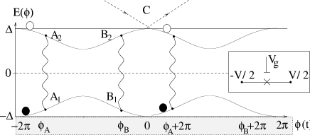
Figure 1: Time evolution of Andreev levels (full lines) in the energy gap of a gated voltage-biased, single-mode SQPC (see inset). A weak microwave field induces resonant transitions (wavy lines) between the levels at points $A$ and $B$ and the level above the Fermi energy becomes partly occupied to an extent determined by interference between the two transition amplitudes. Non-adiabatic interactions release the energy of quasiparticles in the (partly) occupied Andreev level into the continuum at point $C$, where the Andreev states and the continuum merge into each other (represented by dashed arrows, see text) and the initial conditions for the Andreev level populations are reset (filled and empty circles).

2 Theoretical framework

For an unbiased, mesoscopic SQPC — which by construction has a normal region $L$ which is much shorter than the coherence length $\xi_{0}$ — the Andreev spectrum of each transport mode has the form

$$E^{\pm}(\phi)=\pm E(\phi)=\pm\Delta[1-D\sin^{2}(\phi/2)]^{1/2}.$$ (1)

Here $D$ is the transparency of the mode and the energy is measured from the Fermi energy [4, 5]. With a small bias voltage applied, the levels move along the adiabatic trajectories $E^{\pm}(t)=\pm E(\phi_{0}+2eVt/\hbar)$ in energy-time space, oscillating with a period of $T_{p}=\hbar\pi/eV$, as shown in Fig. 1. In equilibrium the lower Andreev level will obviously be occupied, while the upper level will be empty. In the discussion below we consider a single-mode SQPC, although we note that the theory also applies for the case of a single dominant mode in a multi-mode junction. The transparency $D$ of the mode is taken to be arbitrary but energy-independent, $0<D<1$.

A high frequency electromagnetic field is applied to the gate situated near the contact, see inset in Fig. 1. The time-dependent electric field induced by the gate is concentrated within the non-superconducting region of the junction, and hence the charge carriers will couple to the electromagnetic field only there. When the criterion $\hbar\dot{\phi}=2eV\ll 2E^{2}(t)/\Delta$ for adiabaticity is obeyed, the rate of interlevel transitions is exponentially small keeping the level populations constant in time [6, 7]. The presence of a weak electromagnetic field [on the scale of $E(t)$] does not affect the adiabatic level trajectories except for short times close to the resonances at $t=t_{A,B}$, when $E(t_{A,B})=\hbar\omega/2$. Here the dynamics of the system is strongly non-adiabatic with a resonant coupling which effectively mixes the adiabatic levels. This is an analog of the well known Landau-Zener transition, which describes interlevel scattering as a resonance point is passed. In our case these transitions give rise to a splitting of the quasiparticle trajectory at the points $A,B$ into two paths; $A_{1}A_{2}B_{2}$ and $A_{1}B_{1}B_{2}$, forming a loop in $(E,t)$ space (see Fig. 1).

The resonant scattering opens a channel for energy absorption by the system; a populated upper level when approaching the edge of the energy gap (at point $C$ in Fig. 1) creates real excitations in the continuum spectrum, which carry away the accumulated energy from the contact. As a result, the net rate of energy transfer to the system is finite; it consists of energy absorbed both from the electromagnetic field and from the voltage source. The confluence of the two adiabatic trajectories at $B_{2}$ gives rise to a strong interference pattern in the probability for real excitations at the band edge, point $C$. The interference effect is controlled by the difference of the phases acquired by the system during propagation along the paths $A_{1}A_{2}B_{2}$ and $A_{1}B_{1}B_{2}$.

2.1 Bogoliubov-de Gennes equation

In order to describe the time evolution of the Andreev states in more detail we use the time-dependent Bogoliubov-de Gennes, (BdG), equation [8] for the quasiclassical envelopes $u_{\pm}(x,t)$ of the two-component wave function $\Psi(x,t)=u_{+}(x,t)e^{ik_{F}x}+u_{-}(x,t)e^{-ik_{F}x}$,

$$i\hbar\partial{\bf u}/\partial t=[{\bf H}_{0}+\sigma_{z}V_{g}(x,t)]{\bf u}\,.$$ (2)

In this equation ${\bf u}=(u_{+},u_{-})$ is a four-component vector, while ${\bf H}_{0}$ is the Hamiltonian of the electrons in the electrodes of the point contact,

$${\bf H}_{0}=-i\hbar v_{F}\sigma_{z}\tau_{z}\partial/\partial x+\Delta[\cos(\phi(t)/2)\sigma_{x}+i\sin(\phi(t)/2)\mbox{sgn}x\sigma_{y}],$$ (3)

where $\sigma_{i}$ and $\tau_{i}$ denote Pauli matrices in electron-hole space and in $u_{\pm}$ space respectively. For a mesoscopic junction the gap function $\Delta({\bf r})$ need not be calculated self-consistently, which is why in Eq. (3) it is assumed to have the constant value $\Delta\exp(i\phi/2)$ in the superconducting reservoir on one side of the SQPC and the different constant value $\Delta\exp(-i\phi/2)$ in the reservoir on the other side. The gate potential $V_{g}(x,t)=V_{\omega}(x)\cos\omega t$ in Eq. (2) oscillates rapidly in time and the amplitude is assumed to be small compared to the Andreev level spacing, $V_{\omega}\ll E(t)$.

The function ${\bf u}$, which is smooth on the scale of the Fermi wavelength, has a discontinuity at $x=0$, i.e. at the point contact, whose spatial extension can be neglected. The discontinuity translates to a boundary condition for ${\bf u}$,

$${\bf u}(+0)=(1/\sqrt{D})(1-\sqrt{R}\tau_{y}){\bf u}(-0),\;\;R=1-D,$$ (4)

which can be found [9] by matching at the point $x=0$ two scattering state solutions to the BdG equation approaching from left and right.

2.2 Resonant coupling of Andreev levels

Under the assumption that $eV,V_{g}\ll\Delta$ the system of Andreev levels experiences an adiabatic evolution in time. This is true at all times except close to the resonances (points $A$ and $B$ in Fig. 1) and at point C, which will be discussed later. For a resonant transition to occur, the deviation of the interlevel spacing from the resonance value $E(t)-\hbar\omega/2=\dot{E}(t_{A,B})\delta t$, where $\delta t$ is the duration of the resonance, has to be less than the quantum mechanical resolution of the energy levels $\hbar/\delta t$. Using this criterion we can estimate the duration $\delta t$ of the non-adiabatic evolution as $\delta t\sim[\hbar/\dot{E}(t_{A,B})]^{1/2}$, which implies that $\delta t$ is much shorter than the period $T_{p}=\hbar\pi/eV$ of Josephson oscillations if $eV\ll\Delta$. Hence, if this inequality is obeyed we may consider the non-adiabatic dynamics as temporally localized scattering events. We shall use this later to derive an analytical result for the induced dc current. For the time being, however, we will keep the discussion a little more general. We therefore introduce an Ansatz for the wave function u in the normal region of the junction in terms of a linear combination of the eigenstates ${\bf u}^{\pm}$ corresponding to the adiabatic Andreev levels $E^{\pm}$. The rapidly oscillating terms are explicitly introduced in this so called resonance approximation,

$${\bf u}(t)=b^{+}(t)e^{-i\omega t/2}{\bf u}^{+}+b^{-}(t)e^{i\omega t/2}{\bf u}^{-}\,.$$ (5)

Following Ref [3] we insert the Ansatz (5) into the BdG equation (2) to find, using the notation $\vec{b}=(b^{+},b^{-})$, an equation for the coefficients $b^{\pm}$,

$$i\dot{\vec{b}}(t)=\left[\begin{array}[]{cc}\delta\omega_{+-}(t)&V_{+-}/\hbar\\ V_{+-}^{\dagger}/\hbar&-\delta\omega_{+-}(t)\end{array}\right]\vec{b}(t).$$ (6)

Here $\delta\omega_{+-}(t)=[2E^{+}(t)-\hbar\omega]/2\hbar$ is a measure of the deviation from resonance. This equation describes the time evolution of the coefficients $b^{+}$ and $b^{-}$, which embody the dynamics of the population of the Andreev states under irradiation. We recall that the coupling to the time-dependent field is finite only in the normal region, which explains why $V_{+-}$ in (6) obtains as the matrix element of $\sigma_{z}V_{g}(x,t)$ between the Andreev states ${\bf u}^{\pm}$; $V_{+-}=(V_{\omega}/2)\int dx\langle{\bf u}^{+}\sigma_{z}{\bf u}^{-}\rangle$, where $\langle..\rangle$ denotes a scalar product in 4-dimensional space. For the case of a double barrier SQPC structure $V_{+-}$ was calculated in Ref. [3]. For a single barrier junction an analogous calculation gives us, $V_{+-}=\alpha(L/\xi_{0})\sqrt{DR}V_{\omega}\sin(\phi/2)$, where the constant $\alpha\sim 1$ is determined by the position of the barrier. We note, that this matrix element is proportional to the reflectivity of the junction; reflection mixes electron states with $+k_{F}$ and $-k_{F}$ allowing optical transitions between the Andreev levels. In a perfectly transparent SQPC ($D=1$), the upper and lower Andreev levels correspond to opposite electron momenta — the two levels cannot be coupled by radiation since momentum cannot be conserved — and the effect under consideration does not exist, cf. Refs. [6, 10].

2.3 Boundary conditions at $\phi=2\pi n$

Before we proceed to calculate the current through the irradiated SQPC we need to discuss the boundary condition at $\phi=2\pi n$ ($n$ is an integer). In the vicinity of these points, the Andreev levels approach the continuum and the adiabatic approximation is unsatisfactory, even at small applied voltages and weak electromagnetic fields. The duration $\delta t$ of the non-adiabatic interaction between the Andreev level and the continuum states can be estimated using the same argument as for the microwave-induced Landau-Zener scattering. One finds that, $\delta t\sim\hbar/(\Delta e^{2}V^{2})^{1/3}$. If we evaluate the condition, $\delta t<<T_{p}$, we find that we would require that $eV/\Delta\ll\pi^{3}$. This means that we can safely treat the non-adiabatic region as short. To derive the boundary condition, for example, at point $C$ in Fig. 1, one needs to calculate the transition amplitude connecting the states ${\bf u^{+}}(t_{1})$ at time $t_{1}\ll t_{C}-\delta t$ and ${\bf u^{+}}(t_{2})$ at time $t_{2}\gg t_{C}+\delta t$: $\langle{\bf u^{+}}(t_{2})\;{\bf U}(t_{2},t_{1}){\bf u^{+}}(t_{1})\rangle$. Here ${\bf U}(t_{2},t_{1})$ is the exact propagator corresponding to the Hamiltonian in Eq. (2). We will now proceed with symmetry arguments to show that this amplitude is exactly zero.

It can be shown that both the Hamiltonian (3) and the boundary condition for ${\bf u}$ at $x=0$ (4) are invariant under the simultaneous charge- and parity inversion described by the unitary operator ${\bf\Lambda}\equiv\hat{P}\sigma_{x}\tau_{z}$, where $\hat{P}$ is the parity operator in $x$-space. This implies that at any time any non-degenerate eigenstate of the Hamiltonian is an eigenstate of the symmetry operator ${\bf\Lambda}$ with eigenvalue $+1$ or $-1$ and that this property persists during the time evolution of the state. Specifically, if we take a state on each side of $\phi=0$,

$${\bf\Lambda}{\bf u}^{+}(\phi) = \lambda_{1}{\bf u}^{+}(\phi)$$ (7)

$${\bf\Lambda}{\bf u}^{+}(-\phi) = \lambda_{2}{\bf u}^{+}(-\phi).$$ (8)

Next we insert ${\bf u}^{+}(-\phi)=\Upsilon{\bf u}^{+}(\phi)$, where the operator $\Upsilon=\sigma_{x}\tau_{y}$ changes the sign of the phase $\phi$, into Eq. (8) and apply $\sigma_{x}\tau_{y}$ from the left and arrive at,

$${\bf\Lambda}{\bf u}^{+}(\phi)=-\lambda_{2}{\bf u}^{+}(\phi),$$ (9)

which shows that $\lambda_{1}=-\lambda_{2}$. This means that the two states, ${\bf u}^{+}(\phi)$ and ${\bf u}^{+}(-\phi)$ are orthogonal. This is consistent with the results of Shumeiko et.al. [9], who have shown that the Andreev state wave functions are $4\pi$-periodic whereas the energy levels and the current are $2\pi$-periodic. Since the state evolving from the adiabatic state ${\bf u^{+}}(t_{1})$ is orthogonal to the adiabatic state ${\bf u^{+}}(t_{2})$, the probability for an adiabatic Andreev state to be “scattered” into a localized state after passing the non-adiabatic region is identically zero. In reality, the Andreev state as it approaches the continuum band edge decays into the states of the continuum. Such a decay corresponds to a delocalization in real space and is the mechanism for transferring energy to the reservoir [11].

The orthogonality property shown above guarantees that the coherent evolution of our system persists during only one period of the Josephson oscillation and that the equilibrium population of the Andreev levels is reset at each point $\phi=2\pi n$ [12]. This imposes the boundary condition

$$b^{+}(2\pi n+0)=0,\;b^{-}(2\pi n+0)=1,$$ (10)

at the beginning of each period.

2.4 Calculation of the current

The quasiclassical equation for the total time dependent current at the junction ($x=0$) reads $I(t)=-ev_{F}\langle{\bf u}\tau_{z}{\bf u}\rangle\mid_{x=0}$. By manipulating the BdG equation as given by (2) and (3) and omitting oscillating terms which will not contribute to the dc current — the quantity of interest — one may turn this expression into the following form,

$$I(t)=\frac{2e}{\hbar}\left({d\phi\over dt}\right)^{-1}\int^{\infty}_{-\infty}dx\left[i\hbar\frac{d\langle{\bf u}\dot{\bf u}\rangle}{dt}-\dot{V}_{g}\langle{\bf u}\sigma_{z}{\bf u}\rangle\right].$$ (11)

In the static limit, $\dot{V}_{g}=0$ and $\dot{\phi}\rightarrow 0$, this result is clearly equivalent to the standard expression $I=(2e/\hbar)\,(dE^{\pm}/d\phi)$ for the Andreev level current.

In the general nonstationary case ${\bf u}$ is a linear combination of ${\bf u}^{\pm}$ according to Eq. (5) and we can calculate the current averaged over the period $T_{p}$. This is done through Eq. (11) with help of Eq.( 6) and the normalization condition $|b^{+}|^{2}+|b^{-}|^{2}=1$, leading to

$$I_{dc}={2e\over\pi\hbar}\left(\Delta-{\hbar\omega\over 2}\right)\left[|b^{+}(T_{p})|^{2}-|b^{+}_{0}|^{2}\right],$$ (12)

where $|b^{+}(T_{p})|^{2}$ is the population of the upper level at the end of the period and $|b^{+}_{0}|^{2}$ at the beginning of the period. The result simplifies further since according to Eq. (10) $|b^{+}_{0}|^{2}=0$.

The direct current through the contact can be viewed as resulting from photon-assisted pair tunneling or equivalently as being due to the distortion of the ac pair current due to the induced interlevel transitions. To facilitate an understanding of the current expression in another way, let us study energy conservation. We have two sources of energy, the applied field and the applied bias. If we consider a single Josephson period $T_{p}$, the energy absorbed by the system from the voltage source is $I\cdot V\cdot T_{p}$, and from the applied field it is $\hbar\omega|b^{+}(T_{p})|^{2}$ (assuming for simplicity that $|b^{+}_{0}|^{2}=0$). Energy conservation for the period can be stated as, $E_{out}=E_{absorbed}$, with the energy leaving the system stated as $2\Delta|b^{+}(T_{p})|^{2}$:

$$2\Delta|b^{+}(T_{p})|^{2}=I\cdot V\cdot T_{p}+\hbar\omega|b^{+}(T_{p})|^{2}.$$ (13)

The current can then easily be found as,

$$I=\frac{1}{VT_{p}}(2\Delta|b^{+}(T_{p})|^{2}-\hbar\omega|b^{+}(T_{p})|^{2})$$ (14)

or, inserting the value of $T_{p}$,

$$I=\frac{2e}{\hbar\pi}(\Delta-\frac{\hbar\omega}{2})|b^{+}(T_{p})|^{2}.$$ (15)

This is exactly the same result as obtained by the more tedious method used above. This discussion allows us to interpret the current as voltage-bias mediated, photon assisted tunneling.

3 Results of numerical and analytical analysis

Generally the current is given by Eq. (12) with the boundary condition Eq. (10) inserted. The actual calculation of the current has to be done numerically in most cases. However, in the limit of a weak applied external field and when the frequency of the applied field is such that we have two (in time) well separated resonances, we can treat the resonances as temporally localized scattering events. This approach can be quite rewarding as will become clear below.

3.1 Scattering formalism

Formally, we can describe the system’s evolution through a resonance by letting a scattering matrix $\hat{S}$ connect the coefficients $b^{\pm}$ before and after the splitting points $A$ and $B$. Approximating the time dependence of the Andreev levels to be linear, a standard analysis of the Landau-Zener interlevel transitions (see e.g. [3]) gives the scattering matrix elements at the points $A$ and $B$ as,

$$\hat{S}_{A}=\left[\begin{array}[]{cc}r&-de^{-i\Theta}\\ de^{i\Theta}&r\end{array}\right],\hat{S}_{B}=\left[\begin{array}[]{cc}r&de^{i\Theta}\\ -de^{-i\Theta}&r\end{array}\right],$$ (20)

where $|d|^{2}=1-|r|^{2}=1-e^{-\gamma}$ is the probability of the Landau-Zener interlevel transition. Here $\gamma=\pi|V_{+-}|^{2}/|dE/dt|$ where $V_{+-}$ is once again the matrix element for the interlevel transitions.

By introducing the matrix $\hat{\Phi}_{j,i}=\exp{(i\sigma_{z}\Phi(i,j))}$,

$$\Phi(i,j)={1\over 2eV}\int_{\phi_{i}}^{\phi_{j}}d\phi\left(E(\phi)-{\hbar\omega\over 2}\right),$$ (21)

which describes the “ballistic” dynamics of the system between the Landau-Zener scattering events, we connect the coefficients $b^{\pm}$ at the end of the period of the Josephson oscillation, $\phi=0$, with the coefficients $b^{\pm}_{0}$ at the beginning of the period, $\phi=-2\pi$,

$${b^{+}\choose b^{-}}=\hat{\Phi}_{0,B}\hat{S}_{B}\hat{\Phi}_{B,A}\hat{S}_{A}\hat{\Phi}_{A,-2\pi}{b^{+}_{0}\choose b^{-}_{0}}.$$ (22)

The time-averaged current through the junction can be directly expressed through these coefficients. Combining the boundary condition (10) with Eqs. (12) and (22), one finds

$$I_{dc}={8e\over\pi\hbar}\left(\Delta-{\hbar\omega\over 2}\right)e^{-\gamma}(1-e^{-\gamma})\sin^{2}(\Phi(A,B)+\theta),$$ (23)

where $\theta$ is the phase of the probability amplitude for the Landau-Zener transition, which only weakly depends on $V$. In Fig. 2 the current is calculated both numerically and with the expression above, Eq. (23). The current is plotted as a function of inverse voltage in order to show a periodicity in $1/V$. The close fit in Fig. 2 ensures us that the scattering approach works well for the situation when the resonances are well separated and the applied field is weak.

Figure 2: Current vs. inverse voltage from Eq. (15) for a biased SQPC irradiated with microwaves of frequency $\omega=1.52\Delta/\hbar$ and amplitude corresponding to a matrix element $|V_{+-}|=0.024\Delta$ for interlevel transitions, $I_{c}=e\Delta D/\hbar$. Note the cut in the inverse voltage scale. Results of the scattering approach, Eq. (19) [$\diamond$], are close to those obtained by numerically solving the BdG-equation with the radiation field treated in the resonance approximation (solid line). The close fit means that the scattering picture can be used to reconstruct the Andreev levels from the period of the current oscillations (Andreev level spectroscopy, see Section 3.2).

3.2 The quantum point contact as an interferometer

Equation (23) is the basis for presenting the biased SQPC as a quantum interferometer. There is a clear analogy between the SQPC interferometer and a standard SQUID in that they both rely on the presence of trajectories that form a closed loop. In a SQUID, which is used to measure magnetic fields, the loop is determined by the device geometry; in the SQPC the voltage (analog of the magnetic field) is well defined while the “geometry” of the loop in $(E,t)$ space can be measured. This loop is determined by the Andreev-level trajectories in $(E,t)$ space and is controlled by the frequency of the external field. This gives us an immediate possibility to reconstruct the phase dependence of the Andreev levels from the frequency dependence of the period $\Pi$ of oscillations of the current versus inverse voltage, see Fig. 2. Indeed, it follows from Eq. (21), that

$$\phi(E)=\pi\pm{4\pi e\over\hbar}\left.{d\Pi^{-1}\over d\omega}\right|_{\omega=2E}.$$ (24)

This shows that the position of the Andreev energy levels can be reconstructed from measurements of microwave-induced subgap currents through the SQPC.

4 Discussion - dephasing and relaxation

In order to be able to do interferometry it is necessary to keep phase coherence during at least one period of the Josephson oscillation. There are three dephasing mechanisms that impose limitations in practice: (i) deviations from an ideal voltage bias, (ii) microscopic interactions, and (iii) radiation induced transitions to continuum states. The main source of fluctuations of the applied voltage is the ac Josephson effect. According to the RSJ model, a fixed voltage across the junction can only be maintained if the ratio between the intrinsic resistance $R_{i}$ of the voltage source and the normal junction resistance $R_{N}$ is small. If $R_{i}/R_{N}\ll 1$ the amplitude of the voltage fluctuations $\delta V$ is estimated as $\delta V\sim(R_{i}/R_{N})\Delta$. Effects of voltage fluctuations on the accumulated phase $\Phi(A,B)$ can be neglected if $\delta\Phi(A,B)=\Phi^{\prime}(A,B)\delta V\ll 2\pi$, i.e. if $eV>(R_{i}/R_{N})^{1/2}\Delta$, which corresponds to a lower limit for the bias voltage [13].

The dephasing time due to microscopic interactions is comparable to the corresponding relaxation time [14]. This mechanism of dephasing can be neglected as soon as the relaxation time exceeds the Josephson oscillation period, $\tau_{i}\gg\hbar\pi/eV$. Taking electron-phonon interaction as the leading mechanism of inelastic relaxation, we estimate $\tau_{i}$ to be of the order of the electron-phonon mean free time at the critical temperature, $\tau_{ph}(T_{c})$, since the large deviations from equilibrium in our case occur in the energy interval $E<\Delta$. This gives [15] another limitation on how small the applied voltage can be, $eV>10^{-2}\Delta$.

The third mechanism of dephasing becomes important when the Andreev levels are closer than $\hbar\omega$ to the continuum band edge. One can estimate the corresponding relaxation time as $\tau_{\omega}\sim\hbar\Delta/V^{2}_{\omega}$. For small radiation amplitudes $\tau_{\omega}$ exceeds $T_{V}$, while for optimal amplitudes they are about equal. The effect of the level-continuum transitions on the interference oscillations depends on the frequency. If $\hbar\omega<2\Delta/3$ the “loop region” [$E(t)<\hbar\omega/2$] is optically disconnected from the continuum, and transitions cannot destroy interference. Possible level-continuum transitions at times outside the loop will only decrease the amplitude of the effect by a factor $\exp(-\alpha V_{\omega}^{2}/eV\Delta)$, where $\alpha<1$ is the relative fraction of the period $T_{V}$ during which transitions to the continuum are possible. Accordingly, this factor is of the order of unity for the voltages that correspond to the maximum amplitude of oscillations. If $\hbar\omega>2\Delta/3$, the interference is impeded by the optical transitions into the continuum, and the current oscillations decrease. Still, a nonzero average current through the junction will persist.

In any real system, both relaxation and dephasing will be present as discussed above. Therefore, to complete our analysis we will simulate these effects on our system. If we assume that the relaxation and dephasing times, $\tau,\tau_{\phi}$ are long compared to the duration of the non-adiabatic resonances, $\delta t$, we can use a technique [14], where dissipation is modelled by adding a term to the time evolution equation of the density matrix for the two-level Andreev system. The equations are, where relaxation enters in the diagonal terms and dephasing through the off-diagonal terms,

$$\dot{\rho}_{nn}(t)=-\frac{i}{\hbar}[H_{0}(t),\rho(t)]_{nn}-\frac{\rho_{nn}-\rho_{nn}^{eq}}{\tau},$$ (25)

$$\dot{\rho}_{nn^{\prime}}(t)=-\frac{i}{\hbar}[H_{0}(t),\rho(t)]_{nn^{\prime}}-\frac{\rho_{nn^{\prime}}}{\tau_{\phi}},\;\mbox{n$\neq$n'}.$$ (26)

with $\tau$ as the characteristic time for relaxation of the system to the equilibrium population, $\rho^{eq}$ and $\tau_{\phi}$ as the characteristic time for dephasing. These equations describe the “ballistic” dynamics of the dissipative system, replacing Eq. (21).

The exact form of the density matrix for the system considered here will be a $2{\times}2$ matrix for the discrete two level space of the Andreev states. (To avoid confusion we will use $\sigma_{1},\sigma_{2},\sigma_{3}$ to denote the Pauli matrices in this discrete space.) The Hamiltonian for the density matrix is found in Eq. (6), and the diagonal elements $\rho_{11}$ and $\rho_{22}$ will represent the population of the upper and lower Andreev levels. The resonant events which are unaffected by the dissipation can still be modeled with the scattering matrices introduced earlier, Eq. (20),

$$\rho^{\prime}=\hat{S}_{A,B}\;\rho\;\hat{S}_{A,B}^{\dagger}.$$ (27)

To calculate the effect of relaxation and dephasing on the current we will use the standard expression, $I=2e/\hbar(\partial E/\partial\phi)$, for the current carried by a populated Andreev state and average over one Josephson period. The result is, as a function of the upper levels population,

$$I_{dc}^{diss}=\frac{1}{T_{p}}\int_{0}^{T_{p}}I(t)dt=\frac{1}{T_{p}}\frac{2e}{\hbar}\int_{0}^{T_{p}}Tr(\sigma_{3}\rho)\partial E/\partial\phi\;dt=\frac{1}{T_{p}V}\int_{0}^{T_{p}}\frac{\partial E^{+}(t)}{\partial t}\left[2\rho_{11}-1\right]dt,$$ (28)

where we have used the Josephson relation $\dot{\phi}=2eV/\hbar$ and the conservation of probability, $Tr(\rho)=1$.

By solving the time evolution equations of the density matrix for the whole Josephson period and imposing the boundary condition $\rho(0)=\rho^{eq}=(1-\sigma_{3})/2$ ,we arrive at the following result,

$$\raggedleft\rho_{11}=\left\{\begin{array}[]{lll}0&\mbox{, $0<t<t_{1}$}&\\ d^{2}\;e^{-(t-t_{1})/\tau}&\mbox{, $t_{1}<t<t_{2}$}&\\ f(r^{2},\tau_{\phi},\tau)\;e^{-(t-t_{2})/\tau}&\mbox{, $t_{2}<t<T_{p}$}&\end{array}\right.\@add@raggedleft$$ (32)

where

$$f(r^{2},\tau_{\phi},\tau)=\left[d^{2}(1-e^{-(t_{2}-t_{1})/\tau})+2r^{2}d^{2}(e^{-(t_{2}-t_{1})/\tau}-e^{-(t_{2}-t_{1})/\tau_{\phi}}\cos{2(\Phi(A,B)+\Theta)})\right].$$ (33)

Inserting these expressions into Eq. (28) we find,

$$I_{dc}^{diss}(V)=\frac{2}{VT_{p}}\left[\frac{d^{2}\hbar\omega}{2}\left(e^{-(t_{2}-t_{1})/\tau}-1\right)+\frac{d^{2}}{\tau}\int_{t_{1}}^{t_{2}}E^{+}(t)dt+\right.$$

$$\left.f(r^{2},\tau_{\phi},\tau)\left\{\left(\Delta e^{-(T_{p}-t_{2})/\tau}-\frac{\hbar\omega}{2}\right)+\frac{1}{\tau}\int_{t_{2}}^{T_{p}}E^{+}(t)e^{-(t-t_{2})/\tau}dt\right\}\right].$$

The first important property of this expression is that for $\tau_{\phi}\rightarrow\infty$ and $\tau\rightarrow\infty$ it reduces to the previous current expression that we derived, Eq. (23). One obvious effect on the current is that the oscillations of the current decrease when the dephasing time, $\tau_{\phi}$, becomes small. Another is that when the relaxation time, $\tau$, is decreased, the current diminishes, see Fig. 3.

We note that the number of parameters has become quite large. It is now possible to calculate the current for different combinations of $\tau,\tau_{\phi},V,V_{+-},\omega,$ and the transmission coefficient $D$.

A curious effect occurs when the relaxation time is such that the upper level, after being populated at point A, is fully depopulated at $\phi=\pi$, the middle of the Josephson period. What we find is a negative dc current for a positive bias, a regime where our system shows a negative conductance, see Fig. 3, plots a and d. The relaxation time is such that the upper level is mainly populated when it’s derivative is negative (it carries a negative current) and then the lower level is highly populated for the part of the period when it’s derivative is negative. This effect will be most pronounced when the energy of the applied field, $\hbar\omega$, approaches the energy of the gap, $2\Delta$, as in Fig. 3d.

Actually, the physical mechanism which is behind the appearance of this negative resistance is similar to the one responsible for the “somersault effect” effect discussed in Ref. [3]. In that case the method for periodically bringing a pair of Andreev levels in a superconducting quantum point contact in resonance with a microwave field was different. Rather than applying a voltage bias, the time-dependence of the gate potential was assumed to have two components; one slow component which shifts the Andreev levels through its effect on the transparency $D=D(k_{F}(t))$ and one fast (microwave) component for coupling the two levels.

Figure 3: Simulations of the current when relaxation and dephasing are added. In a) only relaxation is added, with $\tau\approx 2\cdot 10^{-10}$s, the average value of the current decreases and also may become negative. In b) there is only dephasing, with $\tau_{\phi}\approx 5\cdot 10^{-10}$s. In c) both types of dissipation are added with $\tau=\tau_{\phi}\approx 5\cdot 10^{-10}$s. When, as in d), the frequency of the applied field is increased such that it approaches the superconductor energy gap, $2\Delta$, we find that the system shows a negative conductance, see text, when $\tau=\tau_{\phi}\approx 2\cdot 10^{-10}$s. For plots a,b,c $\hbar\omega/2\Delta\approx 0.75$ and for plot d $\hbar\omega/2\Delta\approx 0.95$. The amplitude of the external field is such that $|V_{+-}|/\Delta=0.024$ in all plots, and for reference the case when $\tau\rightarrow\infty$ and $\tau_{\phi}\rightarrow\infty$ are included (dotted curves).

5 Conclusions

We have shown that irradiation of a voltage-biased superconducting quantum point contact at frequencies $\omega\sim\Delta$ can remove the suppression of subgap dc transport through Andreev levels. Quantum interference among resonant scattering events can be used for microwave spectroscopy of the Andreev levels.

The same interference effect can also be applied for detecting weak electromagnetic signals up to the gap frequency. Due to the resonant character of the phenomenon, the current response is proportional to the ratio between the amplitude of the applied field and the applied voltage, $I\sim|V_{\pm}|^{2}/\Delta eV$. At the same time, for common SIS detectors a non-resonant current response is proportional to the ratio between the amplitude and the frequency of the applied radiation [16]), $I\sim|V_{\pm}/\omega|^{2}$, i.e. it depends entirely on the parameters of the external signal and cannot be improved.

Finally, we note that the classic double-slit interference experiment, where two spatially separated trajectories combine to form an interference pattern, clearly demonstrates the wave-like nature of electron propagation. For a 0-dimensional system, with no spatial structure, we have shown that a completely analogous interference phenomenon may occur between two distinct trajectories in the temporal evolution of a quantum system.

Acknowledgment. Support from the Swedish KVA, SSF, Materials consortia 9 & 11, NFR and from the National Science Foundation under Grant No. PHY94-07194 is gratefully acknowledged. NIL and MJ are grateful for the hospitality of the Institute for Theoretical Physics, UC Santa Barbara, where part of this work was done.

References

- [1] L. Y. Gorelik, N. I. Lundin, V. S. Shumeiko, R. I. Shekhter, and M. Jonson, Phys. Rev. Lett. 81, 2538 (1998).
- [2] The role of photoinduced interference effects in a normal junction was discussed by L. Y. Gorelik, A. Grincwajg, V. Kleiner, R. I. Shekhter, and M. Jonson, Phys. Rev. Lett. 73, 2260 (1994); L. Y. Gorelik, F. Maaø, R. I. Shekhter, and M. Jonson, Phys. Rev. Lett. 78, 3169 (1997).
- [3] L. Y. Gorelik, V. S. Shumeiko, R. I. Shekhter, G. Wendin and M. Jonson, Phys. Rev. Lett. 75, 1162 (1995).
- [4] A. Furusaki and M. Tsukada, Physica B 165-166, 967 (1990).
- [5] C. W. J. Beenakker, Phys. Rev. Lett. 67, 3836 (1991).
- [6] D. Averin and A. Bardas, Phys. Rev. Lett. 75, 1831 (1995); Phys. Rev. B 53, R1705 (1996).
- [7] E. N. Bratus’, V. S. Shumeiko, E. V. Bezuglyi, and G. Wendin, Phys.Rev. B 55, 12666 (1997).
- [8] P. G. de Gennes, Superconductivity of Metals and Alloys (Addison-Wesley, New York, 1966).
- [9] V. S. Shumeiko, G. Wendin, and E. N. Bratus’, Phys. Rev. B 48, 13129 (1993); V. S. Shumeiko, E. N. Bratus’, and G. Wendin, Low Temp. Phys. 23, 181 (1997).
- [10] U. Gunsenheimer and A. Zaikin, Europhys. Lett. 41, 195 (1998).
- [11] This conclusion is in agreement with the analysis of multiple Andreev reflections in Ref. [7].
- [12] This result is obvious for a pure SNS contact () since the two Andreev states involved in the transition at the band edge have momenta and pointing in opposite directions. See also [6].
- [13] Shunting by the junction capacitance is small at relevant frequences () if .
- [14] E. Shimshoni and Y. Gefen, Ann. Phys. 210, 16 (1991).
- [15] S. Kaplan, C. Chi, D. Langenberg, J. Chang, S. Jafaney, and D. Scalapino, Phys. Rev. B 14, 4854 (1976).
- [16] J. R. Tucker and M. J. Feldman, Rev. Mod. Phys. 57, 1055 (1985).