Electro-Mechanical Fredericks Effects in Nematic Gels

Abstract

The solid nematic equivalent of the Fredericks transition is found to depend on a critical field rather than a critical voltage as in the classical case. This arises because director anchoring is principally to the solid rubbery matrix of the nematic gel rather than to the sample surfaces. Moreover, above the threshold field, we find a competition between quartic (soft) and conventional harmonic elasticity which dictates the director response. By including a small degree of initial director misorientation, the calculated field variation of optical anisotropy agrees well with the conoscopy measurements of Chang et al (Phys. Rev. E56, 595 (1997)) of the electro-optical response of nematic gels.

PACS: 61.30.-v, 78.20.Jq, 82.70.Gg

I Introduction

In nematic elastomers and gels, liquid crystal ordering and the nematic director are coupled to the mechanical degrees of freedom. Both symmetric shear strains and antisymmetric deformations couple to the director. Since the macroscopic shape of the polymer network naturally depends on the chain anisotropy direction, the coupling gives rise to some remarkable features of the elasticity: shape can change spontaneously by well over 50% on changing temperature through the clearing point, shears can induce director rotation, and some shear deformations cost no change in energy in the ideal case. We call this last effect “soft elasticity”. It is unique to nematic networks and other elastic solids where a non-elastic internal degree of freedom is coupled to the mechanical degrees of freedom. The additional symmetries leading to softness were predicted phenomenologically by Golubovic and Lubensky [1] and from statistical mechanics of large deformations by Bladon et al [2]. Depending on the thermo-mechanical history, nematic elastomers have been shown to demonstrate either extreme softness or substantial deviations from soft response [3]. Systems with such residual resistance to deformation have been called semi-soft [4]. They are qualitatively like soft elastomers in that the same particular modes of non-trivial deformation cost a very small elastic energy, compared to other non-specific deformations.

Conventional nematics couple strongly to electric fields (${\rm\bf E}$), the director aligning parallel to the field in the case of positive dielectric anisotropy $\Delta\varepsilon$. When the director is anchored at boundaries and the sample is uniformly aligned perpendicular to the direction to be taken by the electric field, there is a transition (Fredericks) at a finite critical voltage, $V_{F}$, above which the director is deflected by the field. The electric Fredericks effect and its analogues are the basis of most liquid crystalline displays. Director rotation to lower the dielectric energy in the bulk becomes non-uniform if the boundary anchoring of the director is to be respected. In this case the Frank elastic energy density $\frac{1}{2}K(\nabla{\rm\bf n})^{2}$ opposes the field effect, where $K$ is a Frank constant and ${\rm\bf n}$ is the nematic director. For a cell of thickness $d$ with strong anchoring on the boundaries the Frank energy is of order $\frac{1}{2}K(\nabla{\rm\bf n})^{2}d\sim\frac{1}{d}K$ per unit area of cell (where $\nabla{\rm\bf n}\sim\frac{1}{d}$, crudely). The corresponding electrical energy per unit area is, roughly, $\frac{1}{2}\varepsilon_{o}\Delta\varepsilon E^{2}d$. These are comparable for a field of $E_{F}\sim\frac{1}{d}\sqrt{\frac{K}{\varepsilon_{o}\Delta\varepsilon}}$ or an applied voltage $V_{F}\equiv E_{F}d=\sqrt{K/\varepsilon_{o}\Delta\varepsilon}$, where the Fredericks transition occurs.

The response of the nematic director to applied electric fields in nematic elastomers and gels raises questions about the role of the elastic properties of the polymer network in limiting the director response. Likewise, the reorientation of the director by an external field can lead to elastic deformations.

Nematic elastomers have been seen to respond to modest electric fields [5] by changing their shape when they are geometrically unconstrained. At first sight this is unexpected since the energy scale for shape change in a solid is of order $\mu$, the shear modulus. Balancing this with the electrical energy, the characteristic fields required to change shape should be $E\sim\left(\frac{\mu}{\varepsilon_{o}\Delta\varepsilon}\right)^{1/2}\sim 10^{7}{\rm V/m}$ for a typical rubber modulus $\mu\sim 10^{5}{\rm J/m^{3}}$ and a substantial dielectric anisotropy $\Delta\varepsilon\sim 6$. This is a large field, whereas shape changes were observed for modest electric fields. However, because nematic elastomers can suffer certain shape changes with little or no energy cost, which can potentially be achieved most easily in a completely unrestricted sample, such observations add weight to the concept of soft mechanical response.

More recent experiments of Chang et al [6] show an electro-optical response in a nematic gel in the usual constrained Fredericks geometry. They observe the director response by the method of optical conoscopy, and find an elevated threshold field rather than voltage for director reorientation. They analyze their data in the classical Fredericks manner. However, to explain the threshold field, they invoke both a bulk anchoring mechanism and an intrinsic, material-defined length scale for gradients of the director, rather than the sample thickness, which sets the length scale for a simple nematic. Given that finite fields were required, Chang et al were not observing pure soft elasticity of the gel. It is not clear that the nematic gel can react softly in the Fredericks geometry, since the delicate combination of shears required to accommodate the director at no cost of elastic energy is frustrated by the cell electrodes, to which the nematic solid must conform.

At this point it is important to recall another physical system, prepared in a way similar to the swollen nematic gels of Chang et al [6]. Polymer-stabilized liquid crystals (PSLC) [7] are formed from a mixture of common nematic and polymerizable monomers. On polymerization, complete phase separation occurs and, when the polymerization occurs in an aligned geometry, the resulting polymer fibrilles preserve the direction of anisotropy by creating a large amount of internal boundary. Thus, the phase-separated polymer mesh provides both a bulk anchoring mechanism and an intrinsic small (micrometer size) length scale for director response. However, the response time for director reorientation for both field-on and off cases is fast (which is one of the reasons for PSLC use). The compounds used by Chang et al were highly miscible and had a slow response dynamics, characteristic of nematic gels. We assume, therefore, that their experiment dealt with an aligned homogeneous gel, composed of cross-linked single molecular strands of nematic side chain acrylate polymer, swollen by a solvent of similar mesogenic molecules, rather than a PSLC system.

In this paper we reconsider the experimental observations of Chang et al. We seek to explain the new electro-optical transition in terms of a homogeneous response of the director, rather than invoking a new small length scale. The elevated field threshold and the director response above threshold are accounted for by the coupling of the director to the elastic polymer network. This analysis is partially supported by some new experimental observations indicating that the samples respond to the electric field on a scale comparable to the sample thickness, rather than on a much smaller scale. To summarize this new analysis, we find that the free energy density for director rotation through angle $\theta$ in a nematic elastomer is schematically represented by

$$f\approx\frac{1}{2}K\left(\frac{d\theta}{dz}\right)^{2}-\frac{1}{2}\varepsilon_{o}\Delta\varepsilon E^{2}\sin^{2}\theta+{\mu}\left(\frac{A}{2}\sin^{2}\theta+\frac{1}{4}\sin^{4}\theta\right)+\dots\;.$$ (1)

The Frank and the dielectric terms are as in classical nematics. The rubber-elastic ${\mu}$ terms are the resistance the gel network presents to director rotation, only the quartic term being present in the ideal soft case. The parameter $A$ measures semi-softness, that is the residual harmonic elastic resistance. In elastomers and gels, the director has a bulk as well as surface anchoring – there is an elastic resistance even when directors are rotated uniformly (equivalent to a massive, finite-energy $q\rightarrow 0$ normal mode). One sees that the uniform system would rotate in response to an electric field only when the threshold $E^{*}\sim\left(\frac{A\mu}{\varepsilon_{o}\Delta\varepsilon}\right)^{1/2}$ is exceeded, a characteristic field rather than voltage because of the bulk anchoring. Additional effects arise from gradients of ${\rm\bf n}$ in order to satisfy the boundary conditions and from the necessity for the sample to preserve its overall mechanical shape, but the main effect is captured by the above argument. We shall describe both effects in this paper, first addressing the response of a uniform system and then examining the role of constraints and non-uniform deformations.

II The electro-elastic-nematic energy

We start with a model of a macroscopically uniform sample of nematic elastomer in which the director is aligned parallel to the plane of a dielectric cell. When subjected to an electric field perpendicular to the cell plane (assuming positive anisotropy $\Delta\varepsilon$), the director is forced to rotate upwards towards homeotropic alignment as in the “traditional” Fredericks effect. We assume for simplicity that the director rotates in the $x$-$z$ plane and is parameterized by an angle $\theta$, which is a function of coordinate $z$ only, $\theta=\theta(z)$, but not of $x$, just as in a classical Fredericks transition (see Figure 1). Mechanical constraints of (i) rubber incompressibility and (ii) elastic compatibility then impose strong limitations on the number and types of possible elastic deformations. Since the director orientation is coupled to the elastic network, director rotation in the $x$-$z$ plane causes deformations $\lambda_{xx}$ and $\lambda_{zz}$ (and $\lambda_{yy}$ from the incompressibility constraint $Det\,\underline{\underline{{\mathchoice{{\hbox{\boldmath$\displaystyle\lambda$}}}{{\hbox{\boldmath$\textstyle\lambda$}}}{{\hbox{\boldmath$\scriptstyle\lambda$}}}{{\hbox{\boldmath$\scriptscriptstyle\lambda$}}}}}}=1$), and especially the shears $\lambda_{xz}$ and $\lambda_{zx}$. All these components of strain are possibly functions of $z$. There are restrictions due to mechanical (in fact, geometric) compatibility [8], which can be expressed in the following simple way. Since the deformation (Cauchy strain) tensor is a derivative $\lambda_{ij}=\partial R_{i}/\partial R^{o}_{j}$ with ${\rm\bf R}^{o}$ and ${\rm\bf R}$ being positions of a material point initially and after deformation, then one can obtain the second derivative in two possible ways:

$\displaystyle\frac{\partial\lambda_{ij}}{\partial R^{o}_{k}}\equiv\frac{\partial^{2}R_{i}}{\partial R^{o}_{j}\partial R^{o}_{k}}=\frac{\partial\lambda_{ik}}{\partial R^{o}_{j}}.$

Making some elements $\lambda_{ij}$ functions of $z$ induces others to be functions of $x$. For instance, consider the component of shear $\lambda_{zx}(z)$: we have $\partial\lambda_{zx}/\partial z=\partial\lambda_{zz}/\partial x$, i.e. the extension $\lambda_{zz}$ must be a function of $x$, which we assumed prohibited. Hence $\lambda_{zx}=0$. Similarly, assuming the local extension $\lambda_{xx}(z)$ leads to $\partial\lambda_{xx}/\partial z=\partial\lambda_{xz}/\partial x$, i.e. $\lambda_{zx}(x)$, another prohibited $x$-dependence. Hence $\lambda_{xx}={\rm const}$. However, incompressibility demands that $\lambda_{zz}\lambda_{xx}\lambda_{yy}=1$. Therefore, the constant extensional strains in the cell plane lead to the conclusion that $\lambda_{zz}={\rm const}$ as well. Analyzing the strain tensor, we come to the conclusion that in a constrained cell geometry depicted in Figure 1 the only possible elastic deformation is the shear $\lambda_{xz}$, a possible function of $z$. Thence the overall strain tensor is

$$\underline{\underline{{\mathchoice{{\hbox{\boldmath$\displaystyle\lambda$}}}{{\hbox{\boldmath$\textstyle\lambda$}}}{{\hbox{\boldmath$\scriptstyle\lambda$}}}{{\hbox{\boldmath$\scriptscriptstyle\lambda$}}}}}}=\left(\begin{array}[]{ccc}1&0&\lambda_{xz}\\ 0&1&0\\ 0&0&1\end{array}\right).$$ (5)

Nematic rubber elasticity depends on the anisotropic step-length tensor $\ell_{ij}=\ell_{\bot}\delta_{ij}+(\ell_{\parallel}-\ell_{\bot})n_{i}n_{j}$ of the network’s polymer chains. Before deformation the initial director is aligned along the cell, $n_{x}=1$, and the corresponding step-length tensor is called $\underline{\underline{{\mathchoice{{\hbox{\boldmath$\displaystyle\ell$}}}{{\hbox{\boldmath$\textstyle\ell$}}}{{\hbox{\boldmath$\scriptstyle\ell$}}}{{\hbox{\boldmath$\scriptscriptstyle\ell$}}}}}}_{o}$. When the director rotates, it can be parameterized by the angle $\theta(z)$ via $n_{x}=\cos\theta;\ n_{z}=\sin\theta$ and the corresponding step-length tensor $\underline{\underline{{\mathchoice{{\hbox{\boldmath$\displaystyle\ell$}}}{{\hbox{\boldmath$\textstyle\ell$}}}{{\hbox{\boldmath$\scriptstyle\ell$}}}{{\hbox{\boldmath$\scriptscriptstyle\ell$}}}}}}$ is a function of $\theta$. It is useful to introduce a ratio $r=\ell_{\parallel}/\ell_{\bot}$, the measure of chain anisotropy. Main-chain liquid crystal polymers may have $r\geq 10$. The siloxane side-chain polymers used by H. Finkelmann [3] have $r\sim 2-3$. The acrylates used in the experiments of G.R. Mitchell [9] and of Chang et al [6] have a much lower anisotropy of the backbone, $r\leq 1.3\ -\ 1.5$.

The cell boundaries impose additional nematic and mechanical constraints: (i) as in the classical Fredericks effect, the director should respect the anchoring conditions, $\theta(0)=\theta(d)=0$ and (ii) no overall macroscopic displacement along $x$ is possible, so the strain $\lambda_{xz}(z)$ must have an integer number of oscillations (see the right of Figure 1; this favors a full wavelength Fredericks transition, in contrast with the half-wavelength Fredericks transition of the ordinary nematic, left in the picture).

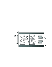
FIG. 1.: Field-induced director rotation in a conventional nematic (left) and nematic elastomer (middle) anchored at the surfaces $z=0$ and $z=d$, with an electric field $E$ applied across the cell. The shear strain $\lambda_{xz}$ accompanying the director rotation in nematic elastomers is shown on the right. The conventional Fredericks effect has one half wavelength of director rotation between the plates, while the solid nematic Fredericks effect has the full wavelength.

With all these preliminary restrictions and conditions, the full free energy density of the system takes the form:

$$f=\frac{1}{2}\mu\ {\sf Tr}\left[\underline{\underline{{\mathchoice{{\hbox{\boldmath$\displaystyle\ell$}}}{{\hbox{\boldmath$\textstyle\ell$}}}{{\hbox{\boldmath$\scriptstyle\ell$}}}{{\hbox{\boldmath$\scriptscriptstyle\ell$}}}}}}_{o}\cdot\underline{\underline{{\mathchoice{{\hbox{\boldmath$\displaystyle\lambda$}}}{{\hbox{\boldmath$\textstyle\lambda$}}}{{\hbox{\boldmath$\scriptstyle\lambda$}}}{{\hbox{\boldmath$\scriptscriptstyle\lambda$}}}}}}^{T}\cdot\underline{\underline{{\mathchoice{{\hbox{\boldmath$\displaystyle\ell$}}}{{\hbox{\boldmath$\textstyle\ell$}}}{{\hbox{\boldmath$\scriptstyle\ell$}}}{{\hbox{\boldmath$\scriptscriptstyle\ell$}}}}}}^{-1}\cdot\underline{\underline{{\mathchoice{{\hbox{\boldmath$\displaystyle\lambda$}}}{{\hbox{\boldmath$\textstyle\lambda$}}}{{\hbox{\boldmath$\scriptstyle\lambda$}}}{{\hbox{\boldmath$\scriptscriptstyle\lambda$}}}}}}\right]+\frac{1}{2}\mu\,A\,(\sin\theta-\lambda_{xz}\cos\theta)^{2}-\frac{1}{2}\varepsilon_{0}\Delta\varepsilon E^{2}\sin^{2}\theta+\frac{1}{2}K(\nabla{\rm\bf n})^{2}$$ (6)

The first term is the ideal nematic rubber elastic energy density [4] and can lead to the soft elastic response. The second term is the appropriate non-ideal, “semi-soft” contribution observed in many elastomers and, in particular, in those formed in a field-aligned monodomain state [10]. In elastomers $\mu$ gives the rubber energy scale, essentially a shear modulus at small deformations. The dimensionless parameter $A$ measures the (usually small) semi-softness. Inserting the deformation $\underline{\underline{{\mathchoice{{\hbox{\boldmath$\displaystyle\lambda$}}}{{\hbox{\boldmath$\textstyle\lambda$}}}{{\hbox{\boldmath$\scriptstyle\lambda$}}}{{\hbox{\boldmath$\scriptscriptstyle\lambda$}}}}}}$ and the director rotation $\theta$ (through $\underline{\underline{{\mathchoice{{\hbox{\boldmath$\displaystyle\ell$}}}{{\hbox{\boldmath$\textstyle\ell$}}}{{\hbox{\boldmath$\scriptstyle\ell$}}}{{\hbox{\boldmath$\scriptscriptstyle\ell$}}}}}}$), these two rubber-nematic terms take the form

$$f_{rub}=\frac{1}{2}\mu\,\left[\frac{(r-1)^{2}}{r}\sin^{2}\theta+\frac{r-1}{r}\,\sin 2\theta\,\lambda_{xz}+\frac{1+(r-1)\sin^{2}\theta}{r}\lambda_{xz}^{2}+A\,(\sin\theta-\lambda_{xz}\cos\theta)^{2}\right]$$ (7)

where we henceforth absorb the constant $3\mu/2$, the energy of the relaxed state, into $f$. The last two terms in equation (6) are conventional for liquid crystals. We adopt a simplified form of the dielectric term, with the field $E$ rather than the displacement $D$. The reasons for and the applicability of this simplification are discussed in the Appendix.

III Analysis of uniform director rotation

Without any assumptions of small deformations or angles, the optimal shear strain is given by the minimization of the free energy density $f_{rub}(\theta,\lambda)$, Eq. (7), with respect to $\lambda_{xz}$ at a given $\theta$. One obtains, after some straightforward algebra:

$$\lambda_{xz}(z) = -\frac{(r-A-1)\sin 2\theta}{2\left[1+Ar+(r-A-1)\sin^{2}\theta\right]},$$ (8)

where the local director rotation angle is, in fact, a function of $z$, $\theta=\theta(z)$. Substituting this back into the free energy density gives an effective free energy density, $f^{*}$, depending only on the ‘liquid crystal’ variable $\theta$.

$$f^{*}(\theta) = \frac{1}{2}\mu\,\left\{\frac{K}{\mu}(\nabla{\rm\bf n})^{2}-\frac{\varepsilon_{0}\Delta\varepsilon E^{2}}{\mu}\sin^{2}\theta+\right.$$ (10)

$$+\left.\bigg{[}\,\frac{(r-1)^{2}\sin^{4}\theta}{1+(r-1)\sin^{2}\theta}+\frac{A\,r^{2}\sin^{2}\theta}{(1+(r-1)\sin^{2}\theta)(1+A\,r+(r-A-1)\sin^{2}\theta)}\bigg{]}\right\}$$

The effect of the underlying rubbery network is expressed by the term in square brackets, $f^{*}_{rub}(\theta)$, an effective penalty for the uniform director rotation imposed by the elastic gel network. This expression is arranged in such a way that the contribution from the ideal soft nematic rubber elasticity is separated from the additional semi-soft part, the term proportional to the parameter $A$.

One can notice that at small deformations, $\theta\ll 1$, only the semi-soft correction contributes to the elastic energy, the first term in brackets being proportional to the higher power $\theta^{4}$ (appropriately expressing the softness of the ideal rubber-nematic response). Therefore, the main threshold for the uniform director rotation is determined by the semi-soft parameter $A$, which controls the counter-torque to the electric field. Note, that any effect of the field is scaled by the rubber modulus factor, yielding a reduced dimensionless electric field ${\cal E}=\left(\varepsilon_{0}\Delta\varepsilon E^{2}/\mu\right)^{1/2}$. In many cases this makes the response extremely small. However, the highly swollen network used in the experiments [6] (up to 90% solvent) may well have a much lower modulus (as will be indeed confirmed in Section VI). Also, as we shall see below, the scaling depends on the important polymer anisotropy $(r-1)$ too, so that the materials with small backbone chain anisotropy have, in fact, a stronger response to electric fields.

In spite of the obvious non-linearity of the effective free energy density (10), it is possible to solve exactly for the optimal director angle $\theta(E)$ by minimizing $f^{*}(\theta)$. The uniform, field-induced rotation of the director is

$$\sin^{2}\theta = -\frac{Ar+1}{r-Ar-1}+\frac{\sqrt{Ar+1}}{\sqrt{r-1-{\cal E}^{2}}\sqrt{r-Ar-1}}\ ;$$ (11)

$${\rm or}\ \ \ \theta^{2} \approx \frac{{\cal E}_{c}^{2}}{(r-1-{\cal E}_{c}^{2})^{2}}\left[{\cal E}/{\cal E}_{c}-1\right]\;,$$ (12)

where the second expression shows the variation of angle just above the bulk threshold. The appropriate reduced variable $x={\cal E}/{\cal E}_{c}-1$ is used near the threshold field, ${\cal E}_{c}$. The value of this threshold is:

$${\cal E}_{c}^{2}=\frac{Ar^{2}}{Ar+1}\;,$$ (13)

and is determined by both the semi-softness parameter (i.e. the director locking in the bulk) and the polymer chain anisotropy $r$. The solution Eq.(11) reaches its upper-bound at the field value

$${\cal E}_{u}^{2}=\frac{(r-1)^{2}(r+1)}{r^{2}}-A\frac{r-2-Ar}{r},$$ (14)

when $\sin\theta=1$ and the director rotation is complete. All this is in contrast with a conventional Fredericks effect, where there is no barrier for the uniform bulk director rotation and, if no boundary anchoring were involved, the director would switch to $\theta=\pi/2$ immediately at $E\neq 0$.

The conoscopy technique, used in experiments [6], reveals the change in optical path length for extraordinary rays traversing the sample $\delta=\frac{d}{\lambda}(n_{e}-n_{eff})$, with $d$ the cell thickness, and $\lambda$ the wavelength of light. The effective refractive index depends on the current director orientation $\theta(E)$ (we assume uniform rotation in this Section)

$$n_{eff}^{2}=\frac{n_{e}^{2}n_{o}^{2}}{n_{o}^{2}+(n_{e}^{2}-n_{o}^{2})\sin^{2}\theta}.$$ (15)

Near the threshold, when $\theta\ll 1$, the change in optical path is simply $\delta({\cal E})\approx\frac{d}{\lambda}\frac{n_{e}^{2}-n_{o}^{2}}{n_{o}^{2}}n_{e}\theta^{2}({\cal E})$. A plot of $\delta({\cal E})$ for $d/\lambda\sim 200$, $n_{e}=1.74,\ n_{o}=1.54$, very small semisoftness $A=0.001$ and increasing values of the chain anisotropy $r=1.1,\ 1.5$ and $2.5$ is given in Figure 2(a). Chains with higher anisotropy $r$ show a stronger resistance to an external torque, as one can see from equation (13). At fixed parameter $A$, the director response to the field is stronger when the chain anisotropy $r$ is reduced, as can be seen from the (expanded) equation (12). However the underlying resistance to rotation is because of the semi-soft, quadratic ($A$) terms in the rubber-nematic free energy, which is why the bulk threshold scales like ${\cal E}_{c}^{2}\sim A$. Only at larger rotations do the quartic terms (of order 1 rather than $A$) dominate, accounting for the scaling of the saturation field ${\cal E}_{u}^{2}$. Figure 2(b) shows the optical path $\delta({\cal E})$ at fixed chain anisotropy $r=1.5$ and increasing degree of network semi-softness, $A=0.001,\ 0.02,\ 0.05,\ 0.1$. At small angles $\delta\propto\theta^{2}$ and hence $\delta\sim({\cal E}-{\cal E}_{c})$ [see Eq.(12)]. Therefore increasing $A$ (and thus ${\cal E}_{c}$) increases the linear slope of the plots after the threshold, as seen in Figure 2 (b).

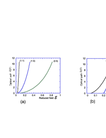
FIG. 2.: Change of extraordinary ray path length $\delta(\theta)$ versus electric field. (a) Small semi-softness $A=0.001$ with increasing chain anisotropy $r=1.1,1.5,2.5$ giving less rapid growth of $\delta$ with ${\cal E}$. (b) At fixed anisotropy $r=1.5$ with increasing $A=0.001,\ 0.02,\ 0.05,\ 0.1$ showing an increase in the threshold field ${\cal E}_{c}$ with increasing $A$.

Figure 3 uses the further reduced field $x={\cal E}/{\cal E}_{c}-1$, and the optical pathlength scaled by $(r-1-{\cal E}_{c}^{2})^{2}/{\cal E}_{c}^{2}$, as suggested by equation (12). Deviations from the initial linear response are evident for high threshold fields. From equation (11) for $\sin^{2}\theta$ we see there is a qualitative change in the field response for ${\cal E}_{c}^{2}=r-1$, that is where the semi-softness $A=(r-1)/r$. This condition is met either at low fields in networks of low anisotropy, $r-1$ small, or for fairly strong semi-softness, $A$ large. At ${\cal E}_{c}^{2}=r-1$ we have ${\cal E}_{u}^{2}={\cal E}_{c}^{2}$. There is no response to a field until it reaches ${\cal E}={\cal E}_{c}$, whereupon there is immediate, discontinuous switching $\theta\rightarrow\pi/2$.

Clearly, the existence of a threshold in field, rather than voltage, and quite a steep increase of the director rotation [and consequently of the observed optical path $\delta({\cal E})$] are described well. However, there are two important aspects still missing: (1) the analysis of boundary conditions and non-uniform deformations, which leads to a Fredericks threshold voltage in conventional nematics, and (2) the experimentally observed small increase in rotation before the principal threshold, a “precursor foot” which we shall associate with a small degree of random misorientation in the initial director distribution.

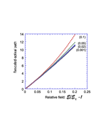
FIG. 3.: The conoscopic response for the conditions of figure 2(b). The field is further reduced to $x={\cal E}/{\cal E}_{c}-1$, and optical pathlength is scaled by $(r-1-{\cal E}_{c}^{2})^{2}/{\cal E}_{c}^{2}$, which collapses the plots of Fig. 2b for various $A$ onto the single curve, Eq.(12), in the region of the transition, $x\ll 1$.

IV Critical analysis of the transition region

The analysis of the previous Section assumes that there is no relevant spatial variation in either $\theta(z)$, or $\lambda_{xz}(z)$: the solution for $\theta(E)$, equations (11) and (12), has been obtained without taking into account the director-gradient Frank elasticity. This is a reasonable assumption at fields high above the threshold, where the texture is coarsened and the bulk is capable of achieving its optimal value of $\theta$, equation (11), which we shall call $\theta_{0}$ (similarly, for the conventional Fredericks effect $\theta_{0}\rightarrow\pi/2$ and the profile $\theta(z)$ coarsens at high fields). Near the threshold one has to be more careful and examine the effect of boundary conditions (which is the only existing barrier for the conventional Fredericks effect).

Near the threshold we can safely assume $\theta\ll 1$ and the free energy density takes the form, standard for elliptic-function analysis (see Appendix)

$$\frac{1}{\mu}f^{*}\approx\frac{1}{2}(\theta^{\prime})^{2}-\frac{1}{2}p\,\theta^{2}+\frac{1}{4}q\,\theta^{4},$$ (16)

with the coordinate $z$ scaled by the natural length scale $\xi=\sqrt{K/\mu}$. For a typical rubber modulus, as in experiments [10], $\xi\sim 10^{-8}\hbox{m}$. Parameters $p$ and $q$ are obtained by expanding the full free energy density (10):

$$p = {\cal E}^{2}-\frac{A\,r^{2}}{1+Ar},$$ (17)

$$q \approx 2\left[(r-1)^{2}-\frac{Ar^{2}}{1+Ar}\left(r-1+\frac{r-1-A}{1+Ar}\right)\right].$$ (18)

In $q$ we have put ${\cal E}^{2}\sim Ar^{2}/(1+Ar)$; that is we are close to the threshold, and have neglected other terms discussed in the Appendix. The details of this type of analysis are also given in the Appendix of paper [10]: the director cannot achieve its local optimal orientation $\theta_{0}=\sqrt{p/q}$, being held by boundary conditions. Instead, the director is only having a modulation of amplitude $\theta_{m}$ ($<\theta_{0}$) across the cell. The resulting “order parameter” $\eta(E)=\theta_{m}/\theta_{0}$ increases from zero towards 1 as the texture coarsens. The number of periods of the elliptic function that describes the variation $\theta(z)$ is $\frac{d}{4\sqrt{2}\xi{\sf K}}\sqrt{p(2-\eta^{2}})$ with ${\sf K}$ the complete elliptic integral of argument $\eta^{2}/(2-\eta^{2})$. The minimal number of periods in our case is one (in contrast with the usual symmetric Fredericks effect, where it is a half), so one obtains the director rotation angle $\theta_{m}$ as the solution $\eta(E)$ of

$$\frac{1}{\sqrt{2-\eta^{2}}}{\sf K}[\eta] = \frac{d\sqrt{p}}{4\sqrt{2}\xi}$$ (19)

$$\equiv \frac{1}{4\sqrt{2}}\frac{d}{\sqrt{K}}\sqrt{\varepsilon_{0}\Delta\varepsilon E^{2}-\mu\frac{Ar^{2}}{1+Ar}}\qquad\ \ \left(\Rightarrow\frac{1}{2\sqrt{2}}\sqrt{\frac{\varepsilon_{0}\Delta\varepsilon}{K}}E\,d\right)\;.$$ (20)

The expression in parentheses is the corresponding right-hand side for the conventional Fredericks effect, with no underlying rubber elasticity $\mu$ and $A=0$ (and with the half- rather than full-period of director oscillation across the cell thickness); it depends on a voltage $V=E\,d$. The real threshold is shifted from that of the uniform analysis of last Section, equation (13), by the additional contribution from the domain walls (which is the only contribution in the conventional Fredericks effect): the solution of (19) first appears at the minimal value of ${\sf K}=\pi/2$ at $\eta=0$, i.e. $p^{*}=(2\pi\xi/d)^{2}$:

$$E^{*}\approx\sqrt{\left(\frac{\mu}{\varepsilon_{0}\Delta\varepsilon}\right)\frac{A\,r^{2}}{1+Ar}+\left(\frac{2\pi}{d}\right)^{2}\frac{K}{\varepsilon_{0}\Delta\varepsilon}}\qquad\left[{\rm normally\ we\ expect\ \ }\frac{A\mu d^{2}}{K}\gg 1\ \right]\;.$$ (21)

One should note that the analysis of the threshold itself is elementary and does not require the investigation of the elliptic function. In the usual way, we could introduce a variation of wave vector $k$ $(=2\pi/d)$ whereupon the expanded free energy density (16) is $f\sim\frac{1}{2}(k^{2}-p)\theta^{2}+\frac{1}{4}q\theta^{4}$. Modulation starts when the $\theta^{2}$-coefficient becomes negative for the first time, whence the threshold condition (21) is recovered.

Returning to the elliptic analysis, near the threshold the director rotation is given by $\eta^{2}=\frac{4}{3}(p-p^{*})/p^{*}$, describing the full-wavelength modulation with the amplitude $\theta_{m}=\eta(E)\theta_{0}(E)$. The effect of this elliptic analysis near the threshold rapidly disappears as the modulation coarsens, the optimal value $\theta_{0}$ of the director rotation being achieved in most of the sample and the $\delta(E)$ variation becoming that of equation (15).

We said that one normally expects $(\mu d^{2}/K)\gg 1$, the thickness-dependent term thus being irrelevant in the expression for the threshold. As discussed below, effects observed in thin samples suggest that the effective rubber modulus, $\mu A$, is low in the studied material. Although this may in part be because $\mu$ is small due to dilution by solvent, it clearly indicates that $A$ is small too. If the effect were simply due to the smallness of $\mu$ alone, then the quartic terms would also be weakened and the saturation field ${\cal E}_{u}$ would also be accessible. Because $A$ is evidently small, it may be possible to see the remaining $d$-dependence of the apparent threshold in experiment and compare it with (21).

V Oblique initial director

There seems to be no reason to assume a systematic obliqueness (pre-tilt) in the initial director. However, the preparation of networks, especially in thick cells, results in a residual polydomain texture, as reported by Chang et al. and is a well-established phenomenon in nematic gels. Even after orientation by strong magnetic fields one should expect a small degree of remaining random disorder, see [11]. Assuming the degree of this misalignment is small, it is straightforward to make provisions for it and obtain the resulting quenched averages of observable parameters, such as the director angle $\theta({\cal E})$ and the optical path $\delta({\cal E})$.

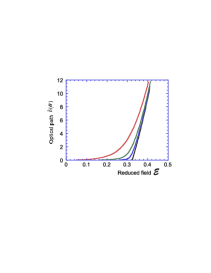
FIG. 4.: Conoscopic path length $\delta$ vs. reduced electric field for backbone chain anisotropy $r=1.5$, semi-softness parameter $A=0.05$ and increasing r.m.s. misalignment angle $\alpha=0,\ 0.01,\ 0.03,\ 0.05,\ 0.1$ radians.

We do not go into details of this calculation, which involves some heavy algebra. Instead, we plot the results for several values of parameters. The plots in Figure 4 show the optical path $\delta({\cal E})$ for selected values $r=1.5,\ A=0.05$ and increasing r.m.s. misalignment $\alpha=0,\ 0.01,\ 0.03,\ 0.05,\ 0.1$ (the last value corresponds to $\alpha=5.7$ deg). The misalignment not only creates a precursor foot before the main threshold, but also changes the slope so that the extrapolated value of ${\cal E}$ appears slightly reduced from $E^{*}$ in (21). We emphasize that theory and physical expectations suggest the obliqueness $\alpha$ should strongly depend on cell thickness and on the magnetic field used during crosslinking.

VI Experimental observations

We now apply the model of the previous sections to the experimental observations of Chang et al. [6], in light of further experiments performed recently. The analysis of data performed by Chang et al. includes a bulk anchoring effect similar to that proposed here, which produces a threshold field, rather than voltage. However, they also appealed to an intrinsic material length scale on the order of micrometers, which further increases the observed threshold field and also sets the scale for director gradients, which limit the director rotation above threshold. They reported observations of micrometer scale speckles in the sample after polymerization in support of this proposed length scale, but did not directly observe a periodic pattern of director rotation at the micrometer scale in response to the applied electric field.

We prepared a series of samples of different thicknesses according the the methods of Chang et al., and performed microscopic observations during application of the field. In thick samples, comparable to those of [6], we observed the same general elements of response that they reported, but in addition, we were able to observe small scale movements in the sample, particularly displacements of microscopic particles and speckles in the sample. We observed lateral displacements in the plane of the sample on the order of a fraction of the sample thickness, and saw no evidence of micrometer scale deformations in response to the field. Our observations are consistent with the deformation sketched on the right in figure 1, which involves a combination of shear strains resulting in lateral displacement of material in the midplane of the sample. The deformation proposed on the right in Fig. 1 also satisfies the preservation of symmetry in the conoscopic image reported by Chang et al., in contrast to the rotation of the optical axis that would accompany the classical half-wavelength Fredericks transition. Thus, the field response proposed here is completely consistent with the general observations reported by Chang et al. [6]. Moreover, as described in the previous Section, the pretransitional response, or rounding of the transition, observed by Chang et al. can be similarly explained by a small random pre-tilt of the director.

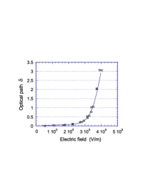
FIG. 5.: Theoretical curve of $\delta(E)$, the conoscopic length, against electric field for the present theory (solid line) for thick samples (uniform director rotation) to the data of Chang et al. [6]. For the 62 $\mu$m thick sample (crosses) we have doubled the data values for the optical pathlength $\delta$ to collapse the data from two samples onto the same plot. For the 125 $\mu$m thick sample (squares) the data are unscaled. This is the same scaling used in Fig. 1 of [6].

Taking the published data of Chang et al., and using the model of Section III appropriate for thick samples, along with pretilt of the director, we present a fit of the present theory to the data in figure 5. We plot our theoretical prediction of $\delta$ using $\theta$ from 11 and taking the values $r$ = 1.95, $A$ = 0.06, $\mu=1.6\times 10^{2}$ J/m³, and $\alpha$ = 1.7 degrees for the network, in addition to the sample characteristics specified by Chang et al.. We see that this theory can reproduce the experimental observations with reasonable values of sample thickness etc. [13]. The values of semi-softness parameter $A$ and of the random local pretilt angle $\alpha$ are sufficiently small not to contradict the known facts about liquid crystalline gels. The value of backbone anisotropy $r$, slightly higher than that reported for solvent free polyacrylate elastomers ($\sim$ 1.44 [9, 14]), is likely due to the large amount of nematic solvent present in the gel and increasing the nematic field. The solvent (up to 90%) can also explain the very small value of rubber modulus $\mu$. In fact, it is mostly due to this weakness of swollen elastic network that we can observe a noticeable director rotation, the angle of which depends on a ratio $E\left(\varepsilon_{o}\Delta\varepsilon/\mu\right)^{1/2}$. However, in spite of this plausibility, independent measurements of these parameters are needed to test the presented theory more explicitly.

The value of the gel modulus $\mu$, used in the fitting above, is substantially lower than that expected for ordinary rubbers. It necessitates re-examination of the characteristic length scales in our system. The natural nematic elastomer scale $\xi=\sqrt{K/\mu}$ (see Eq.(16) and, more comprehensively, the review [4]) is now of the order $10^{-6}$m. This scale gives the characteristic thickness of domain walls, two of which are present in the full-wavelength Fredericks geometry, Fig. 1. Hence one expects that thin samples, with $d$ only of order of several micrometers, should deviate from the description proposed here: In thick samples, our electro-mechanical response is driven by a reduction in electrical energy because of director rotation toward the field with very little elastic penalty, since the deformations are soft in the uniform regions above and below the midplane. These regions are separated by a domain wall in the middle, where the shear strain reverses sign. When the sample thickness is reduced, this wall and the two non-uniform regions near the cell boundaries would start merging. This raises the elastic energy of the full-wavelength (nematic elastomer-like) Frederiks transition above that of the half-wavelength (liquid nematic-like) one. Indeed, in thin samples (8 to 25 micrometers in thickness), we observed the different response, almost identical to the ordinary half-wavelength Fredericks transition. This was evident in the conoscopic observations, by the rotation of the optical axis in response to the applied field, as in low-molar mass nematic liquid crystals.

To satisfy the boundary conditions with this fully non-uniform director rotation, the predominant shear strain in the bulk of the sample must be zero. The energy penalty and the counter-torque for the action of electric field are then provided by Eq.(7) with $\lambda_{xz}=0$. This is the regime of “couples without strains”, with a bulk barrier for the director rotation, first proposed by de Gennes [15]. More detailed experimental measurements and theoretical analysis will be carried out to explore this kind of transition in thin samples, and to determine the thickness at which the crossover from thin to thick behavior occurs. This will provide a detailed understanding of the combined director and shear strain structure within the boundary layers and give an independent measure of the effective rubber modulus $\mu$ via the characteristic length scale $\xi$.

Another aspect that needs to be re-examined for a system with very low modulus $\mu$ is the threshold condition, Eq.(21). In order to predict the field threshold $E^{*}$, rather than the voltage $V^{*}=E.d$, we need to maintain the inequality $A\mu d^{2}/K\gg 1$. For the values used in fitting the experimental data in Fig.5 (for the smaller $d\simeq 60\,\mu\hbox{m}$) we still obtain a ratio of order $3\times 10^{3}$ and the conclusions about the threshold remain valid. However, this ratio will become of order unity for $d\sim 10^{-6}$ m, where the ordinary voltage threshold should again become relevant.

VII Conclusion

In summary, we propose a model for the Fredericks transition in nematic polymer gels. Especially for thick samples, the polymer network serves both to set the threshold field for the transition, and to control the director response above threshold. It effectively replaces the role of the sample surfaces in the ordinary nematic Fredericks transition. We can reasonably explain the experimental results of Chang et al. without appealing to a new internal length scale for director gradients, and this element of our explanation is supported by qualitative experimental observations of macroscopic lateral displacements in response to the applied field.

Because two coupled physical fields, the director angle $\theta$ and the shear strain $\lambda_{xz}$, are at play, it is possible that there are two different characteristic timescales for relaxation. Depending upon the disparity of these, one could at short timescales possibly see another decay regime before the final, slowest exponential decay reported by Chang et al.. This obtains naturally from the numerical solution of the dynamical equations in $\theta$ and $\lambda_{xz}$ resulting from Eq.(6) (see [16]).

We have begun to examine the remaining role of director and shear strain gradients in the sample, and our experimental observations suggest that this is important for understanding the transition in thin samples. Much experimental work remains to be done to test various aspects of our model. Finally, it is interesting to compare these predictions for nematic gels with the behavior of polymer-stabilized liquid crystals. The key difference is the permanently fixed macroscopic polymer skeleton of the PSLC system, in contrast with the mobile molecular scale network of a gel. The detailed analysis of the threshold, director evolution at higher fields and the role of alignment conditions at preparation should distinguish between the behavior of these two systems. The dynamic behavior is especially different, with gels responding very slowly, compared to PSLC’s.

ACKNOWLEDGEMENTS

This research was supported in part by the National Science Foundation through grant DMR-9415656 at Brandeis university, and by EPSRC in the UK.

A Analysis of dielectric problem

In the classical electric Fredericks problem the anisotropic dielectric fluid is contained between two parallel plates kept at a relative voltage $V$ [12]. The analysis can easily be generalized to the elastic-electric case. One needs to use the electric displacement vector ${\rm\bf D}=(0,0,D)$, which is a constant between the plates given no space charge ($div\,{\rm\bf D}=0$). The field $E$ and the displacement $D$ are related by ${\rm\bf D}=\varepsilon_{o}\underline{\underline{\varepsilon}}\cdot{\rm\bf E}$. As all nematic uniaxial tensors, the matrix of dielectric constants is expressed as $\varepsilon_{ij}=\varepsilon_{\bot}\delta_{ij}+(\varepsilon_{\parallel}-\varepsilon_{\bot})n_{i}n_{j}$, where the nematic director n is the principal axis. The voltage is, therefore, given by the integration $\int E_{z}dz$:

$$V=\int_{0}^{d}dz\frac{D}{\varepsilon_{o}(\varepsilon_{\bot}+\Delta\varepsilon\sin^{2}\theta)},$$ (A1)

where $\varepsilon_{zz}=\varepsilon_{\bot}+\Delta\varepsilon\sin^{2}\theta$. The correct free energy, now per unit area of plates, does not derive from equation (6), but from the dielectric energy density $-({\rm\bf D}\cdot{\rm\bf E})$:

$$F = \int_{0}^{d}dz\left[\frac{1}{2}K\left(\frac{d\theta}{dz}\right)^{2}+\mu g(s)-\frac{1}{2\varepsilon_{o}}D^{2}\frac{1}{\epsilon_{\bot}+\Delta\epsilon\sin^{2}\theta}\right]$$ (A2)

$$\equiv \int_{0}^{d}dz\left[\frac{1}{2}K\left(\frac{d\theta}{dz}\right)^{2}+\mu g(s)\right]\ -\ \frac{\varepsilon_{o}V^{2}}{2}\frac{1}{\int_{0}^{d}\frac{dz}{\varepsilon_{\bot}+\Delta\varepsilon\sin^{2}\theta}}\ ,$$ (A3)

where $\mu g(s)$ is the rubber-nematic part of free energy density, given by equation (7). The Euler-Lagrange equation giving the $\theta(z)$ minimizing this free energy is:

$$K\theta^{\prime\prime}=\mu\frac{dg}{d\theta}+\left(\frac{D^{2}}{2\varepsilon_{o}}\right)\,\frac{d}{d\theta}\left(\frac{1}{\varepsilon_{\bot}+\Delta\varepsilon\sin^{2}\theta}\right)$$ (A4)

where the constant $D$ has to be determined from equation (A1) and is thus a functional of $\theta(z)$. The boundary conditions are $\theta^{\prime}=0$ at $\theta=\theta_{m}$ if there is a modulation with amplitude $\theta_{m}$. Then Eq. (A4) is easily integrated once to give:

$$\left(\frac{d\theta}{du}\right)^{2}=2\left(g(\sin^{2}\theta)-g(\sin^{2}\theta_{m})\right)+\frac{D^{2}}{\mu\varepsilon_{o}}\left(\frac{1}{\varepsilon_{\bot}+\Delta\varepsilon\sin^{2}\theta}-\frac{1}{\varepsilon_{\bot}+\Delta\varepsilon\sin^{2}\theta_{m}}\right)\;,$$ (A5)

where $u=z/\xi$ is the length reduced by the rubber-nematic correlation length $\xi=\sqrt{K/\mu}$. The full problem is solved by further integrating over 1/4 period and yields:

$$\int_{0}^{\theta_{m}}\frac{d\theta}{\left[\dots\right]}=\frac{d}{4\xi}$$ (A6)

where $\left[\dots\right]$ is the right hand side of Eq. (A5). The right hand side of Eq. (A6) is a quarter period of the modulation. Integrating Eq (A5) to a general $\theta$ at a general $z$, rather than to $\theta_{m}$ and $d/4$ as in Eq. (A6), gives $\theta(z)$ as an elliptic function, which then finally determines $D$ via Eq. (A1) and thereby in Eq. (A6) itself.

At the vicinity of the transition, all this analysis significantly simplifies since $\sin^{2}\theta\leq\sin^{2}\theta_{m}\leq\sin^{2}\theta_{o}\ll 1$. $D$ and $V$ are trivially related as $D=\varepsilon_{o}\varepsilon_{\bot}V/d$. The potential $g(s)+\frac{D^{2}}{\varepsilon_{o}}\frac{1}{\varepsilon_{\bot}+\Delta\varepsilon\sin^{2}\theta}$ driving Eq. (A5) simplifies to $-\frac{1}{2}p\theta^{2}+\frac{1}{4}q\theta^{4}$ with $p$ and $q$ given in the equation (17). The elliptic analysis then follows as if from the simplified free energy Eq. (6).

In the uniform case considered in Section III the distinction between $D$ and $E$ is easily handled too since Eq. (A1) collapses to the obvious $D=\varepsilon_{o}({\varepsilon_{\bot}+\Delta\varepsilon\sin^{2}\theta})V/d$ and the electrical part of equation (A2) gives the $\theta$-dependent part of the electrical energy in equation (10) (a constant part having been suppressed).

REFERENCES

- [1] L. Golubovic and T.C. Lubensky, Phys. Rev. Letters 63, 1082 (1989).
- [2] M. Warner, E.M. Terentjev and P. Bladon, J. Physique II 4, 93 (1994).
- [3] J. Kupfer and H. Finkelmann, Macromol. Chem. Phys. 195, 1353 (1994).
- [4] M. Warner and E.M. Terentjev, Progr. Polym. Sci. 21, 853 (1996).
- [5] R. Zentel, Liq. Cryst. 1, 589 (1986); N.R. Barnes, F.J. Davis and G.R. Mitchell, Mol. Cryst. Liq. Cryst. 168, 13 (1989); R. Kishi, Y. Suzuki, H. Ichijo and O. Hirasa, Chem. Lett. 12, 2257 (1994).
- [6] C.-C. Chang, L.-C. Chien and R.B. Meyer, Phys. Rev. E56, 595 (1997).
- [7] D.K Yang, L-C. Chien and J.W. Doanne, Appl. Phys. Lett. 60, 3102 (1992).
- [8] R.J. Atkins and N. Fox, An Introduction to the Theory of Elasticity, Longman, London, 1980.
- [9] G.R. Mitchell, F.J. Davis, W. Guo and R. Cywinski, Polymer 32, 1347 (1991).
- [10] H. Finkelmann, I. Kundler, E.M. Terentjev and M. Warner, J. Physique I 7, 1059 (1997).
- [11] S.V. Fridrikh and E.M. Terentjev, Phys. Rev. Letters 79, 4661 (1997).
- [12] W.H. de Jeu, Physical Properties of Liquid Crystals, Gordon and Breach, NY, 1980.
- [13] The data in figure 1 of the paper by Chang et al. [6], and the theoretical curves fitting the data are scaled differently for the two samples they examined. This is not fully explained in their figure caption, but is referred to in their text. They double the data for the change of extraordinary ray optical pathlength for the 62 m sample, while not rescaling the voltage data.
- [14] E.R. Zubarev, R.V. Talroze, T.I. Yuranova, N.A. Plate and H. Finkelmann, Macromolecules 31, 3566 (1998).
- [15] P.G. de Gennes, C.R. Acad. Sci. B281, 101 (1975).
- [16] P.I.C. Teixeira, European Phys. J. B, submitted, 1998.