Multiple Andreev reflections as a transport problem
in energy space

Abstract

We present an approach for analyzing the dc current in voltage biased quantum superconducting junctions. By separating terms from different $n$-particle processes, we find that the $n$-particle current can be mapped on the problem of wave transport through a potential structure with $n$ barriers. We discuss the relation between resonances in such structures and the subgap structures in the current-voltage characteristics. At zero temperature we find, exactly, that only processes creating real excitations contribute to the current. Our results are valid for a general SXS-junction, where the X-region is an arbitrary non-superconducting region described by an energy-dependent transfer matrix.

(Submitted 12 November 1998)

1 Introduction

Multiple Andreev reflection (MAR), first suggested by Klapwijk, Blonder, and Tinkham [1] for explaning the subharmonic gap structure (SGS) in SNS junctions, is presently accepted as a general mechanism of subgap current transport in superconducting junctions. During the last five years a considerable effort has gone into developing a consistent theory of MAR capable of including effects of quantum coherence and normal electron scattering by the junction. Different techniques have been used for calculating current-voltage characteristics, including various modifications of Keldysh formalism [2, 3, 4, 5] and the Landauer-Büttiker scattering method [6, 7, 8, 9, 10, 11]. The theory has been extended to resonant tunnel junctions [12, 13, 14, 15] and junctions of d-wave superconductors [16]. The theory has successfully explained the SGS in transmissive planar junctions [17] and atomic-size point contacts [18]. The good agreement between the theory and experimental data obtained for one-channel tunnel junctions without fitting parameters [19] has provided a firm basis for further investigations - revealing the transport channels and transmissivity of individual channels in single-atom contacts [20, 21].

Despite successful numerical calculations of subgap current- voltage characteristics for different types of junctions, the general understanding of MAR is still not sufficient, and interpretation of particular features of SGS, e.g. current peaks, presents difficulties. This especially concerns resonant MAR, where the energy dispersion of electron scattering phase shifts is important.

In this paper, we present an approach where MAR is treated as a wave propagation problem in energy space (cf. [9]). Using scattering theory formalism, we derive an adequate mapping of MAR onto a transmission problem through a 1D wave guide with a built in multiple tunnel barrier structure. All parameters of this structure are uniquely determined by the junction characteristics (normal and Andreev scattering amplitudes) and by the applied voltage. In terms of such a mapping, the onsets and peaks of SGS are explained in terms of resonances in the transmission along the energy axis. The mapping allows us consistently to separate currents associated with $n$-particle transmission processes [22] and to prove the cancellation of non-physical ground state currents, which is equivalent to the Pauli exclusion principle.

2 Model and ansatz

We consider two superconducting reservoirs connected to a single normal conducting channel which may contain tunnel barriers (X-region) (see Fig. 1). The transport properties of this channel is described by its transfer matrix. Using an energy dependent transfer matrix we can model any effective single-particle potential structure, including the important scattering phase shifts in long and resonant junctions. In general the transfer matrix is also voltage dependent, and deriving this dependence for any given physical model is a problem in its own right. But having found this transfer matrix, we can determine the current when the contacting reservoirs are in the superconducting state.

We place the origin of our coordinate system in the middle of the junction; the normal-superconducting (NS) interfaces are then located at $-L/2$ and $L/2$, where $L$ is the length of the junction (Fig. 1). Due to the point-contact geometry of our junction, the superconducting pair potential can be considered steplike, $\Delta(x)=\Delta_{0}\Theta(|x|-L/2)$.

We will construct scattering states in terms of the transfer matrix of the X-region. To this end we introduce two auxilliary normal regions, between the X-region and the superconducting electrodes. These regions are assumed to have the same material parameters as the electrodes, providing perfect NS-interfaces, and their length is much smaller than the coherence length.

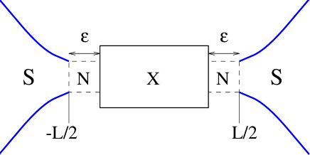
Fig.  1: Sketch of the junction geometry: The junction consists of an arbitrary normally conducting, single channel region (X), connected to two superconducting reservoirs (S). Two ballistic normal regions (N) of length $\epsilon$ between the X and S regions are introduced for convenience. $\epsilon$ is much smaller than the coherence length.

To calculate the scattering states we first make an ansatz in terms of a sum of plane-wave solutions to the Bogoliubov-de Gennes (BdG) equation in the left/right auxiliary normal regions ($\Psi_{LN}/\Psi_{RN}$) and in the left/right superconductors ($\Psi_{LS}/\Psi_{RS}$). In superconductors, the energy is commonly counted from the chemical potential which is motivated by the electron-hole symmetry. This is not convenient in voltage biased junctions because the chemical potentials in the left ($\mu_{LS}$) and right ($\mu_{RS}$) electrodes are different. A global reference of energy, which is particularly desirable in the case of an energy dependent transfer matrix, can be introduced by making different gauge transformations in the left and right superconducting electrodes. This procedure gives rise to the appearance of time-dependent phase factors in the wave functions of the superconducting electrodes implying inelastic scattering. To get symmetrical expressions for quasiparticles incoming from the left and from the right we choose $(\mu_{LS}+\mu_{RS})/2$ as a global reference of energy, i.e. the reference energy is in the middle of the chemical potentials in the left and right superconductors. We thus get different time-dependences for electron and hole components in both superconductors,

$$\Psi_{LN} = \sum_{n=\bar{\infty}}^{\infty}\left(\begin{array}[]{c}\alpha_{n}e^{ik^{e}_{n}(x+L/2)}+\beta_{n}e^{-ik^{e}_{n}(x+L/2)}\\ \gamma_{n}e^{ik^{h}_{n}(x+L/2)}+\delta_{n}e^{-ik^{h}_{n}(x+L/2)}\end{array}\right)e^{-i(E_{n}+eV/2)t},$$ (3)

$$\Psi_{RN} = \sum_{n=\bar{\infty}}^{\infty}\left(\begin{array}[]{c}\alpha_{n}^{\prime}e^{ik^{e}_{n}(x-L/2)}+\beta_{n}^{\prime}e^{-ik^{e}_{n}(x-L/2)}\\ \gamma_{n}^{\prime}e^{ik^{h}_{n}(x-L/2)}+\delta_{n}^{\prime}e^{-ik^{h}_{n}(x-L/2)}\end{array}\right)e^{-i(E_{n}+eV/2)t},$$ (6)

$$\Psi_{LS} = e^{-i\sigma_{z}eV/2t}\cdot\left[\left(\delta_{1\sigma}\hat{u}^{e}_{n}e^{+i\tilde{k}^{e}_{0}(x+L/2)}+\delta_{2\sigma}\hat{u}_{n}^{h}e^{-i\tilde{k}^{h}_{0}(x+L/2)}\right)e^{-iEt}+\right.$$ (7)

$$+ \left.\sum_{n=\bar{\infty}}^{\infty}\left(A_{n}\hat{u}_{n}^{e}e^{-i\tilde{k}^{e}_{n}(x+L/2)}+B_{n}\hat{u}_{n}^{h}e^{+i\tilde{k}^{h}_{n}(x+L/2)}\right)e^{-iE_{n}t}\right],$$

$$\Psi_{RS} = e^{i\sigma_{z}eV/2t}\cdot\left[\left(\delta_{3\sigma}\hat{u}_{n}^{e}e^{-i\tilde{k}^{e}_{0}(x-L/2)}+\delta_{4\sigma}\hat{u}_{n}^{h}e^{+i\tilde{k}^{h}_{0}(x-L/2)}\right)e^{-iEt}+\right.$$ (8)

$$+ \left.\sum_{n=\bar{\infty}}^{\infty}\left(C_{n}\hat{u}_{n}^{e}e^{i\tilde{k}^{e}_{n}(x-L/2)}+F_{n}\hat{u}_{n}^{h}e^{-i\tilde{k}^{h}_{n}(x-L/2)}\right)e^{-iE_{n}t}\right].$$

In the ansatz in Eqs. (3)-(8), $E$ denotes the energy of the incoming particle, $E_{n}=E+neV$, and the index $\sigma\in\{1,2,3,4\}$ denotes the incoming quasiparticles $\{e^{\rightarrow},h^{\rightarrow},e^{\leftarrow},h^{\leftarrow}\}$ respectively. $\hat{u}_{n}^{e}=(u_{n},v_{n})$ and $\hat{u}_{n}^{h}=(v_{n},u_{n})$ are vectors describing bulk electron- and hole-like quasiparticles respectively.

By matching the wave functions across the NS intefaces we get the boundary conditions for the wave function in the normal region, including the source term. By defining coefficient vectors $\hat{\alpha}_{n}=(\alpha_{n},\beta_{n})$ and $\hat{\gamma}_{n}=(\gamma_{n},\delta_{n})$, and similar for the primed quantities in Eq. (6), we may write these boundary conditions in the following form,

$$\hat{\alpha}_{n}={\bf U}_{n}\hat{\gamma}_{n-1}+\delta_{n0}(u_{0}^{2}-v_{0}^{2})\left(\begin{array}[]{c}\delta_{1\sigma}/u_{0}\\ -\delta_{2\sigma}/v_{0}\end{array}\right),\hskip 14.22636pt\hat{\gamma}^{\prime}_{n}={\bf U}_{n}\hat{\alpha}^{\prime}_{n-1}+\delta_{n0}(u_{0}^{2}-v_{0}^{2})\left(\begin{array}[]{c}\delta_{4\sigma}/u_{0}\\ -\delta_{3\sigma}/v_{0}\end{array}\right),$$ (9)

where ${\bf U}_{n}=diag(a_{n},a_{n}^{-1})$ is the Andreev reflection matrix and $a_{n}$ is the amplitude of Andreev reflection,

$$a_{n}=\frac{v_{n}}{u_{n}}=\left\{\begin{array}[]{cc}\left(E_{n}-\mbox{sign}(E_{n})\sqrt{E_{n}^{2}-\Delta^{2}}\right)/\Delta&|E|>\Delta\\ \left(E_{n}-i\sqrt{\Delta^{2}-E_{n}^{2}}\right)/\Delta&|E|<\Delta\end{array}\right..$$ (10)

In this derivation we have neglected the difference in wave vectors between the normal and superconducting regions (quasiclassical approximation). The coefficients in Eqs. (3)-(6) are connected by the transfer matrix ${\bf T}(E)$ describing the X-region,

$$\hat{\alpha}_{n}={\bf T}(E_{n}+eV/2)\hat{\alpha}^{\prime}_{n}\hskip 28.45274pt\hat{\gamma}_{n}={\bf T}(-(E_{n}+eV/2))\hat{\gamma}^{\prime}_{n}.$$ (11)

Equations (9)-(11), together with the boundary condition of vanishing coefficients for $|n|\rightarrow\infty$, completely determine the scattering states.

Checking equations (9)-(11) one may find that in any scattering state half of the coefficients in the ansatz will be zero. For example, for $\sigma\in\{1,2\}$ the nonzero coefficients will be $\hat{\alpha}_{2m}$ and $\hat{\gamma}_{2m-1}$, while for $\sigma\in\{3,4\}$ $\hat{\alpha}_{2m-1}$ and $\hat{\gamma}_{2m}$ will be nonzero. To get rid of the redundant coefficients we define new coefficients $c_{n\pm}$. For $\sigma\in\{1,2\}$ the definition reads $\hat{c}_{2m+}=\hat{\alpha}_{2m}$, $\hat{c}_{2m-}=\hat{\gamma}_{2m-1}$, $\hat{c}_{(2m+1)+}=\hat{\gamma}^{\prime}_{2m+1}$ and $\hat{c}_{(2m+1)-}=\hat{\alpha}^{\prime}_{2m}$. These coefficients are connected by transfer matrices ${\bf T}^{l}_{n}$ with even indices ${\bf T}^{l}_{2m}=\left[{\bf T}(E_{2m}+eV/2)\right]^{-1}$ and odd indices ${\bf T}^{l}_{2m-1}={\bf T}(-(E_{2m-1}+eV/2))$. For the purpose of treating quasiparticles incoming from the left and right on an equal footing we introduce similar notations for $\sigma\in\{3,4\}$: $\hat{c}_{2m+}=\hat{\gamma}^{\prime}_{2m}$, $\hat{c}_{2m-}=\hat{\alpha}^{\prime}_{2m-1}$, $\hat{c}_{(2m+1)+}=\hat{\alpha}_{2m+1}$ and $\hat{c}_{(2m+1)-}=\hat{\gamma}_{2m}$ and matrices ${\bf T}^{r}_{2m}={\bf T}(-(E_{2m}+eV/2))$ and ${\bf T}^{r}_{2m-1}=\left[{\bf T}(E_{2m-1}+eV/2)\right]^{-1}$.

Using these definitions the equations (9)-(11) can, for quasiparticles incoming from both left and right, be written as:

$$\hat{c}_{n+}={\bf U}_{n}\hat{c}_{n-}+\delta_{n0}(u_{0}^{2}-v_{0}^{2})\left(\begin{array}[]{c}(\delta_{1\sigma}+\delta_{4\sigma})/u_{0}\\ -(\delta_{2\sigma}+\delta_{3\sigma})/v_{0}\end{array}\right),\hskip 28.45274pt\hat{c}_{(n+1)-}={\bf T}_{n}\hat{c}_{n+}.$$ (12)

Note that even though these equations are formally identical for quasiparticles incoming from both left and right, the ${\bf T}_{n}$-matrices involved in the two cases are different. In Figure 2a we show the structure of Eqs. (12) for an electron-like quasiparticle incoming from the left.

Fig.  2: Schematic structure of a scattering state (a) and its probability currents (b). Figure (a) shows schematically the connection between different coefficients and transfer matrices for an electronlike quasiparticles incoming from the left ($\sigma=1$). Figure (b) shows schematically how the probability current from the incoming quasiparticle enters the normal region and divides into upgoing ($j_{0+}$) and downgoing ($j_{0-}$) currents. This probability current then leaks out due to incomplete Andreev reflections outside the gap ($\tilde{I}^{p}_{-1},\tilde{I}^{p}_{2}$ and $\tilde{I}^{p}_{3}$).

3 Mapping

Now we are prepared to change focus from transport in real space to transport in energy space. The vectors $\hat{c}_{n\pm}$ have been defined so that the upper element is the coefficient for particles with positive $k$ and the lower element is the coefficient for negative $k$. We notice that both electrons and holes with positive $k$-value gain energy in passing the junction (for our choice of the sign of bias), while particles with negative $k$-value lose energy. Therefore the upper vector component describes upward motion in energy space, while the lower component describes downward motion. To emphasize this motion in energy space we introduce the following notation for the components of $\hat{c}_{n\pm}$:

$$\hat{c}_{n\pm}=\left(\begin{array}[]{c}c^{\uparrow}_{n\pm}\\ c^{\downarrow}_{n\pm}\end{array}\right),$$ (13)

where $c^{\uparrow}$ indicates upward motion in energy space and $c^{\downarrow}$ indicates downward motion (see Fig. 2a). With this notation, Eqs. (12) have obvious similarities to the problem of wave propagation through a one-dimensional multibarrier structure. Indeed the coefficient vectors are connected by simple matrix multiplication through source-free regions, $n>m\geq 0$ or $0\geq n>m$,

$$\hat{c}_{n-}={\bf M}_{nm}\hat{c}_{m+},\;\;\;\hskip 8.5359pt{\bf M}_{nm}={\bf T}_{n-1}{\bf U}_{n-1}{\bf T}_{n-2}...{\bf T}_{m+1}{\bf U}_{m+1}{\bf T}_{m}.$$ (14)

The ${\bf M}$-matrices describe a 1D multibarrier structure, where the ${\bf T_{n}}$-matrices provide tunnel barriers, and the ${\bf U}_{n}$-matrices introduce extra spacing, i.e. phase gained, between these barriers. Within the superconducting energy gap these ${\bf M}$-matrices have the properties of ordinary real space Schrödinger transfer matrices, which conserve current: $det({\bf M})=1$, $\sigma_{z}{\bf M}\sigma_{z}={\bf M}^{\dagger}$. In our case, the conserved quantity is, $j_{n\pm}=|c_{n\pm}^{\uparrow}|^{2}-|c_{n\pm}^{\downarrow}|^{2}$, which can be interpreted as the probability current flowing upwards in energy space. The probability current $j_{n\pm}$ is related to electron and hole currents in the original real space problem. For example, for quasiparticles incoming from the left $j_{(2n+1)+}=j_{(2n+2)-}$ is probability current of electrons, while $-j_{2n+}=-j_{(2n+1)-}$ is probability current of holes (the equalities are provided by the current conserving properties of the normal transfer matrices $T$). The quasiparticle probability current $I^{p}_{n}$, which is conserved by the BdG equation, consists of the sum of electron and hole probability currents, $I^{p}_{n}=j_{(2n+1)+}+(-j_{(2n+1)-})$. The probability current $I^{p}_{n}$ is obviously equal to zero inside the energy gap because of the conservation of the current $j_{n}$.

The ${\bf M}$-matrices are associated with scattering matrices ${\bf S}$,

$$\left(\begin{array}[]{c}c_{m+}^{\downarrow}\\ c_{n-}^{\uparrow}\end{array}\right)={\bf S}_{nm}\left(\begin{array}[]{c}c_{m+}^{\uparrow}\\ c_{n-}^{\downarrow}\end{array}\right),\hskip 14.22636pt{\bf S}_{nm}=\left(\begin{array}[]{cc}r_{nm}^{+}&t_{nm}\\ t_{nm}&r_{nm}^{-}\end{array}\right)$$ (15)

where the reflection amplitudes $r^{+}=-M_{21}/M_{22},r^{-}=M_{12}/M_{22}$ and transmission amplitude $t=1/M_{22}$ satisfy the current conservation condition $|r|^{2}+|t|^{2}=1$ within the superconducting energy gap. Outside the gap this condition changes into $|r_{nm}^{\pm}|^{2}+|t_{nm}|^{2}\prod_{p=m+1}^{n-1}|a_{p}|^{-2}\leq 1$, where the equality holds only for fully transparent junctions. Since the probability of Andreev reflection is smaller than unity outside the gap, $|a_{n}|^{2}<1$ for $|E_{n}|>\Delta$, the current $j_{n}$ is not conserved, which is related to leakage outside the normal region due to incomplete Andreev reflection. This leakage is characterized by the the probability current $I^{p}_{n}\neq 0$. The sign of $I^{p}_{n}$ in the above definition was chosen so that probability current flowing away from the junction is positive, and since the only incoming current is from the source, $I^{p}_{n}\geq 0$ for $n\neq 0$. We will see in the next section that the dc current can be expressed in terms of this “leakage”.

Particles are introduced into this “leaking” potential structure by the source. It follows from Eq. (12) that the injection of quasiparticles with positive $k$ ($\sigma\in\{1,4\}$) introduces upgoing particles directly above $U_{0}$, while quasiparticles with negative $k$ ($\sigma\in\{2,3\}$) inject downgoing particles just below $U_{0}$ (see Fig. 3).

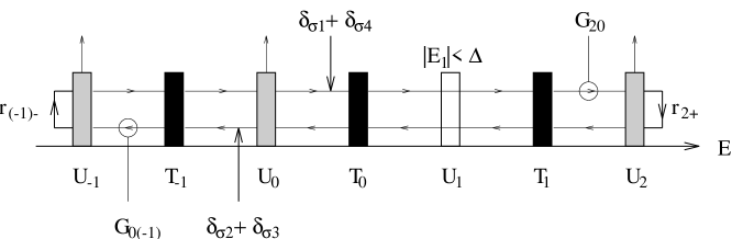
Fig.  3: Schematic structure of the mapping of the scattering state equations on a leaky one-dimensional Schrödinger potential. The ${\bf T}_{n}$-matrices introduce tunnel barriers (black boxes). Inside the energy gap, $|E_{n}|<\Delta$, the ${\bf U}_{n}$-matrices correspond to extra spacing (white box), while outside the gap they introduce leaking of particles out of the channel. The sources ($\delta_{\sigma 1}+\delta_{\sigma 4}$ and $\delta_{\sigma 1}+\delta_{\sigma 4}$) introduce particles into the potential structure and the amplitude for particles going away from the source are $G_{n0}$ and $G_{0(-n)}$, $n>0$. The particles are reflected from $\pm\infty$ with reflection amplitudes $r_{n\pm}$.

4 Formal solution

To solve Eqs. (12) one has to find two independent homogenous solutions that go to zero for $n=\pm\infty$ respectively, and then to match them at $n=0$. The boundary conditions,

$$\lim_{n\rightarrow\infty}{\bf M}_{nm}\hat{c}_{m+}=\mbox{\boldmath$0$}\hskip 8.5359pt(m\geq 0),\hskip 28.45274pt\lim_{m\rightarrow-\infty}({\bf M}_{nm})^{-1}\hat{c}_{n-}=\mbox{\boldmath$0$}\hskip 8.5359pt(n\leq 0),$$ (16)

fix the ratios $c^{\downarrow}_{n+}/c^{\uparrow}_{n+}=r_{n+}=\lim_{m\rightarrow\infty}r^{+}_{mn}$ for $n\geq 0$ and $c^{\uparrow}_{n-}/c^{\downarrow}_{n-}=r_{n-}=\lim_{m\rightarrow-\infty}r^{-}_{nm}$ for $n\leq 0$. The quantities $r_{n\pm}$ have the meaning of reflection amplitudes from $\pm\infty$ for upgoing and downgoing particles respectively.

We can now express the scattering state coefficients in terms of the matrices $S_{nm}$ and the reflection coefficients $r_{n\pm}$. We choose to give expressions for $\hat{c}_{n-}$ for $n>0$ and $\hat{c}_{n+}$ for $n<0$, knowing that Eq. (12) connects $\hat{c}_{n+}$ to $\hat{c}_{n-}$.

$$\hat{c}_{n-}=\frac{u_{0}^{2}-v_{0}^{2}}{u_{0}}\cdot\left[\delta_{1\sigma}+\delta_{2\sigma}a_{0}r^{l}_{0-}\right]\cdot G^{l}_{n0}\cdot\left(\begin{array}[]{c}1\\ a_{n}^{2}r^{l}_{n+}\end{array}\right)\hskip 8.5359pt(n>0),$$ (19)

$$\hat{c}_{n+}=\frac{u_{0}^{2}-v_{0}^{2}}{u_{0}}\cdot\left[\delta_{2\sigma}+\delta_{1\sigma}a_{0}r^{l}_{0+}\right]\cdot G^{l}_{0n}\cdot\left(\begin{array}[]{c}a_{n}^{2}r^{l}_{n-}\\ 1\end{array}\right)\hskip 8.5359pt(n<0).$$ (22)

The expressions for $\sigma\in\{3,4\}$ is found from Eq. (19) by the substitutions $l\rightarrow r$, $\delta_{1\sigma}\rightarrow\delta_{4\sigma}$ and $\delta_{2\sigma}\rightarrow\delta_{3\sigma}$. The expression for the quantity $G$ in the above equation reads

$$G_{nm}=\frac{t_{nm}}{(1-a_{m}^{2}r_{m-}r_{nm}^{+})(1-a_{n}^{2}r_{n+}r_{nm}^{-})-t_{nm}^{2}a_{m}^{2}a_{n}^{2}r_{m-}r_{n+}}\hskip 28.45274pt(n>m).$$ (23)

$G_{nm}$ is the dressed propagator, through source free regions of the multibarrier structure from point $m$ to point $n$ (see Fig. 3). The difference between the dressed propagator $G_{nm}$ and the bare transmission amplitude $t_{nm}$ is due to reflections from the region outside $[E_{m},E_{n}]$. Note that $G_{nm}$ in Eq. (23) is expressed through $r_{n+}$ and $r_{m-}$ (using the fact that the reflection amplitudes from the same sign of infinity are related by Eq. (14)). This form is vital for the cancellation theorem below (Eq. (30)).

5 dc Current

The total dc current through the junction has the form,

$$I_{dc}=\frac{e}{h}\int_{|E|>\Delta}dE\frac{|E|}{\sqrt{E^{2}-\Delta^{2}}}f(E)\sum_{\sigma}j^{\sigma}(E),$$ (24)

where the function $f(E)$ denotes the equilibrium population of the scattering states, originating from bulk electrodes. The current density $j^{\sigma}(E)$ has the form,

$$j^{\sigma}(E)=\sum_{n=-\infty}^{\infty}\left(|\alpha^{\sigma}_{n}(E)|^{2}-|\beta^{\sigma}_{n}(E)|^{2}+|\gamma^{\sigma}_{n}(E)|^{2}-|\delta^{\sigma}_{n}(E)|^{2}\right).$$ (25)

We can rewrite this in terms of the current flowing upwards in energy-space, $j_{n\pm}$,

$$j^{\sigma}(E)=\sum_{n=0}^{\infty}j^{\sigma}_{n+}(E)+\sum_{n=-\infty}^{0}j^{\sigma}_{n-}(E).$$ (26)

We note that for positive $n$ the current $j_{n\pm}$ is positive, while for negative $n$ it is negative, and therefore the two terms in the above equations have opposite signs. Using the boundary condition of vanishing coefficients for large $|n|$, we can rewrite the summation over $j_{n\pm}$ in Eq. (26) as a summation over probability currents $I^{p}_{n}(E)$,

$$j^{\sigma}(E)=\sum_{n\neq 0}nI^{p\sigma}_{n}(E).$$ (27)

We have now managed to separate the dc current into a weighted sum over probability currents transmitted from $E_{0}$ to $E_{n}$, where the weight $n$, is the number of times the probability current passes the junction. Since each Andreev reflection at energies within the superconducting gap is associated with the transfer of charge $2e$, Eq. (27) presents the total charge current as a sum over $n$-particle transmission processes [22].

The total probability current that flows between $E$ and $E_{n}$, including the superconducting density of states, is

$$I^{p}_{n}(E)=\frac{|E|}{\sqrt{E^{2}-\Delta^{2}}}\sum_{\sigma}I_{n}^{p\sigma}(E)=\displaystyle\sum_{\alpha\in\{l,r\}}(1-|a_{0}|^{2})(1-|a_{n}|^{2})|G^{\alpha}_{n0}|^{2}(1+|a_{n}r^{\alpha}_{n+}|^{2})(1+|a_{0}r^{\alpha}_{0-}|^{2}).$$ (28)

This current has no divergences, moreover by using the conservation law for probability current one finds that $I^{p}_{n}(E)\leq 4$. The form of the current in Eq. (28) can be interpreted in the following way. The current is proportional to the probability of transmission from $E$ to $E_{n}$, and the terms $(1-|a_{0}|^{2})$ and $(1-|a_{n}|^{2})$ are the probabilities to enter and leave the normal region respectively. Transmission from $E$ to $E_{n}$ consists of four alternative paths: direct transmission with the probability $|G_{n0}|^{2}$, transmission with excursion to and reflection from either minus infinity or plus infinity, which yields an additional factor $|a_{0}r_{0-}|^{2}$ or $|a_{n}r_{n+}|^{2}$ respectively, and finally transmission with excursions to and reflections from both minus infinity and plus infinity.

The probability current $I^{p}_{n}(E)$ in Eq. (28) obeys the important equation

$$I^{p}_{-n}(E)=I^{p}_{n}(E-neV),$$ (29)

which implies a detailed balance between probability currents flowing upwards and downwards in energy space respectively. This balance is straightforward to prove using the equality between $S_{nm}$ for quasiparticles incoming at $E+qeV$ and $S_{(n+q)(m+q)}$ for quasiparticles incoming at $E$. Using this detailed-balance equation one is able to prove the exact cancellation, at $T=0$, of currents which do not pass the energy gap,

$$\int_{-\infty}^{-\Delta-neV}I^{p}_{n}(E)dE-\int_{-\infty}^{-\Delta}I^{p}_{-n}(E)dE=0\hskip 28.45274pt(n>0).$$ (30)

This cancellation theorem proves the consistency of the single particle scattering approach to superconducting junctions. It is well known that within the Landauer-Büttiker scattering approach to elastic tunneling, e.g. in normal junctions [23, 24], the Pauli exclusion principle is automatically valid due to the exact cancellation of currents that do not produce real excitations. The cancellation theorem Eq. (30) extends this property to inelastic scattering (MAR) in superconducting junctions.

Using Eq. (30), and also the electron-hole symmetry of the BdG equation ($\sum_{\sigma}j^{\sigma}(-E)=-\sum_{\sigma}j^{\sigma}(E)$), we arrive at the final formula for the dc current at finite temperature,

$$I_{dc}=\sum_{n>0}n\left(\Theta(neV-2\Delta)\int_{\Delta-neV}^{-\Delta}dE[2f(E)-1]I^{p}_{n}(E)+2\int_{-\infty}^{-\Delta-neV}dE[f(E)-f(E_{n})]I^{p}_{n}(E)\right).$$ (31)

The obtained formula for the dc current in Eq. (31) has only positive terms and consists of two parts. The first part is related to the creation of real excitations, due to quasiparticles traversing the energy gap, and it is responsible for the SGS. This current exists at zero temperature and decreases with increasing temperature. The second part is a smooth background current from thermal excitations, and is exponentially small at low temperatures.

6 Subgap structure

Let us analyze SGS using Eqs. (23), (28) and (31). The magnitude of the $n$-particle current $I^{p}_{n}(E)$ is proportional to the transmittivity $|t_{n0}|^{2}$ of the $n$-barrier tunnel structure, which is estimated as $|t_{n0}|^{2}\propto D^{n}$ in the absence of resonances, where $D$ is the transmissivity of the normal junction. Therefore, the current in Eq. (31) consists of a step-like structure with the onsets at $eV=2\Delta/n$. This step-like structure is particularly pronounced in junctions with low transmittivity $D\ll 1$ [7], and it is washed out in transparent junctions with $D\approx 1$. However, even in the latter case, the current decreases exponentially at low voltages, $I_{dc}\propto D^{2\Delta/eV}$, as soon as $D\neq 1$ [9].

This simple step-like structure is complicated by resonances in $I^{p}_{n}(E)$. One may distinguish three different sources of resonant behaviour. First there may be normal electron resonances in the transfer matrices $T_{n}$ [12, 14, 15].

Secondly, even in the absence of normal electron resonances there are specific superconducting resonances in the bare transmission amplitudes $t_{n0}$ due to electron-hole dephasing during transmission through long junctions and during Andreev reflections given by matrices $U$. In the mapping, dephasing is a source of phase gained between the barriers in Fig. 3. In short constrictions, $L=0$, the resonant condition reads $arg(a_{k})=m\pi$, where $m$ is integer, and it is fulfilled near the gap edges, $E_{k}\approx\pm\Delta$. (For energies outside the gap the phase gained is constant, $\pm\pi$, but for $|E/\Delta|-1>D^{2}$ the resonance vanishes because of the leakage.) The resonance effectively removes two barriers so the bare transmission probability is increased by the factor $D^{-2}$. It is easy to see that at voltages $eV=2\Delta/n$ it is possible to have simultaneously two resonances with corresponding indices related as $k^{\prime}=k+n$. In this case the transmission probability $|t_{n0}|^{2}$ is enhanced by the factor $D^{-3}$ if the resonances are next to each other ($n=1$), otherwise the enhancement factor is $D^{-4}$.

Finally there are the resonances due to reflection from $\pm\infty$ in the denominator of Eq. (23), boundary resonances. The conditions for resonance are $(1-a_{0}^{2}r_{0-}r_{n0}^{+})=0$ and $(1-a_{n}^{2}r_{n+}r_{n0}^{-})=0$, which is possible for $E=-\Delta$ or $E_{n}=\Delta$ respectively. These resonances are only important when they overlap with resonances in the bare transmission amplitude. An interplay of the resonances in the bare transmission amplitude $t_{n0}$ and the boundary resonances produces current peaks in the subharmonic gap structure (Fig. 4).

As an example of this interplay let us discuss the 4-particle current in a short junction , which possesses all typical features. The 4-particle current ($I_{4}$) (see Fig. 4) has an onset at $2\Delta/eV=4$. In the voltage region $3<2\Delta/eV<4$ there are no resonances in $t_{40}$ and therefore the magnitude of the current is $I_{4}\propto D^{4}$. For voltages $2\Delta/eV<3$ a single resonance in $t_{40}$ becomes possible, which gives an enhancement of the current to $I_{4}\propto D^{4}|ln(D)|$. Close to $2\Delta/eV=3$ this resonance overlaps with a boundary resonance which results in a current peak with the magnitude $(I_{4})_{max}\propto D^{3}$. At $2\Delta/eV=2$ there is a double resonance, $E_{1}=-\Delta$ and $E_{3}=\Delta$, which results in a current peak of order $(I_{4})_{max}\propto D^{2}$. The voltage $2\Delta/eV=1$ is a special case because the two resonances are next to each other so the enhancement of the transmission probability is only $D^{-3}$, resulting in a current peak $(I_{4})_{max}\propto D^{3}$. At this voltage the 4-particle current is weakened by the leaky Andreev reflection outside the gap.

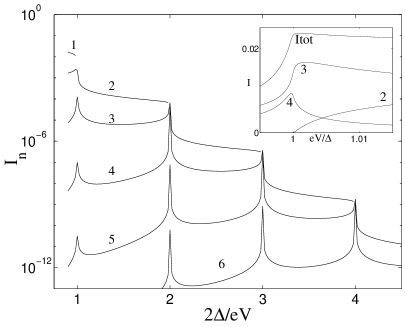
Fig.  4: The SGS of a SIS junction with transparency $D=0.01$ divided into different $n$-particle currents, for $n\in\{1,6\}$. The inset shows the SGS of a SIS junction with transparency $D=0.1$ close to $eV=\Delta$ and the contributions from 2-, 3- and 4-particle currents.

7 Conclusions

In conclusion, we have presented an approach, for analyzing the SGS in quantum superconducting junctions, where MAR is treated as a transport problem in energy space. Such an approach is natural for the inelastic scattering problem represented by MAR. Using scattering theory formalism, we have derived a mapping of MAR onto a problem of transmission through a 1D wave guide with a built in multiple tunnel barrier structure. There is no current conservation in this transmission problem due to a leakage outside the wave guide. The charge current in the original superconducting junction is expressed through this leakage, which is identical to the probability current of outgoing quasiparticles in the superconductors. In terms of such a mapping, the SGS is explained in terms of resonances in the transmission along the energy axis. Three different types of resonances have been found which are important for the interpretation of SGS: (i) superconducting resonances induced by electron-hole dephasing and the Andreev reflections, (ii) boundary resonances induced by reflections from the boundaries of the wave guide, and (iii) normal electron (Breit-Wigner) resonances, which may exist in addition to former two types of the resonances, which are always present in MAR. The mapping allowed us to separate currents associated with $n$-particle transmission processes and to prove the cancellation of non-physical ground state currents, which is equivalent to the Pauli exclusion principle.

References

- [1] T.M. Klapwijk, G.E. Blonder and M. Tinkham, Physica B+C, 109-110, 1657 (1982).
- [2] G.B. Arnold, J. Low Temp. Phys. 68, 1 (1987).
- [3] U. Gunsenheimer and A.D. Zaikin, Phys. Rev. B 50, 6317 (1994).
- [4] B.A. Aminov, A.A. Golubov, and M.Yu. Kupriyanov, Phys. Rev. B 58, 365 (1996).
- [5] J.C. Cuevas, A. Martin-Rodero, and A. Levy Yeyati, Phys. Rev. B 54, 7366 (1996).
- [6] R. Kümmel, U. Gunsenheimer and R. Nicolsky, Phys. Rev. B 42, 3992 (1990).
- [7] E.N. Bratus’, V.S. Shumeiko, and G.Wendin, Phys. Rev. Lett. 74, 2110 (1995).
- [8] V.S. Shumeiko, E.N. Bratus’, and G. Wendin, Low Temp. Phys. 23, 249 (1997).
- [9] E.N. Bratus’, V.S. Shumeiko, E.V. Bezuglyi, and G. Wendin, Phys.Rev. B 55, 12666 (1997).
- [10] D. Averin and A. Bardas, Phys. Rev. Lett. 75, 1831 (1995).
- [11] M. Hurd, S. Datta and P. F. Bagwell, Physical Review B 54, 6557 (1996)
- [12] A. Levy Yeyati, J.C. Cuevas, A. Lopez-Davalos, and A. Martin-Rodero, Phys. Rev. B 55, R6317 (1997).
- [13] A. Golub, Phys. Rev. B 52, 7458 (1995).
- [14] G. Johansson, E. Bratus’, V.S. Shumeiko, and G. Wendin, Physica C 293, 77 (1997).
- [15] G. Johansson, V.S. Shumeiko, E.N. Bratus, and G. Wendin, cond-mat 9807240.
- [16] M. Hurd, Phys. Rev. B 55, R11993 (1997); M. Hurd, T. Löfwander, G. Johansson and G. Wendin, cond-mat 9807081 (1998).
- [17] A.W. Kleinsasser, R.E. Miller, W.H. Mallison and G.B. Arnold, Phys. Rev. Lett. 72, 1738 (1994).
- [18] N. van der Post, E.T. Peters, I.K. Yanson and J.M. van Ruitenbeek, Phys. Rev. Lett. 73, 2611 (1994).
- [19] N. van der Post, PhD Thesis, Leiden, 1997.
- [20] E. Scheer, P. Joyez, M.H. Devoret, D. Esteve, and C. Urbina, Phys. Rev. Lett. 78, 3535 (1997).
- [21] E. Scheer et al, Nature 394, 154 (1998).
- [22] J.R. Schrieffer and J.W. Wilkins, Phys. Rev. Lett. 10, 17 (1963).
- [23] R. Landauer, IBM J. Res. Dev. 1, 223 (1957).
- [24] M.A. Büttiker, Phys. Rev. Lett. 57, 1761 (1986).
- [25] T. Löfwander, G. Johansson, V. Shumeiko, and G. Wendin, in this issue.