Spin polarons in triangular antiferromagnets

Abstract

The motion of a single hole in a 2D triangular antiferromagnet is investigated using the $t$-$J$ model. The one-hole states are described by strings of spin deviations around the hole. Using projection technique the one-hole spectral function is calculated. For large $J/t$ we find low-lying quasiparticle-like bands which are well separated from an incoherent background by a gap of order $J$. However, for small $J/t$ this gap vanishes and the spectrum becomes broad over an energy range of several $t$. The results are compared with SCBA calculations and numerical data.

Since the discovery of high-temperature superconductivity, charge carriers in doped antiferromagnets (AF) have been studied intensively. A reliable description of the hole motion is important for the understanding of the low-energy charge dynamics in the copper-oxide planes of the cuprate superconductors. A large number of numerical and analytical studies indicate that a single hole in an AF spin background has nontrivial properties: The spectral function consists of a pronounced coherent peak at the bottom of the spectrum and a incoherent background at larger energies. The coherent peak can be associated with the motion of a dressed hole, i.e., a hole surrounded by spin defects (”spin polaron”)  [1, 2, 3, 4, 5, 6].

Materials with spin arrangements on 2D non-square lattices have also been synthetized. For example, experiments suggest the realization of a triangular spin-$1\over 2$ AF in NaTiO₂ [7], as well as in surface structures [8] such as K/Si(111):B. Delafossite cuprates RCuO_2+δ, with R a rare-earth element, have Cu ions sitting on a triangular lattice [9]. Furthermore, recent results in the context of organic superconductors indicate that $\kappa$-(BEDT-TTF)₂X, where X is an ion, may be described by a half-filled Hubbard model on an anisotropic triangular lattice [10].

Although most of these materials do not contain a finite concentration of holes or electrons away from half-filling, it is of fundamental theoretical interest to study the hole dynamics in this environment. In this paper we adress the motion of a single hole in an otherwise half-filled system. The one-hole spectral function for this case corresponds directly to the result of an angle-resolved photoemission experiment (ARPES) on the undoped compound.

We assume that a triangular AF doped with holes is well described by the $t$-$J$ model on a triangular lattice,

$$H\,=\,-t\sum_{\langle ij\rangle\sigma}({\hat{c}}^{\dagger}_{i\sigma}{\hat{c}}_{j\sigma}+{\hat{c}}^{\dagger}_{j\sigma}{\hat{c}}_{i\sigma})+J\sum_{\langle ij\rangle}\ {\bf S}_{i}\cdot{\bf S}_{j}$$ (1)

in standard notation. Note that, in contrast to the square lattice, there is no electron-hole symmetry for the triangular lattice $t$-$J$ model, i.e., the physics depends on the sign of $t$. For half-filling this model reduces to the triangular Heisenberg antiferromagnet (THAF) with spins $1\over 2$[11]. It is by now widely believed that its ground state possesses magnetic long-range order [12, 13] which can be described as the 120^o order being the ground state of the classical spin model (Fig. 1) with additional quantum fluctuations.

FIG. 1.: a) The classical ground state of the triangular AF together with the three unit vectors ${\bf e}_{i}$ of the lattice. The 120^o spin order defines three sublattices A, B, and C. b) Brillouin zone for the triangular system with the path in momentum space for the following figures.

To investigate the hole motion we consider a one-particle Green’s function describing the creation of a single hole with momentum $\bf k$ at zero temperature:

$$G({\bf k},\omega)\;=\;\sum_{\sigma}\langle\psi_{0}^{N}|{\hat{c}}_{{\bf k}\sigma}^{\dagger}{1\over{z-L}}{\hat{c}}_{{\bf k}\sigma}|\psi_{0}^{N}\rangle$$ (2)

where $z$ is the complex frequency variable, $z=\omega+i\eta$, $\eta\rightarrow 0$. The quantity $L$ denotes the Liouville operator defined by $LA=[H,A]_{-}$ for arbitrary operators $A$. $|\psi_{0}^{N}\rangle$ is the ground state of undoped system, i.e., with $N$ electrons on $N$ lattice sites.

The one-hole problem in the triangular lattice has up to now analytically only been studied [14, 15] using self-consistent Born approximation (SCBA). The SCBA (without vertex corrections) neglects spiral loops in the hole motion (Trugman processes[3]) since they are formally crossing diagrams. However, for the triangular lattice these processes are expected to be more important than for the square lattice since only three hopping steps are necessary for one loop. Here we prefer another analytical approach which is based on the picture of the spin-bag quasiparticle (QP) or magnetic polaron [2, 3, 4, 5, 6]. The spin deviations surrounding the hole are described by a set of path operators [2, 3, 4, 5]. The correlation function (2) can be evaluated using a cumulant version [16, 17] of Mori-Zwanzig projection technique[18].

In the calculations of this paper the ground state $|\psi_{0}^{N}\rangle$ of the undoped THAF is assumed to be long-range ordered [12, 13]. Its description is based on an expansion around the classical ground state $|\phi_{\rm cl}\rangle$ of the triangular antiferromagnet, see Fig. 1. Translational invariance and rotation invariance in spin space are spontaneously broken; we choose the coordinates that the spins in $|\phi_{\rm cl}\rangle$ are arranged in the $x$-$z$ plane.

For the analytical treatment we locally rotate all spins to transform the classical ground state into a formally ferromagnetic state. The rotation is carried out around the $y$-axis by an angle of ${\bf Q}\cdot{\bf R}_{i}$ with ${\bf Q}=({8\over 3}\pi,0)$ at site $i$. The ”original” electron operators ${\hat{c}}^{(\dagger)}$ and the ”new” operators ${\hat{d}}^{(\dagger)}$ in the rotated basis are related through:

$${\hat{c}}_{i\sigma}\;=\;\cos\frac{{\bf Q}\cdot{\bf R}_{i}}{2}\>{\hat{d}}_{i\sigma}+\sin\frac{{\bf Q}\cdot{\bf R}_{i}}{2}\>{\hat{d}}_{i,-\sigma}\,.$$ (3)

The resulting Hamiltonian $H=H_{0}+H_{1}$ has the following form:

$$H_{0} \;=\; +{t\over 2}\sum_{\langle ij\rangle\sigma}({\hat{d}}^{\dagger}_{i\sigma}{\hat{d}}_{j\sigma}+{\hat{d}}^{\dagger}_{j\sigma}{\hat{d}}_{i\sigma})\,+\,{J\over 2}\sum_{\langle ij\rangle}\ T_{i}^{z}T_{j}^{z}$$ (4)

$$H_{1} \;=\; -\,{t\sqrt{3}\over 2}\sum_{\langle i\rightarrow j\rangle\sigma}\sigma({\hat{d}}^{\dagger}_{i\sigma}{\hat{d}}_{j,-\sigma}-{\hat{d}}^{\dagger}_{j\sigma}{\hat{d}}_{i,-\sigma})$$ (7)

$$+\,{J\over 8}\sum_{\langle ij\rangle}\ \left(T_{i}^{-}T_{j}^{+}\,-\,3T_{i}^{+}T_{j}^{+}+{\rm h.c.}\right)$$

$$+\,{J\sqrt{3}\over 4}\sum_{\langle i\rightarrow j\rangle}\ \left[T_{i}^{z}(T_{j}^{+}+T_{j}^{-})\,-\,T_{j}^{z}(T_{i}^{+}+T_{i}^{-})\right]\,.$$

${\hat{d}}^{(\dagger)}$ are the electron destruction (creation) operators in the rotated basis, $T$ are the corresponding spin operators. Like in the original $t$-$J$ model the operators ${\hat{d}}^{(\dagger)}$ exclude double occupancies. The summation symbol $\langle i\rightarrow j\rangle$ refers to orientated pairs $\langle ij\rangle$ where the link $i\rightarrow j$ runs in positive direction with respect to one of the unit vectors ${\bf e}_{i}$ of the lattice. The ground state of $H_{0}$ is now ferromagnetic, whereas $H_{1}$ contains the fluctuations. An important difference compared to the square-lattice hole motion problem is the existence of a direct hopping term (in $H_{0}$), i.e., hopping without creation of a background spin-defect. This follows from the fact that the spin states on adjacent sites in the classical ground state are not exactly orthogonal.

The hole motion processes will be described in the concept of path operators  [2, 3, 5] which create strings of spin fluctuations attached to the hole. For the application of projection technique we define a set of path operators $\{A_{I}\}$ which couple to a hole and create local spin defects with respect to the classical ground state. The first operator $A_{0}$ is the unity operator, the second one $A_{1}$ moves the hole by one lattice spacing creating one spin defect and so on. We are interested in calculating dynamical correlation functions for the operators $\{A_{I}{\hat{c}}_{{\bf k}\sigma}\}$:

$$G_{I\sigma,J\sigma^{\prime}}(z)\,=\,\langle\psi_{0}^{N}|\,(A_{I}{\hat{c}}_{{\bf k}\sigma})^{\dagger}{1\over{z-L}}(A_{J}{\hat{c}}_{{\bf k}\sigma^{\prime}})^{\phantom{\dagger}}\,|\psi_{0}^{N}\rangle\,.$$ (8)

The Green’s function (2) for the physical hole is then given by $\sum_{\sigma}G_{0\sigma,0\sigma}(z)$. Note that it is equivalent to consider correlation functions for operators $\{A_{I}{\hat{d}}_{{\bf k}\sigma}\}$; then the physical Green’s function (2) has to be calculated using relation (3). Using cumulants the correlation functions $G$ can be rewritten as [17]:

$$G_{I\sigma,J\sigma^{\prime}}(z)\,=\,\langle\phi_{\rm cl}|\,\Omega^{\dagger}\,(A_{I}{\hat{c}}_{{\bf k}\sigma})^{\dagger}\left({1\over{z-L}}A_{J}{\hat{c}}_{{\bf k}\sigma^{\prime}}^{\phantom{\dagger}}\right)^{\cdot}\,\Omega\,|\phi_{\rm cl}\rangle^{c}\,.$$ (9)

The brackets $\langle\phi_{\rm cl}|\,...\,|\phi_{\rm cl}\rangle^{c}$ denote cumulant expectation values with $|\phi_{\rm cl}\rangle$. The dot $\cdot$ in Eq. (9) indicates that the quantity inside $(...)^{\cdot}$ has to be treated as a single entity in the cumulant formation. The operator $\Omega$ transforms $|\phi_{\rm cl}\rangle$ being the ground state of $H_{0}$ into the exact ground state $|\psi_{0}^{N}\rangle$ of $H=H_{0}+H_{1}$ at half-filling. Here $\Omega$ is approximated with an exponential ansatz which introduces spin fluctuations into $|\phi_{\rm cl}\rangle$:

$$|\psi_{0}^{N}\rangle\>=\>\Omega\,|\phi_{\rm cl}\rangle\>=\>\exp\left(\sum_{\nu}\alpha_{\nu}S_{\nu}\right)|\phi_{\rm cl}\rangle\,.$$ (10)

The operators $S_{\nu}$ describe the effect of the spin-flip terms in $H_{1}$. This approach has been shown to give reasonable results for the square lattice AF [16]. Here operators with up to 4 spin defects with a maximum distance of 4 lattice spacings have been employed. Following ref. [19] one obtains a non-linear set of equations for the coefficients $\alpha_{\nu}$, $0=\langle\phi_{\rm cl}|S_{\nu}^{\dagger}\,H\,\Omega\,|\phi_{\rm cl}\rangle^{c}$, which can be solved self-consistently.

Using Mori-Zwanzig projection technique [18] one can derive a set of equations of motion for the dynamical correlation functions $G_{I\sigma,J\sigma^{\prime}}(z)$. Neglecting the self-energy terms it reads:

$$\sum_{I\sigma}\Omega_{K\tilde{\sigma},I\sigma}(z)\,G_{I\sigma,J\sigma^{\prime}}(z)\,\,=\,\,\chi_{K\tilde{\sigma},J\sigma^{\prime}}\,,$$ (11)

$$\Omega_{K\tilde{\sigma},J\sigma^{\prime}}(z)=z\delta_{KJ}\delta_{\tilde{\sigma}\sigma^{\prime}}-\sum_{L\sigma^{\prime\prime}}\omega_{K\tilde{\sigma},L\sigma^{\prime\prime}}^{\phantom{-1}}\,\chi_{L\sigma^{\prime\prime},J\sigma^{\prime}}^{-1}\,.$$ (12)

$\chi_{I\sigma,J\sigma^{\prime}}$ and $\omega_{I\sigma,J\sigma^{\prime}}$ are the static correlation functions and frequency terms, respectively. They are given by the following cumulant expressions:

$$\chi_{I\sigma,J\sigma^{\prime}} = \langle\phi_{\rm cl}|\Omega^{\dagger}(A_{I}{\hat{c}}_{{\bf k}\sigma})^{\cdot\dagger}(A_{J}{\hat{c}}_{{\bf k}\sigma^{\prime}})^{\cdot}\Omega\,|\phi_{\rm cl}\rangle^{c}\,,$$ (13)

$$\omega_{I\sigma,J\sigma^{\prime}} = \langle\phi_{\rm cl}|\Omega^{\dagger}(A_{I}{\hat{c}}_{{\bf k}\sigma})^{\cdot\dagger}\left(L(A_{J}{\hat{c}}_{{\bf k}\sigma^{\prime}})^{\phantom{\dagger}}\right)^{\cdot}\Omega\,|\phi_{\rm cl}\rangle^{c}\,.$$ (14)

These terms describe all dynamic processes within the subspace of the Liouville space spanned by the operators $\{A_{I}{\hat{c}}_{{\bf k}\sigma}\}$. The use of cumulants ensures size-consistency, i.e., only spin fluctuations connected with the hole enter the final expressions for the one-hole correlation function. In the present calculations we have employed up to 900 projection variables with a maximum paths length of 4. The neglection of the self-energy terms leads to a discrete set of poles for the Green’s functions, in all figures we have introduced an artificial linewidth to plot the spectra. For details of the calculational procedure see e.g. [5].

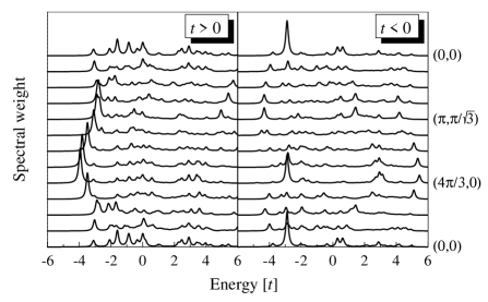
FIG. 2.: One-hole spectral function for $J/|t|=0.5$ and different momenta; left: positive $t$, right: negative $t$. The energies are measured relative to the energy of a localized hole; the path in the Brillouin zone is shown in Fig. 1.

Now we turn to the discussion of the results. The one-hole spectral function ${\rm Im}\,G({\bf k},\omega)$ for both positive and negative $t$ and different momenta is shown in Figs. 2 - 4 ($J/t=$ 0.5, 2.0, and 10.0). For large $J/t$ we observe pronounced low-lying QP bands and additional excitations with low weight at higher energies which form an incoherent background. With decreasing $J/t$ the gap between the QP band and the background excitations decreases. For $J/t=0.5$ this gap is almost vanished, furthermore a sharp QP peak is only present near the bottom of the QP band. Values of $J/t\leq 0.2$ lead to a incoherent spectrum.

For negative $t$ the character of the spectral function is in principle similar to the $t>0$ results, i.e., for large $J/|t|$ ($\geq 1.0$) the QP peak is well defined, whereas for small $J/|t|$ the spectra become incoherent.

FIG. 3.: Same as Fig. 2 but for $J/|t|=2.0$.

Next we are going to examine the properties of the low-lying bands. Fig. 5 shows the dispersion $\epsilon_{\bf k}$ of the lowest pole for positive $t$ and different $J/t$ in comparison with data from the literature. For $t>0$ the band has its energy minimum at momentum $({4\over 3}\pi,0)$ and equivalent points. For $t<0$ and large $J/|t|\geq 4$ the situation is similar to the positive $t$ case with the dispersion of the QP band reversed, see Fig. 4. However, for intermediate $J/|t|$ and $t<0$ the QP dispersion almost vanishes (Fig. 3). This can be explained from the composite nature of the hole motion process in the triangular system. The motion consists of direct hopping [amplitude $t/2$, cf. eq. (7)] and spin-fluctuation-assisted hopping (like in the square lattice) with an amplitude being nearly independent of the sign of $t$ (since the main contribution contains two hopping steps and one spin-flip process). For negative $t$ these two contributions to the dispersion tend to cancel each other leading to the very narrow band at $J/|t|=2.0$.

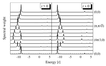
FIG. 4.: Same as Fig. 2 but for $J/|t|=10.0$.

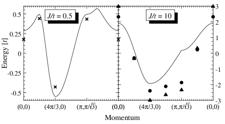
FIG. 5.: Dispersion of the low-lying QP band for $t>0$. Left: $J/|t|=0.5$, present calculation (solid) and ED data (12 sites, crosses) taken from ref. [14]. Right: $J/|t|=10$, present calculation (solid) together SCBA data (dots) and ED data (21 sites, triangles) from ref. [15]. The energy zero level has been set at the center of mass of the band.

Another interesting feature is the splitting of the QP band into two which is especially visible at large $J/|t|$. It is related to the non-collinear magnetic long-range order in the system and can be understood as follows: The states $|\phi_{\rm cl}\rangle$ and $|\phi_{0}^{N}\rangle$ have a non-zero helicity, therefore both $y$ directions in spin space (perpendicular to the plane defined by the spin directions in $|\phi_{\rm cl}\rangle$) are not equivalent. The analysis of the eigenvectors of the dynamic matrix $\Omega_{I\sigma,J\sigma^{\prime}}$ shows that the one-hole eigenmodes correspond to states where the missing spin has a definite $y$ component. (These are no eigenstates of $S_{z}^{\rm tot}$.) These two modes have different energies (for a given ${\bf k}$) which leads to two distinct bands in the spin-integrated spectral function (2). A spin-resolved photoemission experiment (with spins parallel or antiparallel to the helicity direction) should observe one or the other of these bands.

The one-hole dispersion for $J/t=0.5$ calculated here is in quantitative agreement with exact diagonalization (ED) data on a 12-site cluster [14]. The $J/t=10$ dispersion curve agrees with recent results which where obtained using the SCBA technique and ED on a 21-site cluster [15] (see Fig. 5). To compare results, one has to take into account an overall shift of the hole momenta by $({4\over 3}\pi,0)$ between clusters with odd and even number of sites.

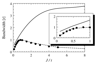
FIG. 6.: Comparison of the hole QP bandwidth in triangular and square lattice antiferromagnets. Solid/dashed: Triangular/square lattice, present calculation. Circles: Square lattice SCBA results from ref. [6]. Inset: $J$ range from 0 to 1.

Finally we want to compare the QP bandwidth with the one found for the square lattice hole motion. In Fig. 6 we have plotted the bandwidth for both systems depending on the ratio $J/t$. For the square lattice it is known [4, 5, 6] that the bandwidth for small $J/t$ ($<1$) is essentially given by $J$ since hole hopping always creates spin defects with respect to the AF background. These defects have to be ”repaired” by the transverse part of the Heisenberg exchange with energy scale $J$. In contrast, in the triangular lattice the bandwidth for small $J/t$ is given by $at+bJ$, whereas for large $J/t$ values it saturates at $4.5\,t$. This behavior follows from the existence of the direct hopping term with prefactor $t/2$ in $H_{0}$ (7) which has been discussed above. It leads to a disperison proportional to $t$; the saturation bandwidth is half of the bandwidth of the uncorrelated system ($9\,t$). Additional hole motion processes accompanied by spin fluctuations lead to a dispersion proportional to $J$ (at small $J/t$) as in the square lattice. So the physical picture for the hole quasiparticle is the following: At small and intermediate $J/t$ the hole is surrounded by spin fluctuations, the dynamics consists of coherent quasiparticle motion and of incoherent processes within the quasiparticle (which dominate the spectrum at small $J/t$). At large $J/t$ spin fluctuations are suppressed, but the direct hopping term allows the hole to move without creating background spin defects. So the pure hole hops with $t/2$ as a (nearly) free fermion.

Summarizing, we have studied the one-hole motion in a triangular AF described by the $t$-$J$ model. Using the spin-polaron concept which describes the hole states in terms of local spin defects we find that the one-hole spectral function shows a QP peak for sufficiently large $J/|t|$. In this regime the picture of a mobile hole dressed by spin fluctuations (known from the square lattice) also applies to the triangular system. The QP dispersion arises both from direct and spin-flip-assisted hopping processes which leads to differences between the $t>0$ and $t<0$ cases. For small $J/|t|$ the one-hole spectra become incoherent, i.e., the QP weight decreases and the gap between the QP band and the background formed by additional magnetic excitations vanishes.

Note that the addition of more than one hole to a triangular AF may lead to hole pairing induced by spin-wave exchange [20] which is likely relevant for organic superconductors [10].

The author thanks K. W. Becker and E. Dagotto for useful conversations. Support by the DAAD (D/96/34050) and the hospitality of the NHMFL (Tallahassee) are gratefully acknowledged.

REFERENCES

- [1] E. Dagotto, Rev. Mod. Phys. 66, 763 (1994).
- [2] Y. Nagaoka, Phys. Rev. 147, 392 (1966), W. F. Brinkman and T. M. Rice, Phys. Rev. B 2, 1324 (1970), B. I. Shraiman and E. D. Siggia, Phys. Rev. Lett. 60, 740 (1988).
- [3] S. A. Trugman, Phys. Rev. B 37, 1597 (1988).
- [4] J. A. Riera and E. Dagotto, Phys. Rev. B 55, 14543 (1997).
- [5] M. Vojta and K. W. Becker, Phys. Rev. B 57, 3099 (1998).
- [6] G. Martinez and P. Horsch, Phys. Rev. B 44, 317 (1991).
- [7] K. Hirakawa , J. Phys. Soc. Jpn. 54, 3526 (1985); K. Takeda , 61, 2156 (1992).
- [8] H. H. Weitering , Phys. Rev. Lett. 78, 1331 (1997).
- [9] R. Cava , J. Solid State Chem. 104, 437 (1993); A. Ramirez , Phys. Rev. B 49, 16082 (1994).
- [10] R. H. McKenzie, Science 278, 820 (1997).
- [11] P. Fazekas and P. W. Anderson, Phil. Mag. 30, 423 (1974).
- [12] R. R. P. Singh and D. Huse, Phys. Rev. Lett. 68, 1766 (1992).
- [13] B. Bernu et , Phys. Rev. B 50, 10048 (1994).
- [14] M. Azzouz and T. Dombre, Phys. Rev. B 53, 402 (1996).
- [15] W. Apel, H.-U. Everts, and U. Körner, Eur. Phys. J. B 5, 317 (1998).
- [16] K. W. Becker and P. Fulde, Z. Phys. B 72, 423 (1988).
- [17] K. W. Becker and W. Brenig, Z. Phys. B 79, 195 (1990).
- [18] H. Mori, Progr. Theor. Phys. 34, 423 (1965), R. Zwanzig, in: Lectures in Theoretical Physics vol. 3. New York: Interscience 1961.
- [19] T. Schork and P. Fulde, J. Chem. Phys. 97, 9195 (1992).
- [20] M. Vojta and E. Dagotto, preprint cond-mat/9807168, J. Schmalian, Phys. Rev. Lett. 81, 4232 (1998).