A Mesoscopic Quantum Eraser

Abstract

Motivated by a recent experiment by Buks et al. [Nature 391, 871 (1998)] we consider electron transport through an Aharonov–Bohm interferometer with a quantum dot in one of its arms. The quantum dot is coupled to a quantum system with a finite number of states acting as a which–path detector. The Aharonov–Bohm interference is calculated using a two–particle scattering approach for the joint transitions in detector and quantum dot. Tracing over the detector yields dephasing and a reduction of the interference amplitude. We show that the interference can be restored by a suitable measurement on the detector and propose a mesoscopic quantum eraser based on this principle.

Recent progress in quantum and atom optics has made it possible to test basic tenets of quantum physics. Complementarity has been tested in various realizations [1] of the classical double–slit gedanken experiment using photon pairs created in parametric down–conversion. Related experiments [2] utilizing atomic beams instead of photons have been performed very recently. These experiments not only confirmed the destruction of multiple–path interference due to a which–path measurement. More importantly, they also demonstrated that the loss of interference need not be irreversible if the which-path detector is itself a quantum system. In fact, realizing Scully’s [3] idea of a quantum eraser it was shown that the interference can be restored by erasing the which-path information from the detector in a subsequent measurement. Quantum detectors which have been used in practical implementation of quantum erasers include the photon polarization and internal degrees of freedom of atoms in an atomic beam.

In this Letter, we address the measurement process and the concept of a quantum eraser in the domain of mesoscopic physics. Specifically, we propose a semiconductor microstructure which can act as a quantum eraser. Far from only duplicating and/or corroborating results in optics, such a device would be of considerable interest in its own right. First, it would test quantum physics in the domain of solid state physics. Second, and in contrast to quantum optics, mesoscopic probes are inevitably coupled to macroscopic bodies (leads etc.), opening the possibility to address quantitatively the issue of quantum decoherence. Finally, mesoscopic probes offer the possibility of practical applications.

Our work is motivated by the first demonstration of controlled dephasing in a which–path semiconductor device by Buks et al. [4]. In a pioneering experiment, the authors used an Aharonov-Bohm (AB) interferometer with a quantum dot (QD) embedded in one of the arms. The coherent transmission of electrons through the QD was detected by the capacitive change of the transmission of a quantum point contact (QPC) located in the immediate vicinity of the dot. Theoretical work on this experiment employs a rate equation formalism [5], a change of the quantum state of the environment of the dot [4], dephasing of the electron on the dot by the environment [6], and creation of both virtual and real excitations in the QPC [7].

In the experiment by Buks et al., the QPC serves as a dephasing device and tests complementarity. Theoretically, this situation is described by accounting for the coupling between QD and QPC, and by tracing over the states of the QPC. However, while this procedure generates dephasing in the AB–ring it does not provide any information about the actual path of the electrons through the AB–ring. To obtain such information an additional measurement must be performed on the quantum detector coupled to the AB–ring. It is the purpose of the present paper to investigate the influence of such a true which–path measurement on the interference contrast. We address this question by coupling an AB–ring to a quantum detector with a finite number of states (see Fig. 1)). Such a discrete quantum detector can be realized e.g. by utilizing the spin of the electron passing through the QD, or by a pair of quantum dots coupled capacitively to the QD in the AB interferometer. An electron passing through the AB interferometer leaves which–path information in the detector by changing its quantum state. We derive the AB–contrast using a novel two–particle scattering approach for joint transitions through the AB–ring and in the detector. Analyzing various possible measurements we show that the detector with the AB–ring can be used as a quantum eraser, i.e., a setup which allows to erase part or all of the which–path information stored in the detector.

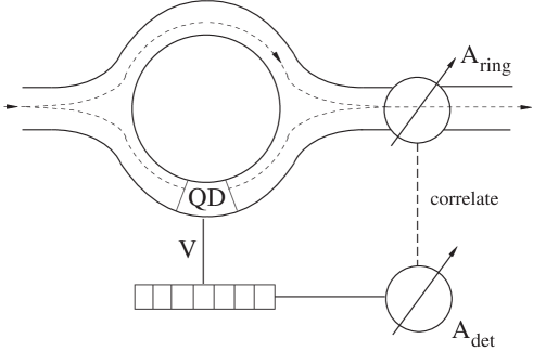
Fig. 1.–: Schematic view of the mesoscopic quantum eraser. An Aharonov–Bohm interferometer with a quantum dot is coupled to a discrete quantum detector via the interaction $V$. The measurement of the electron transmission $A_{\rm ring}$ through the interferometer is correlated with the measurement $A_{\rm det}$ performed on the detector.

We assume that the QD is in the Coulomb blockade regime and sufficiently close to a resonance so that only a single dot state need be considered. Energy and width of this resonance in the absence of any coupling to the quantum detector are denoted by $E_{0}$ and $\Gamma$, respectively. Let $\alpha,\alpha^{\prime}$ denote the leads coupled to the AB interferometer and $p,p^{\prime}$ the transverse modes in the leads. Then, $c\equiv\{p\alpha\}$ denotes the channels with $\delta_{cc^{\prime}}=\delta_{pp^{\prime}}\delta_{\alpha\alpha^{\prime}}$. We recall that without coupling to the quantum detector, the scattering matrix $S^{\rm AB}_{cc^{\prime}}$ for passage of an electron through the AB–interferometer is given by [8]

$$S^{\rm AB}_{cc^{\prime}}=\left(S^{(0)}_{cc^{\prime}}-2\pi i{\gamma_{c}\gamma_{c^{\prime}}\over E\!-\!E_{0}\!+\!i\Gamma/2}\right)\ .$$ (1)

We have introduced the total energy $E$, and the partial width amplitudes $\gamma_{c}$, $\gamma_{c^{\prime}}$ for decay of the QD resonance into the channels $c$, $c^{\prime}$, respectively. The term $S^{(0)}$ describes an energy– and flux–independent background due to scattering through that arm of the AB–interferometer which does not contain the QD. The last term in Eq. (1) accounts for all scattering processes through the QD including multiple scattering through the AB–ring. This term depends on the magnetic flux $\Phi$ threading the AB–ring through the partial width amplitudes $\gamma_{c}$, $\gamma_{c^{\prime}}$ and the total width $\Gamma$ [9]. The flux–dependence is non–trivial in general since it includes all harmonics in $\Phi$.

The quantum detector is taken to be an N–state quantum system where $N=2$ in the case of the electron spin. The states of the detector are labeled $k,k^{\prime}$ with $k,k^{\prime}=1,\ldots,N$ and have energies $\epsilon_{k}$. In order to model the coupling to a double dot system, or a magnetic field acting on the electron spin and confined to the QD, we assume that the interaction $V$ between electron and detector vanishes unless the electron is located on the QD. With $c^{\dagger}_{k}$ and $b^{\dagger}$ the creation operators for the states in the detector and for the state on the QD, respectively, we account for the coupling to the detector by adding to the Hamiltonian of Refs. [8] the term

$$H^{\prime}=\sum_{k=1}^{N}\epsilon_{k}c_{k}^{\dagger}c_{k}+\sum_{k,k^{\prime}=1}^{N}V_{kk^{\prime}}b^{\dagger}bc_{k}^{\dagger}c_{k^{\prime}}\ .$$ (2)

When the coupling $V$ between the interferometer and the detector is switched on, the quantum states of electron and detector become entangled and the N–state system can act as a which–path detector. Electrons going through the quantum dot leave their trace in the detector by changing its quantum state. We describe this process by the two–particle scattering amplitude $S_{cc^{\prime}kk^{\prime}}$ for a transition between states $c$ and $c^{\prime}$ in the leads and the states $k$ and $k^{\prime}$ in the detector. We have derived this S–matrix using two different methods: (i) by solving the Lippmann–Schwinger equation and (ii) by using the LSZ–formalism [10]. The second method allows to us to include screening effects that arise when the detector itself is a many–body system. Such effects are e.g. important for a QPC-detector [7], however, they can be neglected for the discrete quantum detectors considered in the following. Neglecting screening both methods (i), (ii) give the result

$$S_{cc^{\prime},kk^{\prime}}=S^{(0)}_{cc^{\prime}}\delta_{kk^{\prime}}\!\!-\!2\pi i\gamma_{c}\gamma_{c^{\prime}}G_{kk^{\prime}}\!,$$ (3)

where $S^{(0)}_{cc^{\prime}}$ was introduced in Eq. (1). This expression differs in two important respects from Eq. (1) obtained for the uncoupled case. First, the scattering matrix (3) allows for energy exchange between the AB interferometer and the detector. Indeed, in the derivation there occurs a delta function $\delta_{\epsilon_{c}\!+\!\epsilon_{k},\epsilon_{c^{\prime}}+\epsilon_{k^{\prime}}}$ which expresses the conservation of total energy, while Eq. (1) applies under the condition $\epsilon_{c}=\epsilon_{c^{\prime}}$. Second, the single Breit–Wigner resonance found in the non–interacting case has been replaced by the two–particle Green function $G$ for joint transitions through the dot and in the detector. The explicit form of $G$ can be found from the matrix elements

$$[G^{-1}]_{kk^{\prime}}=(E-\epsilon_{k}-E_{0}+i\Gamma/2)\delta_{kk^{\prime}}-V_{kk^{\prime}}$$ (4)

of its inverse. We note that the energy $E$ may differ by a constant from that used in Eq. (1), and that for $V=0$, $G$ simply reduces to the product of an $N\times N$ unit matrix and the Breit–Wigner resonance on the QD. A non–vanishing $V$ leads to a splitting of the single Breit–Wigner resonance into (generically) $N$ resonances. The positions of these resonances are determined by the interaction and can be found by diagonalizing the matrix $\epsilon_{k}\delta_{kk^{\prime}}+V_{k^{\prime}k}$. We point out that the widths of the resulting $N$ resonances are totally unaffected by the interaction $V$ and given by the width $\Gamma$ of the uncoupled Breit–Wigner resonance. Hence, the coupling to an external detector leads to a splitting rather than to a broadening of the resonance. After taking the trace over the degrees of freedom of the quantum detector, this splitting can be interpreted as an effective broadening of the resonance width, see Ref. [7].

How does our formalism relate to experiments on the passage of electrons through the AB interferometer and the interaction with the quantum detector? Let $\rho^{{(0)}}$ be the density matrix of the total system prior to the passage of the electron through the AB interferometer so that $\rho^{{(0)}}$ projects onto states in the lead feeding the AB device. Let $A=A_{ring}A_{det}$ be the operator of an observable connected to electron transmission so that $A_{ring}$ projects onto states in the lead depleting electrons from the AB device. The expectation value of $A$ is given by $\langle A\rangle={\rm Tr}[\rho A]$. The trace is taken over the states of detector and leads, and $\rho=S\rho^{(0)}S^{\dagger}$ is the density matrix after passage through the AB–device. In taking the traces we treat this final measurement as an orthodox one. We are permitted to do so if the entangled electron–detector state maintains coherence until this final measurement. In discussing possible realizations we will argue that this is realistic. We do not include a microscopic analysis of this final measurement here as the emergence of classical properties from the microstate of quantum systems is a well–understood process (see, e.g., Ref. [11]).
We now focus attention on the interference contribution. To leading order in the exponentially small transmission through the QD, this interference contribution is obtained by keeping in the scattering matrix of Eq. (3) only the lowest harmonic in the flux $\Phi$. In this approximation, the partial width amplitudes take on the explicit flux–dependence $\gamma_{c}\gamma_{c^{\prime}}\to\exp[i\alpha]\gamma_{c}(0)\gamma_{c^{\prime}}(0)$ where $\gamma_{c}(0)$ and $\gamma_{c^{\prime}}(0)$ are flux–independent and where $\alpha=2\pi\Phi/\Phi_{0}$ with $\Phi_{0}$ denoting the elementary flux quantum. Writing $\rho^{(0)}=\rho^{(0)}_{\rm ring}\rho^{(0)}_{\rm det}$, we find

$$\langle A\rangle=A^{(0)}+{\rm Re}\left\{|t|e^{i(\alpha-\alpha_{0})}{\rm Tr_{det}}[\rho^{(0)}_{\rm det}G\,A_{\rm det}]\right\}+\ldots,$$ (5)

where the dots indicate small corrections that arise from higher harmonics in $\Phi$. The term $A^{(0)}$ results from the passage of the electron through the free arm of the AB–device without QD, and $|t|e^{i\alpha_{0}}$ is a non–universal complex amplitude determined by quantities describing the AB–device. In contradistinction, the factor ${\rm Tr_{det}}[\rho^{(0)}_{\rm det}G\,A_{\rm det}]$ describes the loss of interference induced by the coupling of the AB–device to the detector. We emphasize that this factor not only depends on the interaction between the interferometer and the detector but also on the actual form of the measurement $A_{\rm det}$ performed on the detector. This important fact illustrates the fundamental difference between detector–induced dephasing and a true which–path measurement. Detector–induced dephasing amounts to putting $A_{\rm det}=1$ and tracing out the degrees of freedom of the detector. This procedure reduces the magnitude of the interference term in Eq. (5). In contrast to other dephasing mechanisms like e.g. electron–electron interactions, the detector–induced dephasing may be controlled experimentally. An example is the dephasing by a QPC-detector [4]. By tracing out the detector, however, no information is obtained about the actual electron path across the AB device. To get this information one necessarily has to perform a measurement, i.e., use $A_{\rm det}\neq 1$. The possible effects of a which–path measurement are discussed next.

Quantum eraser. It is convenient to describe the detector with $N=2$ states using a spin–1/2–terminology although our results are not confined to this case. The coupling of a spin–1/2 to an electron traveling through an interferometer was also discussed in [12]. We take $\epsilon_{1}=\epsilon_{2}=0$ and choose a basis such that the coupling $V_{kk^{\prime}}=g\mu B(\sigma_{z})_{kk^{\prime}}$ is diagonal. Prior to the passage of the electron, the detector is assumed to be polarized in the +x-direction, i.e. $\rho^{(0)}_{\rm det}=|x,+\rangle\langle x,+|$.

The basic idea of the quantum eraser is most easily understood in a wave-function picture [3]. In the AB–interferometer, the amplitude of the incoming spin–polarized electron is split into two parts $|\Psi_{j}\rangle=|\psi_{j}\rangle\otimes|x,+\!\rangle$, $j=1,2$, each part passing through one arm of the interferometer. Passage through the arm containing the QD causes a transition $|x,+\!\rangle\to|\chi\!\rangle$ in the spin degree of freedom of $|\Psi_{1}\rangle$, say, while the spin part of $|\Psi_{2}\rangle$ remains unchanged. The total wave function is given by $|\Psi\rangle=|\Psi_{1}\rangle+|\Psi_{2}\rangle$ and the current measured after recombining the amplitudes behind the interferometer is computed from $\langle\Psi|A|\Psi\rangle$. The flux–dependent part is proportional to $|\langle\chi|A_{\rm det}|x,+\rangle|$. Let us assume for definiteness that in the QD the spin has been rotated by $\pi$, so that $|\chi\rangle=|x,-\rangle$. If $A_{\rm det}$ projects onto the $\pm x$-direction, the interference signal is completely wiped out. This fact reflects the complete which–path information encoded by the spin. If, however, $A_{\rm det}$ measures the $z$-component of the spin, the which–path information is irretrievably lost (erased) and the spin overlap in $|\langle\chi|A_{\rm det}|x,+\rangle|$ is finite. In the present example tracing over the detector variables, i.e., putting $A_{\rm det}=1$, also results in a vanishing interference term. This shows that dephasing can completely destroy the interference even if no which–path information was obtained.

To implement this idea, we consider the contribution of the interference term to the current through the AB–device. According to Eq. (5), it has the spin dependence

$$\Delta I_{AB}\sim\left|<\!x\!,\!+|{\Gamma/2\over E-\!E_{0}\!-\Delta\sigma_{z}/2+i\Gamma/2}\,A_{\rm det}|x\!,\!+\!>\right|\ ,$$ (6)

where $\Delta=2g\mu B$ is the resonance splitting. Any significant change in the spin state requires that the resonance splitting be larger than the resonance width. Hence we restrict ourselves to the case $\Delta\gg\Gamma$. In this case, the QD can be operated in two possible modes depending on the energy $E$ of the incoming electron: (i) as a device for rotating the spin orientation within the $x-y$–plane or (ii) as a Stern–Gerlach filter. Case (i) is realized for $E=E_{0}$, and the angle of spin precession is $\pi-2\arctan[\Gamma/\Delta]$ resulting in a spin state nearly orthogonal to $|x,+\!\rangle$. The total current is obtained by tracing out the detector ($A_{\rm det}=1$) and shows a strongly suppressed interference term $\Delta I_{AB}\sim\Gamma^{2}/(\Delta^{2}+\Gamma^{2})$. The suppression is due to detector–induced dephasing as discussed above. Interference can partly be restored by projecting onto the $\pm z$–spin direction. Then $\Delta I_{AB}\sim(\Gamma/2)/(\Delta^{2}+\Gamma^{2})^{1/2}$ which amounts to an enhancement of $|\langle\chi|A_{\rm det}|x,+\rangle|$ by a factor of order $\Delta/\Gamma$. We note that the projection onto the $\pm z$–direction does not correspond to a true which–path measurement since the electrons transmitted through either arm of the interferometer have a component in that direction.

In case (ii) we choose $E=E_{0}+\Delta/2$ with $\Delta\gg\Gamma$. The QD blocks the $(-z)$-component of the spin. Taking the trace over spin orientations (with  $A_{\rm det}=1$), one finds that the interference term has magnitude $\sim 1/2$. By projecting onto the $(-x)$–direction one performs a true position measurement and only detects the amplitude passing the QD. The interference term vanishes completely. A projection onto the vector bisecting between the $x$– and the $z$–directions reduces the degree of position information encoded in the spin and improves the contrast as compared to a spin–independent measurement by a factor $1+1/\sqrt{2}$.

Some comments on the proposed setup are in order. (i) The measurement performed on the detector does not affect the total current through the AB–ring. (This would amount to a backward propagation of information in time and is forbidden). Instead, the simultaneous measurement of electron spin and interference term picks only electrons with the selected spin orientation and thus only part of the total current. (ii) The quantum eraser is not in disagreement with general principles of dephasing. The entangled system of electron and quantum detector stays coherent until the final measurement is performed. The correlated measurement of both electron position and detector state is formally equivalent to a second interaction between electron and quantum detector which wipes out part of the decohering effects of the first one. In this sense it can be compared to a reabsorption of the excitation the electron has left in the environment.

Possible realization. To use the electron spin as a detector in a mesoscopic quantum eraser, the electron must be prepared in a spin–polarized state, the spin must be manipulated in one arm of the AB–interferometer, and its polarization must be measured behind the AB–interferometer. Appropriate experimental techniques in the growing field of spin–polarized transport have only recently been developed [13]. With the help of optical techniques, spin–polarized electrons have been created by circularly polarized laser beams, and their spin orientation has been analyzed using polarization–resolved photoluminescence. A different technique uses magnetized ferromagnetic contacts to inject and detect electrons. Spin polarizations $>90\%$ have been achieved [14]. Experiments have also shown that at low temperatures the spin polarization can be maintained over distances of several $10\mu$ ($\approx 100\mu$ in Aluminum). To manipulate the spin, two scenarios are considered. (i) If the material used for the interferometer has weak spin–orbit scattering, we consider a magnetic field $B$ in $z$–direction confined to the QD. Such a field can be realized as the fringe field of a microstructured ferromagnet. One can obtain a field strength of up to one Tesla spatially confined to a region of less than one $\mu$ [15]. In this case a two–state detector as discussed above is realized. To see this, let the ground state of the QD filled with $N$ electrons have total spin $S$ and $z$–component $S_{z}$. We consider the resonant tunneling of an electron with spin polarization in the $+x$–direction. Adding this electron to the QD generates two classes of $(N+1)$–electron states with $S_{z}^{\prime}=S_{z}\pm 1/2$, respectively. (We recall that $|+x\rangle=(|+z\rangle+|-z\rangle)/\sqrt{2}$). At sufficiently low temperatures, the excited states within each class do not contribute to transport, and the QD reduces to a two–state system. The two ground–state energies differ by the Zeeman energy $g\mu B$. The influence of spin–dependent tunneling into the QD has been analyzed in [16]. (ii) For strong spin–orbit scattering there exists an intrinsic energy splitting between spin–up and spin–down electrons even in the absence of a magnetic field. This effect may be used to realize a quantum eraser even without the presence of a quantum dot. We recall the recent idea [17] of using a surface gate on top of one arm of the interferometer to modulate the surface electric field and, hence, the strength of the spin–orbit scattering. This setup would cause a controlled rotation of the electron spin which would implement the which–path information. Estimates [13, 17] for semiconductor heterostructures with strong spin–orbit scattering (e.g. InGaAs/InAlAs) show that such devices are within the reach of existing technology.

In summary, we have investigated electron transport through a mesoscopic interference device that is coupled to a quantum which–path detector. We demonstrated that this system can be used as a quantum eraser. Possible realizations using the electron spin as quantum detector are within reach of present day technology.

References

- [1] T. J. Herzog, P. G. Kwiat, H. Weinfurter, and A. Zeilinger, Phys. Rev. Lett. 75, 3034 (1995) and references therein.
- [2] S. Kunze, K. Dieckmann, and G. Rempe, Phys. Rev. Lett. 78, 2038 (1997).
- [3] M. O. Scully and K. Drühl, Phys. Rev. A 25, 2208 (1982); M. O. Scully, B.-G. Englert, and H. Walther, Nature 351, 111 (1991).
- [4] E. Buks, R. Schuster, M. Heiblum, D. Mahalu, and V. Umansky, Nature (London) 391, 871 (1998).
- [5] S. A. Gurvitz, quant-ph/9607029.
- [6] Y. Levinson, Europhys. Lett. 39, 299 (1997).
- [7] I. L. Aleiner, N. S. Wingreen, and Y. Meir, Phys. Rev. Lett. 79, 3740 (1997).
- [8] G. Hackenbroich and H. A. Weidenmüller, Phys. Rev. Lett. 76, 110 (1996); Phys. Rev. B 53, 16379 (1996).
- [9] The flux dependence of is of higher order in the tunneling matrix elements between the dot and the ring and can generally be neglected.
- [10] C. Itzykson and J.-B. Zuber, Quantum Field Theory (McGraw-Hill, New York, 1980).
- [11] R. Omnès,The Interpretation of Quantum Mechanics, (Princeton University Press, Princeton, 1994)
- [12] A. Stern, Y. Aharonov, and Y. Imry, Phys. Rev. A 40, 3436 (1990).
- [13] G. A. Prinz, Physics Today, p. 58, April 1995.
- [14] J. S. Moodera, X. Hao, G. A. Gibson, an R. Meservey, Phys. Rev. Lett. 61, 637 (1988)
- [15] F. G. Monzon, M. Johnson, and M. L. Roukes, Appl. Phys. Lett. 71, 3087 (1997).
- [16] M. Büttiker, Phys. Rev. B 27, 6178 (1983).
- [17] S. Datta and B. Das, Appl. Phys. Lett. 56, 665 (1990).