Novel Circuit Theory of Andreev Reflection

Abstract

We review here a novel circuit theory of superconductivity. The existed circuit theory of Andreev reflection has been revised to account for decoherence between electrons and holes and twofold nature of the distribution function. The description of arbitrary connectors has been elaborated. In this way one can cope with the most of the factors that limited applicability of the old circuit theory. We give a simple example and discuss numerical implementation of the theory.

I Introduction

Superconductivity is by virtue a mesoscopic phenomenon since the typical length scales involved exceed by far Fermi wavelenght and, frequently, the mean free path.[1] The adequate semiclassical theory of non-equlibrium superconductivity has been initially elaborated for bulk systems. [2, 3] Subsequent contributions [4, 5, 6] that treated supeconducting constrictions and interfaces have provided the extension of the theory to heterogenious structures and the systems made artificially. Thereby the theoretical development has been essentially accomplished. The concise account for this work one can find in [7]. We will refer to this patch of theoretical development as to ”full theory”.

There used to be a sharp contrast between the complexity of the full theory and relative simplicity of the final answers. It is a kind of disappointment to address, for instance, the problem of linear conductivity of a double tunnel barrier that separates a normal metal and a superconductor, to spend weeks and weeks calculating and to obtain that under very general assumptions $G=G_{N}/\sqrt{2}$, $G_{N}$ being conductivity in the normal state.

The so-called ”circuit theory of Andreev reflection” was born in an attempt to enhance the applicability of the full theory. Initially it was a purely pedagogical project. I wanted to derive a primitive model that illustrates the essential features of the full theory. To my surprise, the model worked in a very efficient way. So I could not resist temptation and published a scientific article.[8]

Since then, the circuit theory has been reviewed [9, 10] and improved. C. W. J. Beenakker, D. Esteve, M. Devoret, N. Argaman [11] reported extensions and reformulations, published as well as unpublished. Very elaborated formulation can be found in [12]. The author has extended the circuit theory to cover ballistic point contacts that enabled me to make calculations reported in [13].

In the present work we present a novel formulation of the circuit theory that incorporates most of the changes proposed. This theory enables energy- and voltage-dependent transport calculations in superconducting and normal structures. An important extension reported here is the concept of an ”arbitrary connector”. This allows for unified treatment of superconducting junctions of arbitrary nature. This extension is also relevant for the full theory.

In fact, the resulting circuit theory looks very much like as a discrete version of the full theory. So that the full power of the full theory can now be incorporated in a circuit calculation. From the other hand, even a very sophisticated experimental layout can be presented with a few circuit theory elements. This essentially simplifies any practical calculation, numerical as well as analytical one.

The outline of the paper is as follows. In Section II we remind the reader the approach of the old circuit theory and its limitations. We formulate the requirements to a circuit theory that is to overcome these limits. In Section III we provide a discrete version of the full theory equations in the diffusive limit. We introduce an important concept of the ”leakage current” to describe decoherence between electrons and holes. We extend the concepts of a node and a connector in the next section. Section V is devoted to the arbitrary connector. We show there how a connector with known transmission eigenvalues shall be incorporated into the circuit theory. In section VI we accomplish the formulation by giving the set of the rules of the new circuit theory and provide a simple example in Section VII. Section VIII is devoted to the numerical algorithm that seem to suit most the structure of the theory. We discuss its practical implementations.

II Circuit theory: old and new

Physics of electric conduction in a system that consists of superconductors and normal metals, with optional tunnel junctions, can be adequately treated with non-equilibrium superconductivity equations. Those are written for Keldysh Green’s functions . [2, 3] Those are $4\times 4$ Nambu-Keldysh matrices matrices depending in a stationary case on space coordinates and energy. They can be subdivided onto $2\times 2$ Nambu matrices made up from usual and anomalous Green functions (we use ’check’ for $4\times 4$ and ’hat’ for $2\times 2$ matrices):

$$\check{G}(x,x^{\prime})=\left(\matrix{\hat{G}^{R}(x,x^{\prime})&\hat{G}(x,x^{\prime})\cr 0&\hat{G}^{A}(x,x^{\prime})}\right);\hat{G}^{A}(x,x^{\prime})=\left(\matrix{G^{A}(x,x^{\prime})&F^{A}(x,x^{\prime})\cr-F^{+A}(x,x^{\prime})&-G^{+A}(x^{\prime},x)}\right).$$ (1)

and similar for $\hat{G}^{R}$ and $\hat{G}$. Semiclassical and diffusive appoximations allow to obtain equations for Green functions in coinciding points. We define $\check{G}(x)=i\nu/\pi\check{G}(x,x)$,

$$\check{G}=\left(\begin{array}[]{c}\hat{R}\ \ \hat{K}\\ 0\ \ \hat{A}\end{array}\right);$$ (2)

Here advanced and retarded functions determine the characteristics of energy spectrum of the system in a given point whereas $\hat{K}$ sets particle distribution over these energy states and thus directly related to the electric current and other physical quantities. It is assumed that the size of the system at least in a transport direction greatly exceeds Fermi wavelength and elastic mean free path, this makes diffusive approximation sensible. In this approximation, non-equilibrium superconductivity equations resemble a standard diffusion equation and read [2, 3, 7]

$$\frac{\partial}{\partial x^{\alpha}}\left({\cal D}(x)\check{G}\frac{\partial}{\partial x^{\alpha}}\check{G}\right)-i[\check{H},\check{G}]=0;$$ (3)

$$\check{H}=\epsilon\hat{\sigma}_{z}+i\hat{\sigma}_{x}{\rm Re}(\Delta(x))+i\hat{\sigma}_{y}{\rm Im}(\Delta(x)).$$ (4)

Here $\Delta$ is superconducting pair potential, ${\cal D}$ stands for diffusivity. A pseudounitary condition holds for the matrices $\check{G}(\epsilon)$: $\check{G}^{2}=\check{1}$. We introduce here a density of a matrix current defined by

$$\check{j}^{\alpha}(x)=\sigma(x)\check{G}\frac{\partial}{\partial x^{\alpha}}\check{G},$$ (5)

$\sigma$ being specific conductivity in the normal state, so that the equation 4 can be presented as a conservation law for this current

$$\frac{\partial}{\partial x^{\alpha}}\check{j}^{\alpha}(x)-ie^{2}\nu[\check{H},\check{G}]=0;$$ (6)

The matrix current density (5) can be related to the electric current density by means of

$$j^{\alpha}_{el}(x)=\frac{1}{4e}\int d\epsilon{\rm Tr}\left[\sigma_{z}\hat{j}^{K}(\epsilon,x)\right]$$ (7)

If there are tunnel interfaces in the structure, $\check{G}$ are in general different on both sides of the interface. Eq. 4 shall be supplemented with the boundary conditions at the interface. These conditions have been derived in [6] and can be written in a comprehensive form as

$$N^{\alpha}\check{j}^{\alpha}(x)=\frac{g(x)}{2}[\check{G}_{1}(x),\check{G}_{2}(x)],$$ (8)

$N^{\alpha}$ being a vector normal to the interface at a point $x$, $g(x)$ being the conductance of the interface per unit area at the same point, $1,2$ refer to different sides of the interface. These equations shall be also fulfilled by the boundary conditions ”at infinity”, otherwise their solution is not unique. Since we are talking about the transport, there must be at least two ”infinities” that correspond to source and drain. In general, the structure can be connected to many bulk electrodes, either normal or superconducting, so it can have many ”infinities”. Such bulk electrode we will call ”terminal”. In each terminal $\check{G}$ shall assume its equilibrium value corresponding to the voltage at which the terminal is biased.

With all these additions, Eq. 4 provides a solid framework to calculate electric properties of superconducting structures.

The circuit theory of Andreev conductance [8] has grown from the fact that, under certain conditions, it is plausible to omit the second term in Eq. 6. So that the matrix current is conserved exactly.

Now we spell limitations under which it is a true thing to do so. The first term is of the order of ${\cal D}/L^{2}$, $L$ being the system size, or more precisely, the size at which the resistance of the structure is being formed. In the normal metal $\Delta\equiv 0$ and the right term is of the order of $\varepsilon$. Thus we need a sufficiently small system: $L<<\sqrt{{\cal D}/\epsilon}$. It implies that: a) the temperature is low enough: $T\ll{\cal D}/L^{2},T\ll\Delta$. b) the voltage is low enough: $eV\ll{\cal D}/L^{2},V\ll\Delta$. The last limitation below is given by the fact that we use stationary equation. If there had been several superconducting terminals in the structure biased by different voltages, it would have given rise to non-stationary Josephson-like effect that would make the Green functions to depend on two energies. So that, c) all sureconducting terminals are at the same voltage. Let us set this voltage to zero.

The key idea of any circuit theory is to get from continuous conservation law of the type (6) to its discrete version. The structure is presented as a set of nodes those are connected pairwise by means of connectors. The conservation law is presented as a set of second Kirchhoff rules for each node expect terminal ones,

$$0=\sum_{k}\check{I}_{ik},$$ (9)

where the summation goes over all the nodes $k$ connected to the node $i$. The current $\check{I}_{ik}=-\check{I}_{ki}$ depends on the states of the nodes $i,k$ and on the connector. Therefore, the Eqs. 9 determine the state of the nodes at a given state of the terminals. In a normal terminal biased at voltage $V$ $\check{G}$ is given by

$$\hat{R}=-\hat{A}=\sigma_{z};\ \ \hat{K}=2\left(\matrix{\tanh\frac{\epsilon+eV}{2T}&0\cr 0&-\tanh\frac{\epsilon-eV}{2T}}\right).$$ (10)

In a superconducting terminal,

$$-h\hat{A}=h^{*}\hat{R}=\hat{H};\ \ \hat{K}=(\hat{R}-\hat{A})\tanh\frac{\epsilon}{2T}$$ (11)

where $h=\sqrt{(\epsilon-i\delta)^{2}-|\Delta|^{2}}$. In a common electric circuit theory the state of the node is characterized by its electrostatic potential. The current is a scalar given by $I_{ik}=g_{ik}(\phi_{i}-\phi_{k})$. In the circuit theory [8] the state of the node is in principle characterized by the full $\check{G}(\epsilon)$ and the current retains matrix structure. However the symmetries of $\check{G}$ specific for $\epsilon\approx 0$ allow for significant simplifications. Energy dependence of $\hat{A},\hat{R}$ can be disregarded and $\hat{K}$ can be integrated over the energy. The Kirchhoff equations can be separated on two parts. First part are equations for vector ”spectral currents” to determine ”spectral vectors” $\hat{A},\hat{R}$ in each node. Second part are equations for usual currents to determine non-equilibrium chemical potentials in each node and, finally, Andreev conductance. The resistance of the tunnel connectors is remormalized, this renormalization is given by scalar product of two ”spectral vectors” on the sides of the connector.

The old circuit theory is good to obtain simple answers. If the analysis of experimental data in real structures is meant, the conditions a) and b) appear to be very restrictive. Beside the fact that the temperature can not be made arbitrary low, the voltage and temperature dependence of the transport can not be accessed in the framework of the theory. [8]

We will not explain here the rules and details of the old circuit theory: those can be found in [8, 9]. Our goal is to formulate a circuit theory that is free form $\epsilon\approx 0$ limitation. We can now spell the requirements to the structure of this theory. First, in order to comply with the full theory, the state of the node shall be characterized by a full $\check{G}$ matrix. Second, since energy dependence of the Green functions has to be taken into account, the equations (9) shall be written and solved separately in each energy slice. By doing so we disregard possible inelastic scattering, which is usually not important. Physical values like electric current are then obtained by integration over $\epsilon$. The third requirement stems from the recent technological achievements. It is possible now to incorporate (ballistic) point contacts into mesoscopic superconducting structures. So we require that the theory shall describe such contacts and, in general, any arbitrary constrictions and connections.

Below we derive the rules of this theory and discuss their implementations.

III Discretization of duffusive conductor

Let us begin with formulation of the discrete version of Eq. 4. Instead of continuous space $x^{\alpha}$ we take a connected discrete set of $x^{\alpha}_{i}$ such that $\check{G}(x^{\alpha}_{i})$ in neighboring points of the set are close to each other. We associate a resistor with each connection in the set in such a way that it simulates continuous resistivity of the system. Let us show how to choose such resistors for square lattice of $x^{\alpha}_{i}$ with periods $a^{\alpha}_{1,2}$( $a^{\alpha}_{1}a^{\alpha}_{1}=a^{\alpha}_{2}a^{\alpha}_{2}=a^{2},a^{\alpha}_{1}a^{\alpha}_{2}=0$) that approximates homogeneous film with sheet conductivity $\sigma$. Let us expand $\check{G}$ in the vicinity of the node $i$: $\check{G}(x)=\check{G}(x_{i})+\check{\Xi}^{\alpha}(x^{\alpha}-x^{\alpha}_{i})$, $\Xi^{\alpha}a<<G(x_{i})$. From Eq. 5 we obtain the continuous matrix current density

$$\check{j}^{\alpha}=\sigma\check{G}(x_{i})\check{\Xi}^{\alpha}$$ (12)

In the network, the current density is given by

$$\check{j}^{\alpha}=a^{-2}\sum_{k}\check{I}_{ik}(x_{k}^{\alpha}-x_{i}^{\alpha})$$ (13)

$k$ being nodes neighboring $i$. We see that if we choose

$$I_{ik}=\frac{g_{ik}}{2}[\check{G}_{i},\check{G}_{k}],$$ (14)

$g_{ik}=\sigma a$ we reproduce Eq. 12. To prove this we make use of the fact that $[\check{\Xi}^{\alpha},\check{G}_{i}]_{+}=0$, the latter follows from $\check{G}^{2}=1$. Now we can rewrite Eq. 6 as

$$0=\sum_{k}\check{I}_{ik}+\check{I}_{leakage};$$ (15)

where we introduce ”leakage” current

$$\check{I}_{leakage}=-ie^{2}\nu V_{i}[\check{G}_{i},\check{H}],$$ (16)

$V_{i}$ being volume associated with the node $i$. The term ”leakage” comes from the fact that the Eq. has a formal similarity with the equations of the electric circuit theory that take into account the charge leakage to the ground from each node. There is no net leakage of the electric current due to (16) since the corresponding term appears to be zero. However, the matrix current (16) describes two processes that may be viewed as a sort of leakage. Namely, the terms proportional to $\epsilon$ describe decoherence between electrons and holes, that is, the fact that the electrons and holes at the same energy difference $\epsilon$ from Fermi surface have slightly mismatching wavevectors. So we have ”leakage of coherence”. The terms proportional to $\Delta$ are responsible for the conversion between quasiparticles and cooper pairs that form the superconducting condensate. This is a leakage of quasiparticles.

We note that, by virtue of Eq. 8, the Kirchhoff rules (14), (15) are also suitable for systems containing tunnel junctions. Just some connections of the resistive network shall be replaced with (specific) conductances of the tunnel barriers.

With increasing fineness of the node set we obviously converge to continuous limit and obtain more and more accurate agreement with the results of the full theory. A practical question is how fine should this mesh be in a realistic calculation. A short answer is that the nodes shall be close than than the coherence length $\xi=\sqrt{{\cal D}\max(\Delta,\epsilon)}$. In practice, the mesh describing a diffusive wire should contain about a dozen nodes even at $\xi$ that exceeds the system size. This drawback is compensated in the limit of short $\xi$, since in this case the interesting behaviour occurs merely at the edge of the system and it makes no sense to keep fine mesh through the whole sample. It turns out that the mesh of $40$ nodes is sufficient to describe transport properties of the diffusive wire this the accuracy at least $10^{-4}$ in the whole energy range.

IV More about nodes and connectors

As we saw above, the essential requirements to a node are i. its state is characterized by $\check{G}$, so that Green functions must be isotropic on the scale on the node size, ii. the size of the node is less than coherence length.

This allows us to treat as nodes parts of the system where the transport is not or is not entirely diffusive. Let us consider, for instance, the well-known model of ballistic cavity.[14] Although the transport in the cavity is the ballistic one, one can actually regard the cavity as a node connected to reservoirs by means of ballistic point contacts. It is the chaotic character of ballistic transport that makes Green function isotropic. The condition of good isotropization is fulfilled provided the diameter of the cavity greatly exceeds the typical size of the point contacts, or, in other terms, the conductance of the contacts must be much less than the Sharvin estimation of the cavity conductance. The cavity must be smaller than the coherence length in the ballistic limit. The leakage current from the cavity is still given by Eq. 16: it does not know which mechanism has provided the isotropization of the Green function, the cavity could be diffusive as well.

This makes it relevant to investigate such connectors between the nodes as ballistic point contacts. Previous experience with superconducting constrictions shows a significant difference between tunnel junctions, diffusive and ballistic constrictions. This difference stems from the fact that the constrictions of the same conductance have different distribution of transmission eigenvalues.

This implies that the expression (14) is not valid for the arbitrary connector. Below we derive the expression for the matrix current in terms of transmission eigenvalues.

V Arbitrary connector

The derivation presented below makes substantial use of the approach [5] and the general scattering theory outlined in [15]. The goal is to express the matrix current in the junction between two nodes in terms of isotropic Green functions in these nodes and transmission eigenvalues that characterize the scattering in the junction. We subdivide the system onto five zones: two isotropization zones on both sides of the junction, two ballistic zones and scattering zone. We assume that the size of all zones in transport direction is much shorter than the coherence length. Under this condition, the matrix current conserves and can be easily evaluated in ballistic zone where Green function equations are simple. The same condition allows us to disregard energy dependence of the scattering amplitudes.

Following to [15], we discretize the transverse motion of electrons. We introduce a number of transport channels labeled by $n$ and let $z$ to be along the transport direction. The scattering takes place near $z=0$. Let us first consider the left side of the junction, $z<0$. Similar to the approach of the ref. [5] we present the exact Green function $\check{G}_{nm}(z,z^{\prime})$ in the following form

$$\check{G}_{nm}(z,z^{\prime})=\sum_{\sigma,\sigma^{\prime}=\pm 1}\exp(i\sigma p_{n}-i\sigma^{\prime}p_{m})\check{G}^{\sigma\sigma^{\prime}}_{nm}(z,z^{\prime}),$$ (17)

$p_{n}$ being Fermi momentum in the $n$-th channel. The functions $\check{G}^{\sigma\sigma^{\prime}}{nm}$ are varying smoothly at the scale of $1/p_{n}$ and obey the following semiclassical equations:

$$({\sigma v_{n}\frac{\partial}{\partial z}+\check{\cal H}})\check{G}^{\sigma\sigma^{\prime}}_{nm}=0$$ (18)

$$\check{G}^{\sigma\sigma^{\prime}}_{nm}(\sigma^{\prime}v_{n}\frac{\partial}{\partial z^{\prime}}-\check{\cal H})=0.$$ (19)

$\check{\cal H}$ being the effective Hamiltonian that comprises $\check{H}$ and the self energy part that describes isotropization scattering. These functions are discontinuous at $z=z^{\prime}$, their values for $z>z^{\prime}$ and $z<z^{\prime}$ being matched with the aid of the following condition [5]

$$\check{G}^{\sigma\sigma^{\prime}}_{nm}(z+0,z)-\check{G}^{\sigma\sigma^{\prime}}_{nm}(z-0,z)=i{\check{1}}\sigma\delta_{nm}\delta_{\sigma\sigma^{\prime}}$$ (20)

It is convenient to work with matrices defined in an extended basis with comprises Nambu-Keldysh indices, channels, and $\sigma$= direction of the mode. We will use tilde accent for matrices in this basis, for example,$\tilde{A}$. We will also denote with $\check{A}$ the matrices that are diagonal in mode indices and with $\bar{A}$ those diagonal in Nambu-Keldysh indices. To characterize the Green functions $\check{G}^{\sigma\sigma^{\prime}}_{nm}$ we introduce the matrix $\tilde{g}$ such that

$$2i\check{G}^{\sigma\sigma^{\prime}}_{nm}(z,z^{\prime})={\check{g}}^{\sigma\sigma^{\prime}}_{nm}(z,z^{\prime})/\sqrt{v_{n}v_{m}}+\sigma\delta_{\sigma\sigma^{\prime}}{\rm sign}(z-z^{\prime})/|v_{n}|$$ (21)

The matrix $\tilde{g}$ is continuous at $z=z^{\prime}$. The factors $v_{n}$ are chosen in such a way that $\tilde{g}$ is composed of the scattering wave functions that are normalized per unit flux. This makes it easy to apply the general scattering formalism of Ref. [15]. Following [15] we introduce a transfer matrix that relates wave functions on the right side ($\psi^{(2)}$) and those on the left side ($\psi^{(1)}$) of the scatterer,

$$\psi^{(2)}_{m,\sigma}=\sum_{n,\sigma^{\prime}}M_{m,\sigma;n,\sigma^{\prime}}\psi^{(1)}_{n,\sigma^{\prime}}$$ (22)

Since $\tilde{g}$ transforms as a product of wave functions, its values at $z,z^{\prime}>0$ and $z,z^{\prime}<0$ are related by

$$\tilde{g}_{2}=\bar{M}^{\dagger}\tilde{g}_{1}\bar{M}.$$ (23)

The transfer matrix $M$ obeys flux conservation ,

$$\bar{M}\bar{\Sigma}^{z}\bar{M}^{\dagger}=\bar{\Sigma}^{z},$$ (24)

where $\bar{\Sigma}^{z}_{\sigma,m;\sigma,n}\equiv\sigma\delta_{mn}\delta_{\sigma\sigma^{\prime}}$. It follows from (24) and (23) that the quantity we are after, the matrix current, can be expressed in terms of $\tilde{g}$ on either side:

$$\check{I}=\frac{e^{2}}{\pi}{\rm Tr}_{m,\sigma}\left[\bar{\Sigma}^{z}\tilde{g}_{1}\right]=\frac{e^{2}}{\pi}{\rm Tr}_{m,\sigma}\left[\bar{\Sigma}^{z}\tilde{g}_{2}\right].$$ (25)

To find the matrix current, we have to evaluate $\tilde{g}_{1(2)}$. To do so, we shall consider the behavior of $\tilde{g}$ in the isotropization zone on both sides of the scatterer. Let us first consider the left side of the scatterer and let us assume the simplest model of the isotropization: scattering on the point defects. Then in the isotropization zone we may approximate $\check{\cal H}=\check{G}_{1}/2\tau_{imp}$. Since $\check{\cal H}$ does not depend on $z$ the equations 19 can be readily solved in the most general form and we can express $\tilde{g}(z,z^{\prime})$ in the isotropic zone in terms of its value $g_{1}$ in the ballistic zone,

$$\check{G}^{\sigma\sigma^{\prime}}_{nm}(z,z^{\prime})=\tilde{P}(z)(\tilde{g}_{1}+\bar{\rm sign}(z-z^{\prime})\Sigma^{z})\tilde{P}(-z^{\prime});$$ (26)

where $\tilde{P}$ is diagonal over channel index,

$$\tilde{P}(z)=\frac{\delta_{nm}}{2}(\exp(\frac{z}{2v_{n}\tau_{imp}})(\tilde{1}-\bar{\Sigma}^{z}\check{G}_{1})+\exp(-\frac{z}{2v_{n}\tau_{imp}})(\tilde{1}+\bar{\Sigma}^{z}\check{G}_{1}))$$ (27)

To derive that we use that $\check{G}_{1}^{2}=\check{1}$. To assure that $\check{G}^{\sigma\sigma^{\prime}}_{nm}$ does not grow with decreasing $z$, we shall require

$$(\bar{\Sigma}^{z}+\check{G}_{1})(\bar{\Sigma}^{z}-\tilde{g}_{1})=0;$$ (28)

$$(\bar{\Sigma}^{z}+\tilde{g}_{1})(\bar{\Sigma}^{z}-\check{G}_{1})=0.$$ (29)

Similar consideration for the right side of the scatterer yields

$$(\bar{\Sigma}^{z}-\check{G}_{2})(\bar{\Sigma}^{z}+\tilde{g}_{2})=0;$$ (30)

$$(\bar{\Sigma}^{z}-\tilde{g}_{2})(\bar{\Sigma}^{z}+\check{G}_{2})=0.$$ (31)

We see that the above conditions do not contain any information about how the isotropization actually occur. This suggests that those are of universal nature and do not depend on isotropization mechanism.

Conditions (28)-(31) together with Eq. 23 completely determine $\tilde{g}_{1(2)}$, Green function in the ballistic region. To find an explicit expression, we multiply Eq. 28 by $\bar{M}^{\dagger}$ from the left and by $\bar{M}$ from the right. Taking into account Eqs. 23 and 24 we find that

$$\bar{Q}+\check{G}_{1}\bar{\Sigma}^{z}-(\bar{Q}\Sigma^{z}+\check{G}_{1})\tilde{g}_{2}=0.$$ (32)

Following [15], we have introduced here the matrix $\bar{Q}\equiv\bar{M}^{\dagger}\bar{M}$, $\bar{Q}^{-1}=\bar{\Sigma}^{z}\bar{Q}\bar{\Sigma}^{z}$. Now we multiply Eq. 30 by $\bar{Q}$ from the left and add it to Eq. 32. We derive $\tilde{g}_{2}$ from the resulting equation,

$$\tilde{g}_{2}=\frac{\tilde{1}}{\bar{Q}\check{G}_{2}+\check{G}_{1}}(2\bar{Q}+(\check{G}_{1}-\bar{Q}\check{G}_{2})\bar{\Sigma}^{z})).$$ (33)

After some algebra it is possible to check that expression (33) satisfies the conditions (28)-(31) provided $\check{G}_{1}^{2}=\check{G}_{2}^{2}=\check{1}$, as it should be. Besides, $\tilde{g}_{1(2)}^{2}=\tilde{1}$. The equation 33 presents an important step in the derivation.

To evaluate the matrix current we find $\tilde{g}_{2}$ in the basis composed of eigenvectors of $\bar{Q}$ and Nambu-Keldysh indices. In this basis $\tilde{g}_{2}$ takes a blockdiagonal form. It appears [15] that for each eigenvector $\vec{c}_{n}$ with eigenvalue $q_{n}>1$ the vector $\bar{\Sigma}^{z}\vec{c}_{n}$ is also an eigenvector of $\bar{Q}$ with eigenvalue $q_{n}^{-1}$. These two eigenvectors form a block. Within the block

$$\bar{Q}=\left(\matrix{q_{n}&0\cr 0&q_{n}^{-1}\cr}\right);\ \ \ \bar{\Sigma}^{z}=\left(\matrix{0&1\cr 1&0\cr}\right).$$ (34)

This allows us to find $\tilde{g}_{2}$ within the block:

$$\tilde{g}_{2}=\left(\matrix{\frac{2q_{n}}{q_{n}\check{G}_{2}+\check{G}_{1}}&\frac{1}{q_{n}\check{G}_{2}+\check{G}_{1}}(\check{G}_{1}-q\check{G}_{2})\cr\frac{1}{q_{n}\check{G}_{1}+\check{G}_{2}}(q_{n}\check{G}_{1}-\check{G}_{2})&\frac{2}{q_{n}\check{G}_{1}+\check{G}_{1}}\cr}\right).$$ (35)

Now we can directly apply Eq. 25 to evaluate the matrix current. Finally we obtain

$$\check{I}=\frac{e^{2}}{\pi}\sum_{n}2T_{n}\frac{\check{G}_{2}\check{G}_{1}-\check{G}_{1}\check{G}_{2}}{4+T_{n}(\check{G}_{2}\check{G}_{1}+\check{G}_{1}\check{G}_{2}-2)}$$ (36)

where we have switched to more conventional representation of $q_{n}$ in terms of transmissions $T_{n}$, eigenvalues of the transmission matrix square.[10]

Taking its practical use apart, the relation (36) is probably the most concise way to express the accumulated knowledge about superconducting constrictions. We note that the electric current in the constriction is given by the Keldysh part of (36),

$$I_{el}=\frac{1}{4e}{\rm Tr}\left[\sigma_{z}\hat{I}^{K}\right].$$ (37)

If we set one of $\check{G}$ to the values of a normal terminal (10) and another one to the values of superconducting terminal (11) we obtain i. Beenakker’s relation for Andreev conductance [10] in the limit $\epsilon\rightarrow 0$, ii. a simple generalization of Blonder-Tinkham-Klapwijk formula [4] at $\epsilon$ of the order of $\Delta$. Setting both $\check{G}$ to superconducting terminals of different phases give all known relations for the Josephson current.

Keldysh components of (36) can be separated. For retarded one we have

$$\hat{I}^{R}=\frac{e^{2}}{\pi}\sum_{n}\frac{T_{n}}{2+T_{n}({\bf R}_{1}\cdot{\bf R}_{2}-1)}[\hat{R}_{2},\hat{R}_{1}]$$ (38)

and similar for $A$. This suggest that we can characterize the scatterer with a single scalar function $Z(x)$,

$$Z(x)\equiv\frac{e^{2}}{\pi}\sum_{n}\frac{T_{n}}{2+T_{n}(x-1)}.$$ (39)

For any constriction $Z(1)=G_{N}/2$.

The expression for Keldysh component looks rather cumbersome:

$$I^{K}=Z({\bf R}_{1}\cdot{\bf R}_{2})\hat{R}_{1}\hat{K}_{2}+\frac{Z({\bf R}_{1}\cdot{\bf R}_{2})-Z({\bf A}_{1}\cdot{\bf A}_{2})}{2({\bf R}_{1}\cdot{\bf R}_{1}-{\bf A}_{1}\cdot{\bf A}_{2})}\left(2\hat{K}_{2}\hat{A}_{2}+\hat{R}_{1}K_{2}\hat{A}_{1}\hat{A}_{2}-\hat{R}_{2}\hat{R}_{1}\hat{K}_{2}\hat{A}_{1}\right)-Z({\bf A}_{1}\cdot{\bf A}_{2})\hat{K}_{2}\hat{A}_{1}-\left(1\leftrightarrow 2\right)$$ (40)

It is conventional to present $\hat{K}$ in the form $\hat{R}\hat{f}-\hat{f}\hat{A}$, where $\hat{f}=f^{L}\hat{1}+f^{T}\hat{\sigma}_{z}$ presents two-component distribution function in the superconductor. We note that the expression (40) has in fact only two independent components, that corresponds to two components of the distribution function. One can choose these components to be $I_{0}={\rm Tr}\hat{I}^{K}$, $I_{z}={\rm Tr}\sigma_{z}\hat{I}^{K}$. Then one can express these components in terms of $f^{T,L}$ on both sides of the junction. Later one can keep only these components in the Kirchhoff rules (15). However, the corresponding expressions are so cumbersome that we do not dare to recommend this way: it is simpler to work with all four components of $\hat{I}^{K}$.

Albeit there is an important case where the presentation mentioned helps a lot. If there is no mixing of normal and superconducting current whithin the system, equations for $I_{0}$ and $I_{z}$ separate, with $I_{z}$ depending on $f^{T}$ only,

$$2I_{z}(\epsilon)=G(\epsilon)(f_{2}^{T}(\epsilon)-f_{1}^{T}(\epsilon));$$ (41)

where $G(\epsilon)$ reads

$$G(\epsilon)=2{\rm Re}\left(Z(\xi)\xi\right)+2{\rm Re}Z(\xi){\rm Re}\mu+\frac{Z(\xi)-Z(\xi^{*})}{2{\rm Im}\xi}\left(|\mu|^{2}+|\xi|^{2}+2{\rm Re}\mu{\rm Re}\xi-(1-s_{1})(1-s_{2})\right)$$ (42)

where

$$\mu={\bf A}^{+}_{1}\cdot{\bf A}_{2};\ \ \xi={\bf A}^{+}_{1}\cdot{\bf A}^{+}_{2};\ \ s_{1,2}={\bf A}^{+}_{1,2}\cdot{\bf A}_{1,2}.$$ (43)

It is important that $G(\epsilon)$ can be viewed as energy-dependent effective conductance of the junction. This follows from the fact that the Kirchhoff rules that determine $f^{T}$ at any given energy can be viewed as electric circuit theory rules with energy-dependent conductances.

For tunnel junctions, Eq. 42 reduces to

$$G(\epsilon)=\frac{G_{N}}{8}{\rm Tr}\left[(\hat{A}_{1}+\hat{A}_{1}^{+})(\hat{A}_{2}+\hat{A}_{2}^{+})\right]$$ (44)

The ”no mixing” condition is always satisfied if there is only only superconducting terminal in the system. It can be satisfied if the normal and superconducting current are geometrically separated like in the experiment. [16]

VI Rules

We summarize the above derivation by giving the rules of the novel circuit theory.

i. Define the circuit. That includes a proper choice of the node mesh in the diffusive parts of the system, determination of the type of the connectors in terms of $Z(x)$.

ii. Write down Kirchhoff rules (15) with leakage current. Information about connectors shall be used at this point.

iii. Setting terminals to given values (10,11), find from the Kirchhoff rules $\check{G}$ in each node for each energy.

iv. Find currents in the circuit with the aid of Eqs. 40,14,7

These rules are to apply in the most general case. If ”no mixing” condition is satisfied, Kirchhoff rules have to be solved for $\hat{R},\hat{A}$ only. The energy-dependent conductances of all connectors are then given by Eq. 42.

In the rest of this section we give a simple relation that allows practical work with Eqs. 15 and occasionally gives analytical results. The point is that by virtue of (36) $\check{I}_{ik}$ can be always presented in the form of $\check{I}_{ik}=[\check{G}_{i},\check{L}_{ik}]$, $\check{L}$ being a matrix. So that the second Kirchhoff rule for the node $i$ takes the commutator form

$$0=[\check{G}_{i},\check{\cal G}_{i}].$$ (45)

In the simple case where all connectors are of tunnel nature expression for $\check{\cal G_{i}}$ reads

$${\cal G}_{i}=\sum_{k}g_{ik}\check{G}_{k}+e\nu V_{i}\check{H}$$ (46)

and does not depend on $G_{i}$. In general, it depends on $G_{i}$ by virtue of Eq. 36. In any case the Eq. 45 allows to express $\check{G}$ in terms of ${\cal G_{i}}$. We explicitly write Keldysh components of these matrices:

$$\check{G}=\left(\matrix{\hat{R}&\hat{K}\cr 0&\hat{A}\cr}\right);\check{\cal G}=\left(\matrix{\hat{\cal R}&\hat{\cal K}\cr 0&\hat{\cal A}\cr}\right);$$ (47)

For diagonal blocks we find that

$$\hat{A}=\hat{\cal A}/{\bf a};\ \ \hat{R}=\hat{\cal R}/{\bf r};$$ (48)

where ${\bf a}=\sqrt{{\rm Tr}({\cal A}^{2})/2}$, ${\bf r}={\bf a}^{*}$. Substituting this into (45) we obtain that

$$\hat{K}=({\bf a}+{\bf r})^{-1}(\hat{\cal K}-\hat{R}\hat{\cal K}\hat{A}).$$ (49)

VII Simple example

To give a simple application of the circuit theory rules we consider a system of two tunnel junctions of the same resistance $R_{T}$ with normal metal in between that separate a superconducting electrode and a normal metal biased at voltage $V$. If we assume that the correlation length is shorter than the size of the intermediate normal metal and its resistance is negligible in comparison with the resistances of the tunnel junctions we can regard it as a node. This node is connected to two terminals. With the aid of (11),(10), (46),(48) we find the Green function in the node. To simplify the formulas, we write it explicitly only for $\epsilon\ll\Delta$:

$$\hat{A}=\frac{1}{\sqrt{(1+i\epsilon\tau)^{2}+1}}\left(\matrix{1+i\epsilon\tau&1\cr 1&-1-i\epsilon\tau\cr}\right);$$ (50)

where $\tau=e^{2}\nu V_{node}R_{T}$ is a typical escape time from the node. Since there is no superconducting current in the system, we do not have to write $\hat{K}$ explicitly. Instead, we evaluate the energy-dependent resistances for each junction with the aid of Eq. 44

$$R_{1}=\frac{R_{T}}{{\rm Re}\left(1/\sqrt{(1+i\epsilon\tau)^{2}+1}\right)};\\ R_{1}=\frac{R_{T}}{{\rm Re}\left((1+i\epsilon\tau)/\sqrt{(1+i\epsilon\tau)^{2}+1}\right)}.$$ (51)

The differential conductance $G(V)$ of the system is then given by $1/(R_{1}+R_{2})$ at $\epsilon=eV$ if $T=0$. Fig.1 presents plots of $R_{T}/R_{1,2},G(V)$.

VIII Numerical implementation

We have developed a simple numerical algorithm that suits the structure of the circuit theory proposed. It is based on successive iterations of Eqs. 48,49 at a given energy. Initially, an approximation for $\check{G}$ in each node is stored in memory. Next step is calculation of $\check{\cal G}$ for each node. Here we make use of information about connections in the circuit. From Eqs.48,49 we obtain then next approximation for $\check{G}_{i}$. This algorithm is not expected to converge very fast. In fact, the calculation time is proportional to $N_{nodes}^{3}$. However, the algorithm does not make use of any complicated parametrization of $\check{G}$, that speeds up the calculation. Also, Green functions usually have to be found at many close energies and are calculated consequently. In this case, one can use the final result for $\check{G}$ at a certain energy as a good initial approximation for the next energy. All this makes the algorithm fast enough to suit the practical purposes.

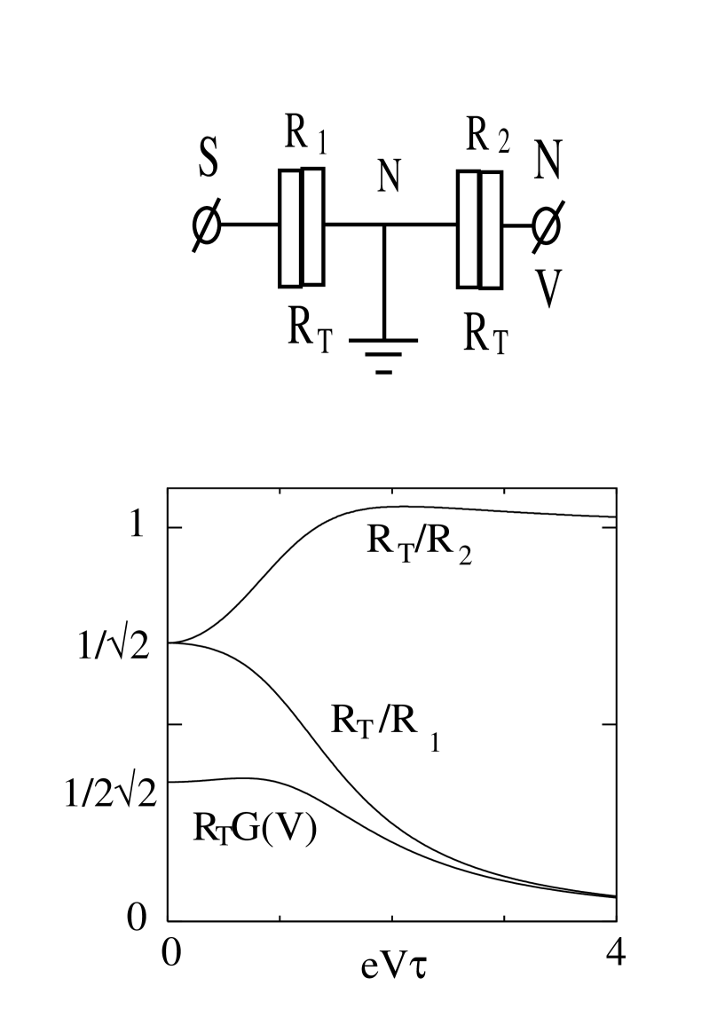
FIG. 1.: Double tunnel junction in circuit theory. Connection to the ground represents the leakage current. Effective conductances of both junctions along with the net conductance are plotted versus voltage applied.

- [1] M. Tinkham, Introduction to superconductivity, (McGraw-Hill, New York, 1996).
- [2] A. I. Larkin and Yu. V. Ovchinninkov, Sov. Phys. JETP 41,960 (1975).
- [3] A. I. Larkin and Yu. V. Ovchinnikov, Sov. Phys. JETP 46, 155 (1977).
- [4] G. E. Blonder, M. Tinkham and T. M. Klapwijk, Phys. Rev. B 25, 4515.
- [5] A. V. Zaitsev, Sov. Phys. JETP 59, 1163 (1984).
- [6] M. Yu. Kuprianov and V. F. Lukichev, Sov. Phys. JETP 67, 1163 (1988).
- [7] A. F. Volkov, A. V. Zaitsev, and T. M. Klapwijk, Physica C 210, 21 (1993).
- [8] Yu. V. Nazarov, Phys. Rev. Lett. 73, 1420 (1994).
- [9] C.W.J. Beenakker,in:Mesoscopic Quantum Physics, edited by E. Akkermans, G. Montambaux, J.-L. Pichard, and J.Zinn-Justin (North-Holland, Amsterdam, 1995).
- [10] C. W. J. Beenakker, Rev.Mod.Phys. 69, 731 (1997).
- [11] N. Argaman, Europhys. Lett. 38, 231 (1997).
- [12] S. Guéron, Ph. D. Thesis, Université Paris 6,1997.
- [13] S. G. den Hartog, B. J. van Wees, Yu. V. Nazarov, and T. M. Klapwijk, Phys. Rev. Lett. 79, 3250 (1997); S. G. den Hartog, B. J. van Wees, T. M. Klapwijk, Yu. V. Nazarov, and G. Borghs, Phys. Rev. B 56, 13738(1997).
- [14] C. W. J. Beenakker, Phys. Rev. B 51, 13883 (1995).
- [15] A. D. Stone, P. A. Mello, K. A. Muttalib, and J.-L. Pichard, in : Mesospopic Phenomena in Solids, edited by B. L. Altshuler, P. A. Lee, and R. A. Webb.
- [16] V. T. Petrashov, V. N. Antonov, P. Delsing and T. Claeson, Phys. Rev. Lett. 74, 5268 (1995).