[

Universality of electron correlations in conducting carbon nanotubes

Abstract

Effective low-energy Hamiltonian of interacting electrons in conducting single-wall carbon nanotubes with arbitrary chirality is derived from the microscopic lattice model. The parameters of the Hamiltonian show very weak dependence on the chiral angle, which makes the low energy properties of conducting chiral nanotubes universal. The strongest Mott-like electron instability at half filling is investigated within the self-consistent harmonic approximation. The energy gaps occur in all modes of elementary excitations and estimate at $0.01-0.1$ eV.

]

Single wall carbon nanotubes (SWNTs) are linear macromolecules whose individual properties can be studied by methods of nanophysics [1]. Recent demonstration of electron transport through single [2] and multiple [3] SWNTs has been followed by remarkable observations of atomic structure [4, 7], one-dimensional van Hove singularities [4], standing electron waves [8] and, possibly, electron correlations [9] in these systems. Moreover, the first prototype of a functional device - the nanotube field effect transistor working at room temperature - has been fabricated recently [10].

Structurally uniform SWNTs can be characterized by the wrapping vector $\vec{w}=N_{1}\vec{a}_{1}+N_{2}\vec{a}_{2}$ given by the linear combination of primitive lattice vectors $\vec{a}_{\pm}=(\pm 1,\sqrt{3})a/2$, with $a\approx 0.246$ nm (Fig. 1). It is natural to separate non-chiral armchair ($N_{1}=N_{2}$) and zig-zag ($N_{1}=-N_{2}$) nanotubes from their chiral counterparts. Recent scanning tunneling microscopy study [4] has revealed that individual SWNTs are generally chiral. According to the single-particle model, the nanotubes with $N_{1}-N_{2}=0$ mod $3$ have gapless energy spectrum [5] and are therefore conducting; otherwise, the energy spectrum is gapped and SWNTs are insulating. Therefore, on the level of non-interacting electrons, physical properties of SWNTs are determined by their geometry.

The Coulomb interaction in one-dimensional SWNTs should result in a variety of correlation effects due to the non-Fermi liquid ground state of the system. In particular, metallic armchair SWNTs are predicted to be Mott insulating at half-filling [11],[12],[13],[14]. Upon doping the nanotubes become conducting but still display density wave instabilities in three modes of elementary excitations with neutral total charge [15],[14].

Experimental observation of electron correlations still remains challenging since their signatures are usually masked by charging effects. Two recent transport spectroscopy experiments on an individual conducting SWNT [9] and a rope of SWNTs [16] produced contradicting results. The data by Tans et. al. [9] assumes spin polarized tunneling into a nanotube, which in turn suggests the interpretation in terms of electron correlations. On the other hand, the data by Cobden et. al. [16] fits the constant interaction model remarkably well and shows no signatures of exotic correlation effects. Since the atomic structure of particular SWNTs studied in these experiments is not known, it might be appealing to interpret the discrepancy in the results in terms of geometry-dependent many-particle properties of conducting SWNTs.

Unfortunately, consistent theory of interacting electrons in chiral SWNTs is lacking, despite such a theory has been recently developed for armchair nanotubes [15],[13],[14],[17]. In this work we establish effective low-energy model for conducting chiral SWNTs and evaluate its parameters (scattering amplitudes) from the microscopic theory. We found very weak dependence of the dominant scattering amplitudes on the chiral angle. This allows us to introduce universal low-energy Hamiltonian of conducting SWNTs. According to the results of the renormalization group analysis [14] the strongest Mott-like electron instability occurs at half-filling. We investigate this instability using the self-consistent harmonic approximation. Substantial energy gaps are found in all modes of elementary excitations. The conditions for experimental observation of the gaps are briefly discussed.

We start from the standard kinetic term $H_{k}$ of the tight-binding Hamiltonian for $p_{z}$ electrons of a graphite sheet [18],

$$H_{k}=\sum_{s,\vec{k}}\left\{\xi(\vec{k})a_{-,s}^{\dagger}(\vec{k})a_{+,s}(\vec{k})+h.c.\right\}.$$ (1)

Here $a_{p,s}(\vec{k})$ are the Fermi operators for electrons at the sublattice $p=\pm$ (Fig. 1) with the spin $s=\pm$ and the wavevector $\vec{k}=(k_{x},k_{y})$. The matrix elements are given by $\xi(\vec{k})=-t({\rm e}^{-{\rm i}k_{y}a/\sqrt{3}}+2{\rm e}^{{\rm i}k_{y}a/2\sqrt{3}}\cos k_{x}a/2)$, $t$ being the hopping amplitude between neighboring atoms. The eigenvalues of the Hamiltonian vanish at two Fermi points of the Brillouin zone, $\alpha\vec{K}$ with $\alpha=\pm$ and $\vec{K}=(K,0)$, $K=4\pi/3a$.

We consider conducting chiral $(N_{1},N_{2})$ SWNT of the radius $R=(a/2\pi)\sqrt{N_{1}^{2}+N_{1}N_{2}+N_{2}^{2}}$ whose axis $x^{\prime}$ forms the angle $\chi=\arctan[(N_{2}-N_{1})/\sqrt{3}(N_{1}+N_{2})]$ with the direction of chains of carbon atoms ($x$ axis in Fig. 1). Expanding Eq. (1) near the Fermi points to the lowest order in $\vec{q}=\vec{k}-\alpha\vec{K}=q(\cos\chi,\sin\chi)$ and introducing slowly varying Fermi fields $\psi_{p\alpha s}(x^{\prime})=L^{-1/2}\sum_{q=2\pi n/L}e^{iqx^{\prime}}a_{p\alpha s}(\vec{q}+\alpha\vec{K})$, we obtain,

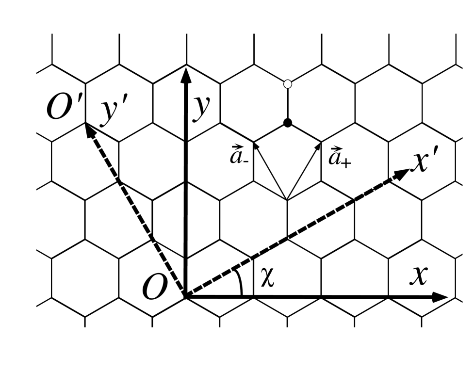
FIG. 1.: Graphite lattice consists of two atomic sublattices $p=+,-$ denoted by filled and open circles. SWNT at the angle $\chi$ to $x$ axis can be formed by wrapping the graphite sheet along $\vec{w}=OO^{\prime}$ vector.

$$H_{k}=-iv\sum_{p\alpha s}\alpha e^{-ip\alpha\chi}\int{\rm d}x^{\prime}\psi_{p\alpha s}^{\dagger}\partial_{x^{\prime}}\psi_{-p\alpha s},$$ (2)

with the Fermi velocity $v=\sqrt{3}ta/2\approx 8.1\times 10^{5}$ m/s. The kinetic term can be diagonalized by the unitary transformation

$$\psi_{p\alpha s}=\frac{1}{\sqrt{2}}e^{-ip\alpha\chi/2}\sum_{r=\pm}(r\alpha)^{\frac{1-p}{2}}\varphi_{r\alpha s}$$ (3)

to the basis $\varphi_{r\alpha s}$ of left- ($r=-$) and right- ($r=+$) movers.

The Coulomb interaction has the form

$$H_{int} = \frac{1}{2}\sum_{pp^{\prime},\left\{\alpha_{i}\right\},ss^{\prime}}V_{pp^{\prime}}(2\bar{\alpha}K)$$ (5)

$$\times\int dx^{\prime}\psi_{p\alpha_{1}s}^{\dagger}\psi_{p^{\prime}\alpha_{2}s^{\prime}}^{\dagger}\psi_{p^{\prime}\alpha_{3}s^{\prime}}\psi_{p\alpha_{4}s},$$

with the matrix elements

$$V_{pp^{\prime}}(2\bar{\alpha}K)=\frac{1}{\rho}\sum_{\vec{r}_{p}}U(\vec{r}_{p}-\vec{r}_{p^{\prime}})\exp[-2i\bar{\alpha}\vec{K}(\vec{r}_{p}-\vec{r}_{p^{\prime}})],$$ (6)

corresponding to the amplitudes of intra- ($p=p^{\prime}$) and inter- ($p=-p^{\prime}$) sublattice forward ($\bar{\alpha}=0$) and backward ($\bar{\alpha}=\pm 1$) scattering [19] (the sum is taken over the nodes of the sublattice $p$ of SWNT). Here $U(\vec{r})={e^{2}}/\{\kappa\sqrt{a_{0}^{2}+(x^{\prime})^{2}+4R^{2}\sin^{2}(y^{\prime}/2R)}\}$ is the Coulomb interaction with a short-distance cutoff $a_{0}\sim a$, $\rho=4\pi R/\sqrt{3}a^{2}$ is a linear density of sublattice nodes along SWNT, and $\bar{\alpha}=(\alpha_{1}-\alpha_{4})/2=(\alpha_{3}-\alpha_{2})/2$. We will choose the parameter $a_{0}$ from the requirement that the on-site interaction in the original tight-binding model corresponds to the difference between the ionization potential and electron affinity of $sp^{2}$ hybridized carbon [20]. This procedure gives $a_{0}=0.526a$.

The forward scattering part $H_{F}$ [terms with $\bar{\alpha}=0$ in Eq. (5)] of the Hamiltonian $H_{int}$ can be separated into the Luttinger model-like term $H_{\rho}$ and the term $H_{f}$ related to the difference $\Delta V(0)={V}_{pp}(0)-{V}_{p-p}(0)$ between intra- and intersublattice amplitudes,

$$H_{\rho} = \frac{V_{pp}(0)}{2}\int{\rm d}x^{\prime}\rho^{2}(x^{\prime}),$$ (7)

$$H_{f} = -\frac{\Delta V(0)}{2}\sum_{p\alpha\alpha^{\prime}ss^{\prime}}\int{\rm d}x^{\prime}\psi_{p\alpha s}^{\dagger}\psi_{-p\alpha^{\prime}s^{\prime}}^{\dagger}\psi_{-p\alpha^{\prime}s^{\prime}}\psi_{p\alpha s},$$ (8)

where $\rho=\sum_{p\alpha s}\psi_{p\alpha s}^{\dagger}\psi_{p\alpha s}$ is the total electron density. The backscattering Hamiltonian $H_{B}$ [terms with $\bar{\alpha}=\pm 1$ in Eq. (5)] can be subdivided into the intrasublattice $H_{b}^{(+)}$ ($p=p^{\prime}$) and intersublattice $H_{b}^{(-)}$ ($p=-p^{\prime}$) parts.

The dominant contribution to the forward scattering amplitudes $V_{pp^{\prime}}(0)$ comes from the long range component of the Coulomb interaction, $V_{pp}(0)=(2e^{2}/\kappa)\ln(R_{s}/R)$, where $R_{s}\simeq\min(L,D)$ characterizes the screening of the interaction due to a finite length $L$ of the SWNT and/or the presence of metallic electrodes at a distance $D$ [13]. The forward scattering differential part $\Delta V(0)$ and the intrasublattice backscattering amplitude $V_{pp}(2K)$ can be estimated from Eq. (6) as follows, $\Delta V(0),V_{pp}(2K)$ $\sim ae^{2}/\kappa R$ (for $a_{0}\sim a$). Despite the amplitudes $\Delta V(0),V_{pp}(2K)$ are much smaller than $V_{pp}(0),$ they produce essentially non-Luttinger terms in the low-energy Hamiltonian which will be important in further analysis.

We evaluated the matrix elements (6) numerically for chiral SWNTs with radiuses $R$ in the range $2R/a=4-7$ ($2R/a=5.5$ for (10,10) SWNTs). We found that dimensionless amplitudes $2\pi\kappa R[\Delta V(0),V_{pp}(2K)]/ae^{2}$ show very weak dependence on the radius of SWNT and its chiral angle (see Table 1). The results are sensitive to the value of the cutoff parameter $a_{0}$.

The intersublattice backscattering amplitude $V_{p-p}(2K)$ is almost three orders of magnitude smaller than $\Delta V(0)$, $V_{pp}(2K)$. This is due to the $C_{3}$ symmetry of a graphite lattice, which leads to an exact cancellation of the terms (6) contributing to $V_{p-p}(2K)$ in the case of a plane graphite sheet. The matrix elements $V_{p-p}(2K)$ are generally complex due to asymmetry of effective 1D intersublattice interaction potential (the matrix elements are real for symmetric zig-zag and armchair SWNTs). Let us note that after the unitary transformation (3) of the Hamiltonian $H=H_{k}+H_{int}$, the chiral angle $\chi$ enters only to the intersublattice backscattering matrix elements [21]. Due to the smallness of these matrix elements, the low-energy properties of chiral SWNTs are expected to be virtually independent of the chiral angle.

$a_{0}/a$	$\Delta V(0)$	$V_{pp}(2K)$	$|V_{p-p}(2K)|$
$0.4$	$0.44265-0.44274$	$0.97060-0.97095$	$0.6-2.2\times 10^{-3}$
$0.526$	$0.17378-0.17395$	$0.53549-0.53561$	$0.5-1.6\times 10^{-3}$
$0.7$	$0.04880-0.04895$	$0.24778-0.24797$	$0.3-1.5\times 10^{-3}$

TABLE I.: Scattering amplitudes $\Delta V(0)$, $V_{pp}(2K)$, $V_{p-p}(2K)$ in units $ae^{2}/2\pi\kappa R$ for all chiral SWNTs with radiuses $R$ in the range $2R/a=4-7$.

Neglecting the intersublattice backscattering we arrive to the universal low-energy model of conducting SWNTs given by the Hamiltonian $H=H_{k}+H_{F}+H_{b}^{(+)}$. The latter can be bosonized along the lines of Refs. [15, 14]. We introduce bosonic representation of the Fermi fields,

$$\varphi_{r\alpha s}=\frac{\eta_{r\alpha s}}{\sqrt{2\pi\tilde{a}}}\exp\left[{\rm i}rq_{F}x^{\prime}+\frac{{\rm i}r}{2}\left\{\theta_{\alpha s}+r\phi_{\alpha s}\right\}\right],$$ (9)

and decompose the phase variables $\theta_{\alpha s},\phi_{\alpha s}$ into symmetric $\delta=+$ and antisymmetric $\delta=-$ modes of the charge $\rho$ and spin $\sigma$ excitations, $\theta_{\alpha s}=\theta_{\rho+}+s\theta_{\sigma+}+\alpha\theta_{\rho-}+\alpha s\theta_{\sigma-}$ and $\phi_{\alpha s}=\phi_{\rho+}+s\phi_{\sigma+}+\alpha\phi_{\rho-}+\alpha s\phi_{\sigma-}$. The bosonic fields satisfy the commutation relation, $[\theta_{j\delta}(x_{1}),\phi_{j^{\prime}\delta^{\prime}}(x_{2})]={\rm i}(\pi/2){\rm sign}(x_{1}-x_{2})\delta_{jj^{\prime}}\delta_{\delta\delta^{\prime}}$. The Majorana fermions $\eta_{r\alpha s}$ are introduced [15] to ensure correct anticommutation rules for different species $r,\alpha,s$ of electrons, and satisfy $[\eta_{r\alpha s},\eta_{r^{\prime}\alpha^{\prime}s^{\prime}}]_{+}=2\delta_{rr^{\prime}}\delta_{\alpha\alpha^{\prime}}\delta_{ss^{\prime}}$. The quantity $q_{F}=\pi n/4$ is related to the deviation $n$ of the average electron density from half-filling, and $\tilde{a}\sim a$ is the standard ultraviolet cutoff.

The universal low-energy Hamiltonian of conducting SWNTs has the following bosonized form,

$$H = \sum_{j=\rho,\sigma}\sum_{\delta=\pm}\frac{v_{j\delta}}{2\pi}\int{\rm d}x^{\prime}\left\{K_{j\delta}^{-1}(\partial_{x^{\prime}}\theta_{j\delta})^{2}+K_{j\delta}(\partial_{x^{\prime}}\phi_{j\delta})^{2}\right\}$$ (20)

$$+\frac{1}{2(\pi\tilde{a})^{2}}\int{\rm d}x^{\prime}\{[\Delta V(0)-V_{pp}(2K)]$$

$$[\cos(4q_{F}x^{\prime}+2\theta_{\rho+})\cos 2\theta_{\sigma+}-\cos 2\theta_{\rho-}\cos 2\theta_{\sigma-}]$$

$$-\Delta V(0)\cos(4q_{F}x^{\prime}+2\theta_{\rho+})\cos 2\theta_{\rho-}$$

$$+\Delta V(0)\cos(4q_{F}x^{\prime}+2\theta_{\rho+})\cos 2\theta_{\sigma-}$$

$$-{\Delta V(0)}\cos 2\theta_{\sigma+}\cos 2\theta_{\rho-}$$

$$+{\Delta V(0)}\cos 2\theta_{\sigma+}\cos 2\theta_{\sigma-}$$

$$-{V}_{pp}{(2K)}\cos(4q_{F}x^{\prime}+2\theta_{\rho+})\cos 2\phi_{\sigma-}$$

$$+{V}_{pp}{(2K)}\cos 2\theta_{\sigma+}\cos 2\phi_{\sigma-}$$

$$+{V}_{pp}{(2K)}\cos 2\theta_{\rho-}\cos 2\phi_{\sigma-}$$

$$+{V}_{pp}{(2K)}\cos 2\theta_{\sigma-}\cos 2\phi_{\sigma-}\},$$

$v_{j\delta}=v\sqrt{A_{j\delta}B_{j\delta}}$ and $K_{j\delta}=\sqrt{B_{j\delta}/A_{j\delta}}$ being the velocities of excitations and exponents for the modes $j,\delta$. The parameters $A_{j\delta}$, $B_{j\delta}$ are given by

$$A_{\rho+} = 1+\frac{4\bar{V}(0)}{\pi v}-\frac{\Delta V(0)}{4\pi v}-\frac{V_{pp}(2K)}{2\pi v},$$ (21)

$$A_{\nu\delta} = 1-\frac{\Delta V(0)}{4\pi v}-\delta\frac{V_{pp}(2K)}{2\pi v},$$ (22)

$$B_{\nu\delta} = 1+\frac{\Delta V(0)}{4\pi v}.$$ (23)

with $\bar{V}(0)=[V_{pp}(0)+V_{p-p}(0)]/2$.

Since $\bar{V}(0)/v\sim\ln(R_{s}/R)$ $\gg 1$ and $\Delta V(0)/v$, $V_{pp}(2K)/v\sim a/R$ $\ll 1$, the renormalization of the parameters $K_{j\delta}$, $v_{j\delta}$ by the Coulomb interaction is the strongest in $\rho+$ mode. Assuming $\kappa=1.4$ [15] and $R_{s}=100$ nm we obtain $K_{\rho+}\simeq 0.2,v_{\rho+}\simeq v/K_{\rho+}$ for generic SWNTs with $R\sim 0.7$ nm [13]. The interaction in the other modes is weak: $v_{j\delta}=v,$ $K_{j\delta}=1,$ up to a factor $1+O(a/R).$

The renormalization group analysis of armchair SWNTs with long range Coulomb interaction has been performed in Refs. [14],[13]. The modification of the parameters of the Hamiltonian (20) by the neglected small term $V_{p-p}(2K)$ should not change the results qualitatively [22]. The most relevant perturbation is the umklapp scattering at half-filling. In this case the non-linear terms of the Hamiltonian (20), which do not contain $\cos 2\theta_{\sigma-}$ scale to strong coupling and the phases $\theta_{\rho+},\theta_{\sigma+},\theta_{\rho-},\phi_{\sigma-}$ get locked at $(\theta_{\rho+}^{(m)},\theta_{\sigma+}^{(m)},\theta_{\rho-}^{(m)},\phi_{\sigma-}^{(m)})=(0,0,0,0)$ or $(\pi/2,\pi/2,\pi/2,\pi/2)$. Therefore, the ground state of half-filled SWNT is the Mott insulator with all kinds of the excitations gapped.

To estimate the gaps quantitatively, we will employ the self-consistent harmonic approximation which follows from Feynman’s variational principle [23]. We consider trial harmonic Hamiltonian of the form:

$$H_{0}=\sum_{j\delta}\frac{v_{j\delta}}{2\pi}\int{\rm d}x^{\prime} \{ K_{j\delta}^{-1}[(\partial_{x^{\prime}}\theta_{j\delta})^{2}+(1-\delta_{j\sigma}\delta_{\delta-})q_{j\delta}^{2}\theta_{j\delta}^{2}]$$ (24)

$$+ K_{j\delta}[(\partial_{x^{\prime}}\phi_{j\delta})^{2}+\delta_{j\sigma}\delta_{\delta-}q_{j\delta}^{2}\phi_{j\delta}^{2}]\},$$ (25)

$q_{j\delta}$ being variational parameters. By minimizing the upper estimate for the Free energy $F^{*}=F_{0}+\left\langle H-H_{0}\right\rangle_{0}$ [23] one obtains the following self-consistent equations,

$$q_{\rho+}^{2} = \frac{2K_{\rho+}}{\pi\tilde{a}^{2}v_{\rho+}}c_{\rho+}\left\{[V_{pp}(2K)-\Delta V(0)]c_{\sigma+}\right.$$ (27)

$$\left.+\Delta V(0)c_{\rho-}+V_{pp}(2K)d_{\sigma-}\right\},$$

$$q_{\rho-}^{2} = \frac{2K_{\rho-}}{\pi\tilde{a}^{2}v_{\rho-}}c_{\rho-}\left\{\Delta V(0)c_{\rho+}+\Delta V(0)c_{\sigma+}\right.$$ (29)

$$\left.-V_{pp}(2K)d_{\sigma-}\right\},$$

$$q_{\sigma+}^{2} = \frac{2K_{\sigma+}}{\pi\tilde{a}^{2}v_{\sigma+}}c_{\sigma+}\left\{[V_{pp}(2K)-\Delta V(0)]c_{\rho+}\right.$$ (31)

$$\left.+\Delta V(0)c_{\rho-}-V_{pp}(2K)d_{\sigma-}\right\},$$

$$q_{\sigma-}^{2} = \frac{2}{\pi\tilde{a}^{2}K_{\sigma-}v_{\sigma-}}d_{\sigma-}V_{pp}(2K)\left\{c_{\rho+}-c_{\sigma+}-c_{\rho-}\right\},$$ (32)

where $c_{j\delta}=\left\langle\cos 2\theta_{j\delta}\right\rangle_{0}=\cos 2\theta_{j\delta}^{(m)}(\gamma\tilde{a}q_{j\delta})^{K_{j\delta}}$, $d_{\sigma-}=\left\langle\cos 2\phi_{\sigma-}\right\rangle_{0}=\cos 2\phi_{\sigma-}^{(m)}(\gamma\tilde{a}q_{\sigma-})^{1/K_{\sigma-}}$, $\left\langle...\right\rangle_{0}$ denotes averaging with respect to the trial Hamiltonian (25), and $\gamma\simeq 0.890$ for the exponential ultraviolet cutoff. Note that $\left\langle\cos 2\theta_{\sigma-}\right\rangle_{0}=0$, so that only the terms of the Hamiltonian (20) which scale to the strong coupling contribute to Eqs. (27)-(32).

In the limiting case of interest, $|\Delta V(0)|,|V_{pp}(2K)|\ll v$ and $K_{\rho+}\ll 1$, the solution of Eqs. (27)-(32) can be found in a closed form, giving rise to the following estimates for the gaps $\Delta_{j\delta}=v_{j\delta}q_{j\delta}$ in the energy spectra,

$$\Delta_{\rho+} = \frac{v_{\rho+}}{\gamma\tilde{a}}\left(\frac{2\gamma^{2}V_{\rho+}}{\pi v_{\rho+}}\right)^{1/(1-K_{\rho+})}$$ (33)

$$\Delta_{\rho-} = \frac{|\Delta V(0)|}{V_{\rho+}}\Delta_{\rho+}$$ (34)

$$\Delta_{\sigma+} = \frac{|V_{pp}(2K_{0})-\Delta V(0)|}{V_{\rho+}}\Delta_{\rho+}$$ (35)

$$\Delta_{\sigma-} = \frac{|V_{pp}(2K_{0})|}{V_{\rho+}}\Delta_{\rho+}$$ (36)

FIG. 2.: The energy gaps $\Delta_{j\delta}$ for the modes $\rho+$, $\sigma-$, $\sigma+$, $\rho-$ at $a_{0}=0.526a$ (lines marked by crosses, from top to bottom) and for the mode $\rho+$ at $a_{0}=0.4a$ (triangles) and at $a_{0}=0.7a$ (squares). The energy is in units $\hbar v/\tilde{a}\simeq 2.16$ eV for $\tilde{a}=a$.

with $V_{\rho+}=\left\{[\Delta V(0)-V_{pp}(2K)]^{2}+[\Delta V(0)]^{2}\right.$ $\left.+[V_{pp}(2K)]^{2}\right\}^{1/2}$. In the above expressions we used the approximation, $v_{0}/v_{\rho+}=K_{\rho+}$ and $v_{0}/v_{j\delta}=K_{j\delta}=1$ for $\sigma\pm$ and $\rho-$ modes. The formulae (33)-(36) indicate that the largest gap occurs in $\rho+$ mode, albeit all four gaps are of the same order for realistic values of the matrix elements (see Table 1). The gaps decrease as $\Delta_{j\delta}\propto(1/R)^{1/(1-K_{\rho+})}\simeq(1/R)^{5/4}$ with the tube radius. This should be contrasted to the $1/R$ dependence of wide semiconductor gaps and $1/R^{2}$ dependence of narrow deformation induced gaps [6] expected from the single particle picture.

In Figure 2 we present numerical results for the gaps $\Delta_{j\delta}$ for the cutoff parameter $a_{0}=0.526a$. The data for somewhat larger and somewhat smaller values of $a_{0}$ indicate possible variation of the gap $\Delta_{\rho+}$ due to uncertainty in the short distance cutoff of the Coulomb interaction. The gaps can be loosely estimated at $\Delta_{j\delta}\sim 0.01-0.1$ eV for typical SWNTs with $R\simeq 0.7$ nm. Due to the gaps in the spectrum of bosonic elementary excitations, the electronic density of states should disappear in the subgap region and display features at the gap frequencies and their harmonics. Both signatures should be observable by means of the tunneling spectroscopy.

Why have the gaps not been observed in the experiments [9, 16, 4]? This might be due to the effect of metallic electrodes. The difference in the workfunctions of the electrodes (Au, Pt) and the nanotube results in a downward shift of the Fermi level of the nanotube by a few tenths of an eV [4]. This causes substantial deviation $\Delta n=4q_{F}/\pi\sim 1$ nm^-1 of the electron density in SWNT from half filling, at least in the vicinity of the electrodes. Therefore, we expect the gap features to be observable in the layouts with well separated (to a distance $d\gg\hbar v_{F}/\Delta_{\rho+}$) source and drain contacts. The piece of nanotube between them should be well isolated from any conductor.

In conclusion, we have developed effective low-energy theory of conducting chiral SWNTs with the long-range Coulomb interaction. The many-particle properties of SWNTs are found to be virtually independent of the chiral angle. The universal Hamiltonian (20) of conducting SWNTs is introduced. The Mott-like energy gaps in the range of $0.01-0.1$ eV should be observable at half filling.

The authors would like to thank B.L. Altshuler, G.E.W. Bauer, R. Egger, Yu.V. Nazarov, and N. Wingreen for stimulating discussions. The financial support of the Royal Dutch Academy of Sciences (KNAW) is gratefully acknowledged. One of us (A.O.) acknowledges the kind hospitality at the NEC Research Institute.

REFERENCES

• [1] A. Thess et. al., Science, 273, 483 (1996).
• [2] S.J. Tans, et. al., Nature 386, 474, (1997).
• [3] M. Bockrath, et. al., Science, 275, 1922 (1997).
• [4] J.W.G. Wildöer, et. al., Nature 391, 59 (1998).
• [5] We do not discuss here the minigaps due to the curvature of the nanotube surface, see Ref. [6].
• [6] C.L. Kane, E.J. Mele, Phys. Rev. Lett. 78, 1932 (1997).
• [7] W. Clauss, D. J. Bergeron, A. T. Johnson, Phys. Rev. B 58, R4266 (1998).
• [8] L.C. Venema, et. al., submitted to Science.
• [9] S.J. Tans, M.H. Devoret, R.J.A. Groeneveld, and C. Dekker, Nature 394, 761 (1998).
• [10] S.J. Tans, A.R.M. Verschueren, and C. Dekker, Nature 393, 49 (1998).
• [11] L. Balents and M. P. A. Fisher, Phys. Rev. B 55, R11973 (1997).
• [12] Yu. A. Krotov, D.-H. Lee, and Steven G. Louie, Phys. Rev. Lett. 78, 4245 (1997).
• [13] C. Kane, L. Balents and M. P. A. Fisher, Phys. Rev. Lett. 79, 5086 (1997).
• [14] H. Yoshioka and A.A. Odintsov, to be published in Phys. Rev. Lett., preprint cond-mat/9805106.
• [15] R. Egger and A. O. Gogolin, Phys. Rev. Lett. 79, 5082 (1997).
• [16] D.H. Cobden, et. al., Phys. Rev. Lett. 81, 681 (1998).
• [17] Drawbacks of the analysis [15] are discussed in Ref. [14].
• [18] P. R. Wallace, Phys. Rev. 71, 622 (1947).
• [19] This definition is different from conventional one since it involves the Fermi points rather than the directions of motion of scatterred electrons.
• [20] see e.g. E. Moore, B. Gherman, and D. Yaron, J. Chem. Phys. 106, 4216 (1997).
• [21] The transformed matrix elements $V_{p-p}(2\bar{\alpha}K)e^{2i\bar{\alpha}p\chi}$ are invariant under $\pi n/3$ rotations in chiral angle $\chi_{n}=\chi_{0}+\pi n/3$, which correspond to equivalent representations of a nanotube.
• [22] We have checked this explicitly for (10,10) SWNTs at half filling and away from it.
• [23] R.P. Feynman, Statistical mechanics, Reading, Mass., W.A. Benjamin, Inc., 1972.