Coupling between Electron Spin and Ferromagnetic Clusters

Abstract

We analyze the adiabatic magnetization of ferromagnetic clusters in an intermediate coupling regime, where the anisotropic potential is comparable to other energy scales. We find a non-monotonic behavior of the magnetic susceptibility as a function of coupling with a peak. Coriolis coupling effects are calculated for the first time; they reduce the susceptibility somewhat.

I Introduction

Magnetic properties of a wide variety of ferromagnetic clusters, e.g. Fe, Ni and Co in transition metals involving 3d electrons [1, 2, 5, 6], and Ru, Rh and Pd associated with 4d electrons [3, 4, 5], are studied using the Stern-Gerlach technique. The observed deflection profile, caused by the interaction of magnetization and the gradient of field strength, provides information about these intrinsic magnetic moment of the cluster as well as its coupling to the other degrees of freedom in clusters. The size of cluster is small enough to be regarded as a single domain system, and the electrons involved form a single giant magnetic moment; we will call it the super-electron spin in this paper. It is quite interesting to see that, in such a low dimensional system, some elements form ferromagnetic clusters, even though the bulk material is nonmagnetic. Also, the magnetization is strongly dependent on the number of atoms in the clusters. Therefore, it is important in the present stage of study to establish a method of analysis for extracting the intrinsic magnetic moment from the observed deflection profile, and this is the motivation for the present work.

Let us consider the experimental set-up. First, the clusters formed by the laser evaporation, are cooled by the helium gas, and then the clusters are expanded to form a molecular beam. There is a problem in identifying the temperature experimentally. In the present study we assume that the clusters are in thermal equilibrium. The density of clusters in beam is low, so that the clusters may be assumed to be isolated beyond the equilibration zone. Therefore each cluster stays in a certain quantum state in the beam. Finally, the clusters enter into Stern-Gerlach magnet and are deflected by the interaction of the gradient of magnetic field and the magnetic polarization of super-spin induced by the magnetic field. At the entrance of the magnet, strength of the field changes gradually in time, and a time dependent interaction for the super-electron spin causes a transion of the initial quantum state to other quantum states. If the time dependence is sufficiently weak compared with coupling of the spin to other modes, the transition probability to other modes can be neglected. This is called the adiabatic approximation. In the present work, we calculate the profile and the magnetization with this assumption.

If the electrons were completely decoupled from other degrees of freedom such as rotational motion, the deflection profile would be a flat horizontal distribution independent of the field strength. But this is not actually the case for the observed profiles. A small coupling of the magnetic moment to internal coordinates of the cluster gives rise to spin relaxation, making the profile different from the flat distribution. Hence it is important to make clear how various couplings produce observed deflection profiles.

The simplest model is superparamagnetism in which the population of the magnetic states are proportional to a Boltzmann factor [7]. In other words, the cluster rotation plays a role as a heat bath for the super-electron spin in the magnetic field. In practical analysis for extracting the giant magnetic moment, the Langevin formula is widely employed. It assumes equilibrium with a thermal reservoir at a temperature which is the same as the source of the cluster beam. However, it predicts a rather sharp deflection profiles which is quite different from the broad profile that are often observed. Hence, the superparamagnetic model seems to be too simple for the analysis of the experiments.

Another simple model is locked-spin model in which the super-electron spin is frozen to the intrinsic orientation of the cluster, which of course is free to rotate [8, 9, 10]. This model seems successful in reproducing the small peak observed near zero deflection angle, which experimentalists call “superparamagnetism”. But it is applicable only to Gd clusters and not general. Furthermore, the model ignores the angular momentum of the super-electron spin, which is known to give recoil effects in the Einstein-de Haas effect.

We propose an intermediate coupling model as a method to extract the giant magnetic moment from the deflection profile [10]. This model covers the superparamagnetic and locked-moments models as weak and strong coupling limits, respectively. This paper is organized as follows: the intermediate model is explained and formulated in Sec. 2, numerical results of profiles and magnetization are presented for various strength of coupling, strength of magnetic field and temperature in Sec. 3. The conclusions and discussions are presented in Sec. 4.

II Intermediate Coupling Model

In the present model it is supposed that all the electron spins are aligned in the same direction through the exchange interaction. Thus, the electron spins are in stretched coupling states having a giant total spin $S=n_{s}N$, where $n_{s}$ is the number of spins participating the magnetic moment an atom. Since the magnetic moment is proportional to the total spin, the cluster has a single giant magnetic moment expressed as $\mu=g_{\rm s}S$, in terms of electronic gyromagnetic ratio $g_{\rm s}$.

Consider as a typical case the Fe₁₀₀ cluster at temperature 100K . This has a spin value of $S\simeq 100$ and a thermal rotational angular momentum $R\simeq 600$ in units of $\hbar$. These large values of $S$ and $R$ justify a classical treatment of the problem. In fact, in a previous paper [9] the classical treatment allowed the problem to be reduced a simple and transparent calculation.

this was examined for a simple case, by utilizing adiabatic invariance which makes the calculation easy and transparent.

However in a more general case, in which a fluctuation of spin orientation with respect to the cluster is significant, we are unable to make a simple classical treatment. Furthermore, in the classical treatment, the spin angular momentum is ignored, and thus angular momentum conservation is violated. Since this is a doubtful approximation when $S$ is comparable to $R$, we follow a fully quantum mechanical treatment.

Our Hamiltonian $H$ is expressed as sum of three terms

$$H=H_{\rm rot}+H_{\rm coupl}+H_{\rm mag},$$ (1)

where the terms are defined as follows. The first term, $H_{\rm rot}$, stands for the rotational energy of the cluster which is expressed as

$$H_{\rm rot}=\sum_{i=1}^{3}\frac{\hat{R}_{i}^{2}}{2{\cal J}_{i}},$$ (2)

where $\hat{R}_{i}$’s represent operators of three angular momentum components referred to the body fixed frame, and ${\cal J}_{i}$’s express principal moments of inertia. The vibrational modes are not taken into account, because the Debye-temperature, (for instance, 500[K] for iron) is much higher than the source temperature. In other words, the rotational motion is considered to work mainly as heat bath in the spin relaxation.

The second term, $H_{\rm coupl}$, expresses a coupling potential between the cluster and the super-electron spin, which is originated from the crystal magnetic anisotropy energy caused by molecular or crystal fields. The simplest form of the energy is the uniaxial magnetic anisotropy which, has already been examined in ref [10]. Here we assume that the clusters have an internal cubic structure and the potential has cubic symmetry. This is true for observation of the direction of easy magnetization being [100],[010] and [001] for iron and nickel. The anisotropy constant is measured in the form

$$E_{\alpha}=K_{1}(\alpha_{1}^{2}\alpha_{2}^{2}+\alpha_{2}^{2}\alpha_{3}^{2}+\alpha_{3}^{2}\alpha_{1}^{2})+K_{2}\alpha_{1}^{2}\alpha_{2}^{2}\alpha_{3}^{2}+\cdots$$ (3)

where $\alpha_{i}^{2}$’s express the direction cosines of super-electron spin. The measured values in the bulk are $K_{1}=36$ [mK/atom] and $K_{2}=13$ [mK/atom] for iron, and $K_{1}=-4$ [mK/atom] and $K_{2}=0$ [mK/atom] for nickel. We consider only the first term in the present calculation. In order to formulate the anisotropic interaction, let us start with the above classical picture for angular momentum variables, in which $S^{\prime}_{i}$’s commute.

$$H_{\rm coupl} = 8uS^{\prime\,4}(\alpha_{1}^{2}\alpha_{2}^{2}+\alpha_{2}^{2}\alpha_{3}^{2}+\alpha_{3}^{2}\alpha_{1}^{2}-\frac{1}{5})$$ (4)

$$= -u\left\{S^{\prime 4}_{1}+S^{\prime 4}_{2}+S^{\prime 4}_{3}-6(S^{\prime 2}_{1}S^{\prime 2}_{2}+S^{\prime 2}_{2}S^{\prime 2}_{3}+S^{\prime 2}_{3}S^{\prime 2}_{1})\right.$$ (6)

$$\left.+\frac{3}{5}(S^{\prime 2}_{1}+S^{\prime 2}_{2}+S^{\prime 2}_{3})^{2}\right\}$$

$$= -uS^{\prime 4}\sqrt{\frac{32}{35}}\left\{C^{(4)}_{4}(\hat{\mbox{\boldmath$S$}})+C^{(4)}_{-4}(\hat{\mbox{\boldmath$S$}})+\sqrt{\frac{14}{5}}C^{(4)}_{0}(\hat{\mbox{\boldmath$S$}})\right\},$$ (7)

Here $C_{\mu}^{(\lambda)}(\hat{\mbox{\boldmath$S$}})$ stands for the spherical harmonic proportional to $Y_{\lambda\mu}(\hat{\mbox{\boldmath$S$}})$; $S^{\prime}_{i}$ is the spin component with respect to the three axes in the body-fixed frame, $S_{i}$ denotes the spin component referred to the laboratory system, and $u=2K_{1}/n_{s}^{4}N^{3}$. The electron spin prefers the direction of 4-fold axes of the cubic symmetry. When the direction of the spin is along the 4-fold axes, the value of $H_{\rm coupl}$ has minimum energy $-\frac{8}{5}uS^{\prime 4}$. And when the direction of the spin is along the eight axes of $(\pm\frac{1}{\sqrt{3}}\pm\frac{1}{\sqrt{3}}\pm\frac{1}{\sqrt{3}})$ represented by body-fixed coordinate, the value of $H_{\rm coupl}$ turns out to be energy maximum $\frac{16}{15}uS^{\prime 4}$. In quantum Hamiltonian, $S^{\prime}$ are operators and we are interested in their matrix elements. The reduced matrix element obtained through the Wigner-Eckart theorem is expressed by

$$\langle S_{0}||\left[\hat{S}\right]^{L}||S_{0}\rangle=\left(\frac{1}{2}\right)^{L}\sqrt{\frac{(2S_{0}+L+1)!}{(2S_{0}-L)!}}.$$ (8)

For example, for $L=1$, one obtains the familiar form $\sqrt{S_{0}(S_{0}+1)(2S_{0}+1)}$. The interaction between the rotor and the super-electron spin in Eq. (4) is given by

$$H_{\rm coupl}(\mbox{\boldmath$S$},\Omega)=\sum_{\kappa,m}\left[S^{4}\right]^{4}_{m}{\cal D}^{4\ast}_{m\kappa}(\Omega)A_{\kappa},$$ (9)

where $\kappa$ takes the values of only 0 and $\pm 4$ and $A_{\pm 4}=\sqrt{5/14}A_{0}=-u\sqrt{32/35}$. The wave function of rotor can be expanded in terms of the ${\cal D}$-functions [13],

$$\phi_{R\mu}(\Omega)=\sum_{k}f_{Rk}{\cal D}^{R}_{\mu k}(\Omega).$$ (10)

Since the Hamiltonian $H_{\rm coupl}$ is scalar, the total angular momentum $\mbox{\boldmath$I$}=\mbox{\boldmath$R$}+\mbox{\boldmath$S$}$ is still a good quantum number for the first two terms of the Hamiltonians, $H_{\rm rot}+H_{\rm coupl}$. Accordingly, we select the base labeled by total angular momentum, and magnetic quantum number $I_{z}$. The basis is obtained by angular momentum coupling of the $\cal D$-function ${\cal D}^{R}_{\mu k}(\Omega)$ and $|S\sigma\rangle$ to $|IM\rangle$. Therefore, the total wave function of the rotor coupled with the super-electron spin is expressed as

$$\Psi_{\nu IM}=\sum_{Rk\sigma}\left\langle R\mu S\sigma|IM\right\rangle{\cal D}^{R}_{\mu k}(\Omega)f^{\nu I}_{Rk}\left|S\sigma\right\rangle,$$ (11)

where $\nu$ represents an index specifying states having the same $IM$. The matrix element of the coupling term between the bases in Eq. (11) is estimated as

$$(H_{\rm coupl})^{I}_{Rk,R^{\prime}k^{\prime}} = \sqrt{(2R+1)(2S+1)}(-1)^{S+R^{\prime}-I}$$ (13)

$$A_{\kappa}^{\prime}\left\langle Rk4\kappa|R^{\prime}k^{\prime}\right\rangle W(RSR^{\prime}S;I4),$$

where $\sqrt{2S_{0}+1}A_{\kappa}^{\prime}=A_{\kappa}\langle S_{0}||\left[\hat{S}\right]^{4}||S_{0}\rangle$. In our calculation we use potential strength parameter $u^{\prime}=A^{\prime}_{\pm 4}$. Now, the wave function (11) and the energy in the source are determined by diagonalizing $H_{\rm rot}+H_{\rm coupl}$. Since there remains the $(2I+1)$-fold degeneracy in energy for $M$, we may omit $M$ from the label for the energy $E_{\nu I}$.

The third term in Eq. (1) represents the interaction between an external magnetic field and the moments of the super-electron spin

$$H_{\rm mag}=-\mbox{\boldmath$B$}\cdot\mbox{\boldmath$\mu$}=-Bg_{\rm s}\hat{S_{z}},$$ (14)

We choose the direction of the applied magnetic field as the axis of quantization ($z$-axis). This interaction breaks rotational symmetry for the cluster, but the magnetic quantum number $M$ defined above is still conserved due to the choice of quantization axis. From (11) and (14), the matrix elements between two states are calculated as

$$\left\langle\Psi_{\nu IM}|H_{\rm mag}|\Psi_{\nu^{\prime}I^{\prime}M}\right\rangle=-Bg_{\rm s}\sqrt{2I^{\prime}+1}(-1)^{I^{\prime}}\left\langle I^{\prime}M10|IM\right\rangle h_{\nu I\nu^{\prime}I^{\prime}},$$ (15)

where $M$ independent part $h_{\nu I\nu^{\prime}I^{\prime}}$ is expressed as

$$h_{\nu I\nu^{\prime}I^{\prime}}=\sum_{Rk}f^{\nu I\ast}_{Rk}f^{\nu^{\prime}I^{\prime}}_{Rk}\sqrt{S(S+1)(2S+1)}(-1)^{R-S+1}W(ISI^{\prime}S;R1).$$ (16)

For simplicity, we set the moment of inertia around the intrinsic axes to take the same value

$${\cal J}_{1}={\cal J}_{2}={\cal J}_{3}={\cal J}.$$

In this case, total wave functions are classified by an additional quantum number $\pi_{k}=0,1,2,3$ ($k$ mod 4), since $H_{\rm rot}$ is diagonal and $H_{\rm coupl}$ couples to only the states having $k$-quantum numbers different by 4. This point is different from uniaxial anisotropy, in which $k$-quantum number is strictly conserved due to the axial symmetry. The total wave functions in the magnetic field are expressed as

$$\left|\Phi_{\alpha\pi_{k}M}(B)\right\rangle=\sum_{\nu I}F^{\nu I}_{\alpha\pi_{k}M}(B)\left|\Psi_{\nu I\pi_{k}M}\right\rangle,$$ (17)

where $\alpha$ labels state in the same $\pi_{k},M$.

To compare with the experiment, we calculate the average magnetization, which we regard as the ensemble average of $\langle S_{z}\rangle$. This is the sum of the product of the expectation value of $S_{z}$ and the occupation probability of each state. Now we proceed ahead with the important assumption that effect of the magnetic field is adiabatic when the cluster passes through Stern-Gerlach magnet. As variation of the magnetic field is slow when the cluster enters into and goes out from Stern-Gerlach magnet. Firstly the clusters are retained in the source region. In this region, as the cluster ensemble is in thermal equilibrium, the occupation probability of each quantum state is proportional to the Boltzmann factor $\exp(-E_{\nu I\pi_{k}}/k_{\rm B}T)$.

The magnetization of each state in Eq. (17) is calculated as

$$S_{z,\alpha(\nu I)\pi_{k}M}(B)=\langle\Phi_{\alpha(\nu I)\pi_{k}M}\mid\hat{S}_{z}\mid\Phi_{\alpha(\nu I)\pi_{k}M}\rangle,$$ (18)

where $\alpha(\nu I)$ stands for the label of states connected adiabatically with the states $(\nu I)$ defined in absence of the magnetic field.

Under the adiabatic condition, any transition between energy levels does not occur even if magnetic field is applied. Occupation probability of each quantum state is not altered during the flight. Then the deflection profile is obtained by

$$P(s,B,T)=\frac{1}{Z(T)}\sum_{\nu I\pi_{k}M}\delta(s-S_{z,\alpha(\nu I)\pi_{k}M})\exp\left(\frac{-E_{\nu I\pi_{k}}}{k_{\rm B}T}\right)$$ (19)

where $Z(T)$ represents partition function given by

$$Z(T)=\sum_{\nu I\pi_{k}}(2I+1)\exp\left(\frac{-E_{\nu I\pi_{k}}}{k_{\rm B}T}\right).$$ (20)

The magnetization, the ensemble average $\langle S_{z}\rangle_{\rm en.av.}$, is expressed by

$$\langle S_{z}\rangle_{\rm en.av.}=\frac{1}{Z(T)}\sum_{\nu I\pi_{k}M}\left\langle\Psi_{\alpha(\nu I)\pi_{k}M}\mid S_{z}\mid\Psi_{\alpha(\nu I)\pi_{k}M}\right\rangle\exp\left(\frac{-E_{\nu I\pi_{k}}}{k_{\rm B}T}\right).$$ (21)

III Magnetic Susceptibility

In almost all the Stern-Gerlach experiments with clusters the magnetic field is so weak that the magnetization shows linear dependence. Hence, it is important in the analysis of the experiment to estimate the magnetic susceptibility. Besides, the magnetic susceptibility for the superparamagnetism and locked moment model has a well-known value; to examine the magnetic susceptibility will give us how intermediate coupling model describes the two extreme model. Therefore, we calculate the magnetic susceptibility for intermediate coupling model and discuss weak and strong coupling limit in the following subsections.

For the present, let us discuss the general expression of magnetic susceptibility. Using Feynman theorem, we obtain the expectation value of $S_{z}$ as

$$\left\langle\hat{S_{z}}\right\rangle=-\left\langle\frac{\partial}{\partial(Bg_{\rm s})}H_{\rm mag}\right\rangle\\ =-\frac{\partial}{\partial(Bg_{\rm s})}\left\langle H_{\rm mag}\right\rangle.$$ (22)

The magnetic susceptibility is expressed as

$$\chi = \left.\frac{\partial}{\partial g_{\rm s}B}\left\langle\hat{S_{z}}\right\rangle_{\rm en.av.}\right|_{Bg_{S}=0}=-\left.\frac{\partial^{2}}{\partial(Bg_{\rm s})^{2}}\Delta E_{\rm en.av.}\right|_{Bg_{\rm s}=0}$$ (23)

$$= -\frac{2}{Z}\sum_{\nu IM}\sum_{\nu^{\prime}I^{\prime}}\frac{|\langle\Psi_{\nu^{\prime}I^{\prime}M}|\hat{S_{\rm z}}|\Psi_{\nu IM}\rangle|^{2}}{E_{\nu I}-E_{\nu^{\prime}I^{\prime}}}$$ (24)

where $\Delta E_{\rm en.av.}$ and $Z$ means the ensemble average of energy shift and partiation function, respectively.

We will deal with a certain limit of susceptibility (24) in the following two subsections. Strong coupling limit will be discussed in Subsect. III A. The weak coupling limit will be treated in Subsect. III B. Susceptibility in intermediate coupling will be calculated numerically in Subsect. III C.

A Susceptibility for Strong Coupling

We first consider the energy eigenvalue and the eigenstate of $H_{\rm rot}+H_{\rm coupl}$ in the strong coupling limit. The angular momentum of the rotor $R$ is mixed, while total angular momentum $I$ and the $z$-component of total angular momentum, $M$ are conserved in the absence of the magnetic field. We rewrite the Hamiltonian of the present model in terms of the total angular momentum, $I$

$$\frac{\hat{\mbox{\boldmath$I$}}^{2}+\hat{\mbox{\boldmath$S^{\prime}$}}^{2}-2\hat{\mbox{\boldmath$I$}}\cdot\hat{\mbox{\boldmath$S^{\prime}$}}}{2{\cal J}}+H_{\rm coupl}(\hat{\mbox{\boldmath$S^{\prime}$}}).$$ (25)

The third term of the numerator is the Coriolis term, which couples the degrees of freedom of super-electron spin to one of the rotor. The Coriolis term is not taken into account in the locked moment model, because the super-electron spin is not included as a dynamical variable. On the other hand, it must be noticed that the intermediate coupling model includes the Coriolis term. As will be seen this term contributes to the magnetic susceptibility. Since $H_{\rm coupl}$ gives a dominant contribution to the energy eigenvalue of $H_{\rm rot}+H_{\rm coupl}$ in the strong coupling, we treat the Coriolis term as a perturbation. The coupling Hamiltonian $H_{\rm coupl}(\hat{\mbox{\boldmath$S^{\prime}$}})$ is written in terms of the intrinsic component only (see Eq. (7)). Then it is advantageous to select a direct product the eigenfunction of total angular momentum and its $z$-component and eigenfunction of super-electron spin with respect to intrinsic frame; ${\cal D}^{I}_{MK}(\Omega)\otimes\sum_{\sigma_{k}}g_{\sigma_{k}}|S\sigma_{k}\rangle$ as the basis. The energy eigenvalue of the Hamiltonian neglecting Coriolis term is

$$\frac{\hbar^{2}}{2{\cal J}}(I(I+1)+S(S+1))+u^{\prime}E^{\rm A}_{N},$$ (26)

where $u^{\prime}E^{\rm A}_{N}$ is the energy eigenvalue of the coupling $H_{\rm coupl}$. Without the Coriolis interaction, the energy spectra is of rotational band with band head energy $u^{\prime}E^{\rm A}_{N}$.

Let us now discuss the ground band of the present model in the strong coupling. Figure 1 illustrates the numerically evaluated energy eigenvalues of $H_{\rm coupl}$ in the space $|S\sigma\rangle$. The eigenstate of $H_{\rm coupl}$ must belong to a certain irreducible representation of the point group $O$. The irreducible representations $A_{1},E,T_{1}$ for $S=4n$, $A_{2},E,T_{2}$ for $S=4n+2$, and irreducible representations $T_{1},T_{2}$ for odd $S$ appear in the lowest energy region. Considering the dimension of these representations, namely 1,1,2,3 and 3 for $A_{1},A_{2},E,T_{1}$ and $T_{2}$ respectively, the bunch of the levels contain six states. The six fold and the eight fold approximately degenerate states appear at the lowest and highest energies, respectively. This fact implies that the direction of super-electron spin is localized to the six (eight) directions corresponding to the potential minima (maxima) in the lowest (the highest) bunching states for large $S$. Therefore, these states are approximated by

$$R^{i}|SS\rangle,$$ (27)

where $R^{i}$ stands for the operator corresponding to the rotation from 3rd axis to $i$th direction of the potential minima.

For the present, we shall take into account the Coriolis term in first-order perturbation theory. According to first order perturbation theory of degenerate states, we solve the secular equation to determine the energy shift and perturbed states. In this case, each level in the rotational band is $6(2I+1)^{2}$-fold degenerate: The quantum number $M,K$ have the values $-I\leq M~{}K\leq I$ and the ground state of super-electron spin is 6-fold degenerate. The dimension of the secular equation is decreased by a factor $(2I+1)$ because the motion under the total Hamiltonian conserves $M$. As we discussed before, the direction of super-electron spin corresponds to one of the potential minima for the ground state. We choose the direction of quantization axis as one of the potential minima. This selection of quantization axis yields the Coriolis matrix element as

$$\mbox{\boldmath$\hat{I}\cdot\hat{S}$}=\hat{I_{i}}\hat{S_{i}}+(\hat{I_{+}^{i}}\hat{S_{-}^{i}}+\hat{I_{-}^{i}}\hat{S_{+}^{i}})$$ (28)

$$\hat{I_{i}}=R^{i}\hat{I_{3}}R^{i\dagger},\quad\hat{I_{\pm}^{i}}=R^{i}\hat{I_{\pm}}R^{i\dagger},$$ (29)

$$\hat{S_{i}}=R^{i}\hat{S_{3}}R^{i\dagger},\quad\hat{S_{\pm}^{i}}=R^{i}\hat{S_{\pm}}R^{i\dagger}.$$ (30)

Only the first term of Eq. (28) is involved in the calculation of the matrix element of Coriolis term between the parallel direction of super-electron spin. The second terms do not contribute the Coriolis matrix element between parallel or antiparallel direction but orthogonal direction. Actually, we can estimate the matrix element of raising and lowering operators of super-electron spin

$$\langle SS|\hat{S_{\pm}}R^{\prime}(\theta)|SS\rangle=\cases{0,&\quad\mbox{for $\theta=0$}\cr\propto\hbar\sqrt{2S}(1/2)^{S+1},&\quad\mbox{for $\theta=\frac{\pi}{2}$}\cr 0,&\quad\mbox{for $\theta=\pi$}\cr}$$ (31)

where $R^{\prime}(\theta)$ is the rotation through angle $\theta$ around the axis perpendicular to the 3 axis. We find from Eq. (31) that the second term of the Coriolis term ( Eq. (28)) is vanishingly small for large super-electron spin. This allows us to approximate the Coriolis term as

$$\hat{\mbox{\boldmath$I$}}\cdot\hat{\mbox{\boldmath$S$}}\simeq\hat{I_{i}}\hat{S_{i}}.$$ (32)

We can solve the secular equation for approximated Coriolis term, Eq. (32), for each degenerate rotational state. The wave function results in the eigenstate of $I^{i}$;

$$|IMN\xi\rangle=|IMKi\rangle=R^{i}|SS\rangle R^{i}\sqrt{\frac{2I+1}{8\pi^{2}}}{\cal D}^{I}_{MK}(\Omega)\quad(N\leq 6).$$ (33)

where $\xi$ specifies the energy levels split by the Coriolis term. For the ground band $(N\leq 6)$, $\xi$ corresponds to $K$, and $N$ is labeled by the index of the direction of super-electron spin $i$. The first order energy shift is obtained as

$$\langle I^{\prime}MK^{\prime}j|2\hat{\mbox{\boldmath$I$}}\cdot\hat{\mbox{\boldmath$S$}}|IMKi\rangle=2\hbar^{2}KS\delta_{K,K^{\prime}}.$$ (34)

We neglect the coupling between ground band and excited band because the energy difference between these bands are large in the strong coupling. Higher order perturbation would take into account this coupling and would give the deviation from the locked moment due to the finite strength of coupling. But we do not discuss the deviation in this paper.

The energy eigenvalue of (25) is divided into three parts

$$E_{IMN\xi}=\frac{\hbar^{2}}{2{\cal J}}(I(I+1)+S(S+1))+u^{\prime}E^{\rm A}_{N}+\frac{\hbar^{2}}{2{\cal J}}E_{N\xi}^{\rm C}$$ (35)

where $E^{\rm C}_{N\xi}$ is the energy shift by the perturbation of the Coriolis term and is equal to Eq. (34) for the ground band ($N\leq 6$)

The susceptibility is evaluated through Eq. (24) as

$$\chi = -\frac{2}{Z}\sum_{IMN\xi}\sum_{I^{\prime}N^{\prime}\xi^{\prime}}\frac{|\langle I^{\prime}MN^{\prime}\xi^{\prime}|\hat{S_{z}}|IMN\xi\rangle|^{2}}{\frac{\hbar^{2}(I(I+1)-I^{\prime}(I^{\prime}+1))}{2{\cal J}}-\frac{\hbar^{2}(E^{\rm C}_{N\xi}-E^{\rm C}_{N^{\prime}\xi^{\prime}})}{2{\cal J}}-u^{\prime}(E^{\rm A}_{N}-E^{\rm A}_{N^{\prime}})}\exp\left(-\frac{E_{IMN\xi}}{k_{\rm B}T}\right).$$ (36)

For the single rotational band with $(2I+1)^{2}$ fold degeneracy, levels of which the angular momentum are larger than $I_{\rm c}(T)=\sqrt{6.2{\cal J}k_{\rm B}T/\hbar^{2}}$ contributes only less than 10 percent of the partition function. We call $I_{\rm c}(T)$ cut-off angular momentum. When the band head of excited bands are much larger than the energy of the cut-off level, that is,

$$u^{\prime}(E^{\rm A}_{N}-E^{\rm A}_{1})\gg\frac{\hbar^{2}\{I_{\rm c}(T)\}^{2}}{2{\cal J}},\quad(N\geq 7)$$ (38)

the higher bands do not have considerable occupation probabilities. Therefore, it is possible to describe the susceptibility with the ground band only. Substituting energy of the ground band obtained through the Eqs. (34) and (35) and the matrix element of $\hat{S_{z}}$ evaluated by the wave function of the ground band Eq. (33) into Eq. (LABEL:bare_su), we get

$$\chi = -\frac{1}{Z}\sum_{IMKi}\sum_{I^{\prime}Ki^{\prime}}4{\cal J}\frac{\delta_{ii^{\prime}}S^{2}\frac{2I+1}{2I^{\prime}+1}|\langle IM10|I^{\prime}M\rangle|^{2}|\langle IK10|I^{\prime}K\rangle|^{2}}{I(I+1)-I^{\prime}(I^{\prime}+1)}$$ (40)

$$\hskip 170.71652pt\times\exp\left(-\frac{\frac{\hbar^{2}(I(I+1)+S(S+1)+2KS)}{2{\cal J}}+uE^{\rm A}_{i}}{k_{\rm B}T}\right).$$

This is different from the susceptibility for locked moment [8] only in the Coriolis term. Since the average angular momentum is about $I\simeq 600$, one can safely evaluate Eq. (40), treating $I,K$ as a continuous variable and replacing the sum by an integral. Thus we get

$$\chi = \frac{2{\cal J}}{3}\left(1-\frac{e^{-\beta S^{2}}}{S}\int_{0}^{S}e^{\beta t^{2}}dt\right)=\sum_{n=0}^{\infty}\frac{2{\cal J}}{3\hbar^{2}}\frac{(-1)^{n}2^{n}}{(2n+3)!!}(\beta S^{2})^{n+1}$$ (41)

$$= \frac{2}{9}\frac{\hbar^{2}S^{2}}{k_{\rm B}T}\left(1-\frac{2}{5}\frac{\hbar^{2}S^{2}}{2{\cal J}k_{\rm B}T}+\frac{4}{35}\left(\frac{\hbar^{2}S^{2}}{2{\cal J}k_{\rm B}T}\right)^{2}+\cdots\right)<\frac{2}{9}\frac{\hbar^{2}S^{2}}{k_{\rm B}T},$$ (42)

where $\beta=\frac{\hbar^{2}}{2{\cal J}k_{\rm B}T}$. The leading order is the same as the locked moment susceptibility. The higher orders mean the correlation by the Coriolis term; in other words, a recoil effect due to the angular momentum of the super-electron spin, or Einstein-de Haas effect. We find from Eq. (42) that this effect reduces the magnetic susceptibility compared with one of the locked moment. This fact will be substantial in numerical calculation in Subsect. III C. We close this subsection with evaluating the condition of neglecting the recoil effect. For finite temperature, the cluster is excited by the thermal rotational excitation. For the rotational band with $(2I+1)^{2}$-fold degeneracy, the most major population of angular momentum is $I_{\rm eff}(T)=\sqrt{\frac{2{\cal J}k_{\rm B}T}{\hbar^{2}}}$. Therefore, the typical energy splitting by the Coriolis coupling becomes $\hbar^{2}\frac{SI_{\rm eff}(T)}{{\cal J}}$. We can neglect the recoil effect under the high temperature condition

$$k_{\rm B}T\gg\frac{\hbar^{2}SI_{\rm eff}(T)}{{\cal J}}.$$ (43)

B Susceptibility for Weak Coupling

In this subsection we discuss the susceptibility for the weak coupling and high temperature limits. Firstly we discuss the energy eigenvalue and the eigenfunction of $H_{\rm rot}+H_{\rm coupl}$ in the weak coupling. The angular momentum of rotor $R$ is approximately conserved due to the weak coupling. In the absence of coupling, the energy eigenvalue is a single rotational band with $(2R+1)^{2}$ fold degeneracy. The coupling removes the degeneracy; the first order energy shift is determined by solving the secular equation in degenerate space. Therefore, the energy eigenvalue is described as $\frac{\hbar^{2}R(R+1)}{2{\cal J}}+\Delta E_{I\lambda(R)}$ where $\lambda(R)$ specifies states adiabatically connected with $R$, and $\Delta E_{I\lambda(R)}$ stands for the eigenvalue of the weak anisotropic coupling. The unperturbed base is expressed by

$$|IMRk\rangle=\sum_{\mu\sigma}\langle R\mu S\sigma|IM\rangle{\cal D}_{\mu k}^{R}|S\sigma\rangle$$ (44)

The coupling is treated as the first order perturbation to degenerate states. The perturbed wavefunction is expressed as

$$\Psi_{\lambda(R)IM}=\sum_{k\sigma}\left\langle R\mu S\sigma|IM\right\rangle{\cal D}^{R}_{\mu k}(\Omega)c^{\lambda(R)}_{k}\left|S\sigma\right\rangle,$$ (45)

where the coefficient $c^{\lambda(R)}_{k}$ is determined by the diagonalization of $H_{\rm coupl}$ in each degenerate rotational level.

Now we evaluate the magnetic susceptibility for weak coupling by employing the Eq. (24). Equation (24) reduces the calculation of magnetic susceptibility to the evaluation of second order energy shift. The energy denominator between different $R$ levels are much larger than the one of the same $R$ in the weak coupling. So, we neglect the contribution from different $R$ in the perturbation. The orthogonality condition $\sum_{k}c^{\lambda(R)\ast}_{k}c^{\lambda^{\prime}(R)}_{k}=\delta_{\lambda\lambda^{\prime}}$ yields the matrix element of Zeeman interaction between the weak coupling base, Eq. (45), as

$$\left\langle\Psi_{\lambda(R)IM}|\hat{S_{z}}|\Psi_{\lambda^{\prime}(R)I^{\prime}M}\right\rangle = \delta_{\lambda,\lambda^{\prime}}\sqrt{2I^{\prime}+1}(-1)^{I^{\prime}}\left\langle I^{\prime}M10|IM\right\rangle$$ (47)

$$\times\sqrt{S(S+1)(2S+1)}(-1)^{R-S+1}W(ISI^{\prime}S;R1).$$

Under the approximation, Eq. (24) becomes

$$\chi=-\frac{2}{Z}\sum_{R}\left(\sum_{\lambda(R)MI\neq I^{\prime}}\frac{|\left\langle\Psi_{\lambda(R)IM}|\hat{S_{z}}|\Psi_{\lambda(R)I^{\prime}M}\right\rangle|^{2}}{\Delta E_{I\lambda(R)}-\Delta E_{I^{\prime}\lambda(R)}}e^{-\frac{E_{R}+\Delta E_{I^{\prime}\lambda(R)}}{k_{\rm B}T}}\right),\quad E_{R}=-\frac{\hbar^{2}R(R+1)}{2{\cal J}}.$$ (48)

Since $\Delta E_{I^{\prime}\lambda(R)}$ is small because of the weak coupling, we can expand $e^{-\frac{\Delta E_{I^{\prime}\lambda(R)}}{k_{\rm B}T}}$ up to first order as $1-\frac{\Delta E_{I^{\prime}\lambda(R)}}{k_{\rm B}T}$. Rearranging the summention, we get

$$\chi=-\frac{2}{Z}\sum_{R}\left(\sum_{\lambda(R)MI>I^{\prime}}\frac{|\left\langle\Psi_{\lambda(R)IM}|\hat{S_{\rm z}}|\Psi_{\lambda^{\prime}(R)I^{\prime}M}\right\rangle|^{2}}{k_{\rm B}T}\right)e^{-\frac{E_{R}}{k_{\rm B}T}}.$$ (49)

Putting Eq. (47) into Eq. (49), and expanding for $R$, Therefore, we obtain the magnetic susceptibility

$$\chi = 2\frac{\sum_{R=0}^{\infty}\left(\frac{4S(S+1)(2S+1)R^{2}}{9}+O(R)\right)\exp\left(-\frac{\hbar^{2}R(R+1)}{2{\cal J}k_{\rm B}T}\right)}{\sum_{R=0}^{\infty}\left((2R+1)^{2}(2S+1)\right)\exp\left(-\frac{\hbar^{2}R(R+1)}{2{\cal J}k_{\rm B}T}\right)}$$ (50)

At high temperature limit many levels contribute to the summention over $R$. Therefore one can evaluate Eq. (50), treating $R$ as a continuous variable and replacing the sum by integral. Thus, we get

$$\chi=\frac{2S(S+1)}{9k_{\rm B}T}$$ (51)

It is observed in this subsection that the locked moment susceptibility is obtained in the weak coupling and high temperature limit. One should note that this does not mean the super-electron spin is locked in the weak coupling. In fact, taking into account the axial deformation, the susceptibility of weak and strong coupling becomes different. In the weak coupling, the energy level is dependent on the axial deformation through the $k$ quantum number:

$$E_{IMRk}=\frac{\hbar^{2}}{2{\cal J}_{1}}(R(R+1)-k^{2})+\frac{\hbar^{2}}{2{\cal J}_{3}}k^{2}.$$ (52)

The matrix element is independent of the deformation, because the Eq. (47) is independent of $\lambda$. Therefore, the leading order of $1/k_{\rm B}T$ expansion of magnetic susceptibility is deformation independent even if the energy is dependent on $k$, and is $2S(S+1)/9$ even in an axial deformed cluster. On the other hand, in strong coupling the energy level for the ground band expressed as

$$E_{IMK}=\frac{\hbar^{2}}{2{\cal J}_{1}}(I(I+1)-K^{2}+KS)+\frac{\hbar^{2}}{2{\cal J}_{1}}K^{2}$$ (53)

If we neglect the Coriolis term, this is the same as the one of the weak coupling, apart from the degeneracy. The matrix element for axial deformed cluster is not different even in the strong coupling. Hence, the magnetic susceptibility of the axial deformed cluster is same as Eq. (40) apart from the energy. Since the matrix element divided by the energy difference $I(I+1)-I^{\prime}(I^{\prime}+1)$ is dependent on the deformation, the magnetic susceptibility becomes deformation dependent. Therefore, considering the axial deformation, the susceptibility for the weak and strong coupling limits are different. The two limits happen to be the same value when the value of ${\cal J}_{i}^{\prime}s$ are equal. This equality does not mean the super-electron spin is locked in the weak coupling.

C Intermediate Coupling

We numerically calculate the magnetic susceptibility for intermediate coupling in this subsection. In numerical calculations of the deflection profile and the magnetization, a main task is diagonarization of Hamiltonian matrices of large dimensions. In the source area, the partial Hamiltonian $H_{\rm mag}$ is zero, and therefore the total angular momentum is conserved. The dimension of matrices to be diagonarized is approximately $S\times I_{\rm eff}(T)$. The dimension of matrices to be diagonarized is of the order of 10⁵. In the magnetic field where states having $I/2$ different are mixed, the number of dimension is magnified by $I/2$, and becomes eventually of the order of 10⁷. It may not be feasible in numerical calculations. Let us use a similarity transformation in order to scale down the angular momenta. In Eq. (13), the matrix element is approximated as

$$(H_{\rm coupl})_{RK,R^{\prime}K^{\prime}}\simeq A^{\prime}_{\kappa}\frac{\sqrt{(2R+1)(2R^{\prime}+1)}}{2\overline{R}+1}d_{\kappa\mu}^{4}(\theta_{1})d_{\mu 0}^{4}(\theta_{2})$$ (54)

with

$$\overline{R}=\frac{R+R^{\prime}}{2}~{}~{}~{}{\rm and}~{}~{}~{}\mu=R^{\prime}-R,$$ (55)

and two angles,$\theta_{1}$ and $\theta_{2}$, are defined respectively as

$$\cos\theta_{1} = \sqrt{\frac{\overline{K}}{\overline{R}}}~{}~{}~{}~{}{\rm with}~{}~{}~{}~{}\overline{K}=\frac{K+K^{\prime}}{2},$$ (56)

and

$$\cos\frac{\theta_{2}}{2} = \sqrt{\frac{(\overline{R}-S+I)(S-\overline{R}+I)}{4\overline{R}S}}.$$ (57)

These angles are invariant under a scale transformation defined as

$$\pmatrix{r,r^{\prime}~{}\overline{r}\cr k,k^{\prime}~{}\overline{k}\cr s,i,m\cr}=\eta\pmatrix{R,R^{\prime}~{}\overline{R}\cr K,K^{\prime}~{}\overline{K}\cr S,I,M\cr}.$$ (58)

In a similar manner, the matrix elements given in Eq. (15) are expressed approximately as

$$\left\langle\Psi_{\nu\pi_{K}IM}\mid H_{\rm mag}\mid\Psi_{\nu^{\prime}I^{\prime}\pi_{K}M}\right\rangle \simeq Bg_{\rm s}\sqrt{S(S+1)}\frac{\sqrt{(2I+1)(2I^{\prime}+1)}}{2\overline{I}}$$ (60)

$$\sum_{RK}f_{RK}^{\nu I*}f_{RK}^{\nu^{\prime}I^{\prime}}(-)^{I^{\prime}-I}d_{0\,I-I^{\prime}}^{1}(\theta_{3})d_{I-I^{\prime}\,0}^{1}(\theta_{4})$$

with

$$\cos\theta_{3} = \sqrt{\frac{M}{\overline{I}}}$$ (61)

$$\cos\frac{\theta_{4}}{2} = \sqrt{\frac{(\overline{I}-S+R)(S-\overline{I}+R)}{4\overline{I}S}}$$ (62)

The two additional angles, $\theta_{3}$ and $\theta_{4}$ are also invariant under the scale transformation. Eventually these four angles are invariant with respect to the scale transformation in Eq. (58). The four $d$-functions are all smooth functions of the four angles.

In the numerical calculation we scale down the super-electron spin quantum number $S$. To make $\hat{S}^{2}$ invariant under the similarity transformation, Eq. (58), the Plank constant is changed according to $\eta$. In other words, we can scale down the angular momentum quantum number by adjusting Plank constant as

$$\hbar^{\prime}=\frac{\hbar}{\eta},~{}~{}~{}s=\eta S.$$ (63)

The temperature $k_{\rm B}T$, coupling $u^{\prime}$, and magnetic field parameter $g_{\rm s}B\hbar S$, which have dimension of energy, are invariant under the similarity transformation. In the following, the unit of these energy parameter is selected as $\frac{\hbar^{2}S^{2}}{2{\cal J}}$ which is also invariant under the similarity transformation.

In the numerical calculation, we set the cut off of super-spin $s=S_{\rm c}$ and the cut off of total angular momentum $I_{\rm max}$. $\eta$ is decided through the $S_{\rm c}$ and Eq. (63) as $\eta=S_{\rm c}/S$.

We are now ready to calculate numerically the susceptibility for intermediate coupling. It is already known by the analysis in the above two subsections that the susceptibility becomes the locked moment in the limits. To achieve locked moment limit, the ground state of the $H_{\rm coupl}$ has to be approximately six fold degenerate. When we diagonalize $H_{\rm coupl}$ in $S_{\rm c}=10$ (see Fig. 1) three energy levels having 1-fold, 3-fold, and 2-fold degeneracy from lower energy to higher make a bunch around the ground state. The energy differences of these states are about 0.01. In contrast to this, we find from Fig. 1 that the energy difference between bunch of the ground state and the first excited bunch is about 1.0. The energy spacing between six states around the ground states are much smaller than the energy spacing between the ground bunch and the first excited bunch. Therefore, it seems reasonable that the ground state is approximately 6-fold degenerate for $S_{\rm c}=10$.

A truncation of the angular momentum is necessitated due to computational limitations. We select $I_{\rm max}=80$ in the calculation. As mentioned previously, we do not confident about the calculation of partition function out of the reliable range of temperature. Hence, the numerical calculation of partition function is reliable only $I_{\rm c}(T)\leq I_{\rm max}$. This restricts the range of temperature as $k_{\rm B}T<20.6$. We choose $20$ for the temperature.

We display the magnetic susceptibility of our calculation in Fig. 2. The first point to be discussed is whether our calculation reaches the two distinct limits discussed above. If the coupling is much smaller than the temperature, the susceptibility decreases and converges to $2/9$. Therefore our calculation agrees with the analysis for weak coupling discussed in Subsect. III B.

Let us discuss the strong coupling limit. In Subsect. III A we discuss the condition of temperature and coupling in which the susceptibility attains the locked moment value. The condition for the coupling and for the temperature are expressed in Eq. (38) and Eq. (43), respectively. These two conditions for $S_{\rm c}=10$ become;

$$\frac{u^{\prime}}{k_{\rm B}T}\gg 3.1,~{}~{}{\rm and}~{}~{}k_{\rm B}T\gg 4.$$ (64)

Therefore, we can regard $\frac{u}{k_{\rm B}T}\simeq 9$ for $k_{\rm B}T=20$ as the strong coupling region. However, in Fig. 2, the susceptibility is not $2/9$ even if the coupling becomes larger than 9. In particular, one might not readily believe that the susceptibility is smaller than $2/9$. One should recall that we evaluate the strong coupling limit of susceptibility including the effect of Coriolis coupling as Eq. (42). We find from this expression that the susceptibility is decreased by the recoil effect. We calculate the susceptibility for $k_{\rm B}T=20$ through Eq. (42). The result is illustrated in Fig. 2 and is close to the numerically computed susceptibility. Nevertheless, the numerically computed susceptibility shows some deviation from the value of Eq. (42). A possible reason for this is that the quantum fluctuation between different potential minima of the coupling decreases the susceptibility.

We find a peak at $\frac{u^{\prime}}{k_{B}T}=0.55$ in Fig. 2. This peak is accounted that the energy splitting of anisotropic interaction $2u^{\prime}$ is comparable to the energy splitting by Coriolis term $\frac{\hbar^{2}}{2{\cal J}}4I_{\rm eff}S$. The width of energy splitting of anisotropic interaction corresponds to the energy difference between potential maxima and minima i.e. $\frac{8}{3}u^{\prime}$. In practice the width becomes smaller due to the quantum fluctuation and is found $2u^{\prime}$ for $S=10$ from Fig. 1. Then the peak is expected to be,

$$2u^{\prime}\simeq\frac{\hbar^{2}}{2{\cal J}}4I_{\rm eff}S~{}~{}\Leftrightarrow~{}~{}\frac{u^{\prime}}{k_{\rm B}T}\simeq 2\sqrt{\frac{\hbar^{2}S^{2}}{2{\cal J}}\frac{1}{k_{\rm B}T}}\simeq 0.45.$$ (65)

In fact, this condition is consistent with the observed position of peak.

Let us move to the next point. As mentioned in introduction, one often assumes the superparamagnetism, in which susceptibility is $\frac{1}{3}S(S+1)$, for the clusters to analyze the experiments. From Fig. 2 that the superparamagnetic limit is not reach in any range of coupling strength.

The last point is the temperature dependence of the magnetization. It is reasonable to consider that the susceptibility decreases as the temperature increased because of thermal fluctuations. A quite opposite dependence is reported in Ref. [1]. However, our calculations does not show such a behavior in any range of coupling.

IV Profiles and Magnetization

As mentioned in the previous section, a truncation of the angular momentum is necessary due to the computational limitations. The procedure of calculating profile includes the large dimensional diagonalzation of Hamiltonian $H_{\rm mag}$. To make it practicable, we choose a truncated value of $I_{\rm max}=26$, and the magnitude of super-electron spin $S_{\rm c}=10$. As discussed in section III, this choice narrows the reliable range of temperature. The reliable range of temperature for this cut-off becomes $k_{\rm B}T<2$. Since high temperature is one of the conditions for the strong coupling limit, we should select as large temperature as possible. Eventually, we choose $k_{\rm B}T=2$ which is maximum for the reliable range of $I_{\rm max}=26$.

Firstly we pay attention to the magnetic field dependence of the deflection profile. Figure 3 shows the deflection profile for three different strengths of the magnetic field $g_{\rm s}B\hbar S=0.5,2,10$, respectively. Many experiments show that peak deflection is always to the strong field. Our calculation also exhibits deflection of a similar nature. By solving the classical equation of motion, De Heer et al. have demonstrated in Ref [11] that the coupling between super-spin and cluster body causes the deflection behavior. We will have a closer examination of this statement in terms of our quantal model.

In order to make our discussion transparent, we discuss the weak coupling limit first. We can see from Fig. 3 that the profile of the weak coupling is a flat but slightly sloping distribution in the weak magnetic field. Figure 4, which shows the energy levels of the weak coupling $u^{\prime}=4.47\times 10^{-3}$ for $S_{\rm c}=2,M=0,\pi_{k}=0$ and $R\simeq 3$ or $4$, helps us to understand the distribution in terms of the energy level. In the absence of magnetic field, the weak coupling removes 15-fold degeneracy of unperturbed rotational levels; Energy levels result in a bunch of states around the unperturbed rotational levels. The applied magnetic field further splits these levels, and rearranges each one more likely to be the eigenfunction of $S_{z}$, when the applied magnetic field becomes stronger than the coupling. In other words, the super-spin precesses about the direction of magnetic field independently from the cluster (decoupling) for $g_{\rm s}B\hbar S>u^{\prime}$. Although the magnetization increases proportional to the magnetic field before the decoupling, occupation probabilities of the same $R$ levels become almost equal because of the weak coupling. Then, the magnetization remains small and the profile becomes flat, rectangle like distribution. When the Zeeman splitting equals to the typical energy difference of the rotational levels: $2g_{\rm s}B\hbar S=2\hbar^{2}R_{\rm eff}/2{\cal J}$, the pseudo-crossing between different rotational levels occurs. To put it another way, the pseudo-crossing occurs where the Larmor precession frequency $\omega_{\rm L}$ is comparable to the cluster rotation frequency $\omega_{\rm rot}$; $\omega_{\rm L}\simeq\omega_{\rm rot}$. That is to say, the pseudo-crossing leads to exchange the occupation probabilities between those levels. Therefore, the magnetization increases and profile develops a peak at $\langle S_{z}\rangle/S=1$ like the Boltzmann distribution.

The above discussion leads us to divide the mechanism of magnetization into two types, that is, the magnetization by the process of decoupling and pseudo-crossing. When the coupling is weak, these two are separated definitely. This makes the magnetic field dependence of magnetization peculiar as shown in figure 5. The magnetization linearly increases as the magnetic field in the process to decoupling; then, remains steady by the decoupling of super-spin; finally, increases suddenly because of the pseudo-crossing. Since the magnetic field region of the decoupling and pseudo-crossing can not be divided into the intermediate and strong coupling, the peculiar behavior of magnetization disappears.

Let us now turn to the strong coupling. The calculated susceptibility (Fig 2) indicates that $u^{\prime}=11.2$ is in the strong coupling region. However, the calculated profile for $u^{\prime}=11.2$ in figure 3 is not identical with the locked moment profile. We attribute this to the Coriolis term, which is important at the temperature of our ensemble, $k_{\rm B}T=2$. A higher temperature was possible in the calculation in ref [10] because simpler anisotropy term there permitted smaller dimension Hamiltonian matrices.

Finally, let us move to the discussion of the profiles in intermediate coupling. We characterize the profiles by the cumulants. Since the cumulant higher than the second order vanishes for the Gaussian probability distribution, the characterization of the profiles by cumulant clearly shows us the deviation from Gaussian profile. In our calculation the third and the fourth order cumulants are much smaller than the first and the second one, so the Gaussian profile gives a reasonable description.

We now discuss the first (Fig. 7) and the second order cumulant (Fig. 8) in more detail. These correspond to ensemble average of the magnetization and width of the profile, respectively. We can estimate the second order cumulant of the locked moment profile in the absence of magnetic field and the rectangle profile as $\frac{1}{9}$ and $\frac{S(S+1)}{3S^{2}}$, respectively. The general trend of the first order cumulant looks like more or less one of either the superparamagnetic or locked moment. Although, we introduce the present model for describing the intermediate behavior between superparamagnetic and locked moment, the magnetization of intermediate coupling is smaller than one of the locked moment. This is because the Coriolis term decreases the susceptibility, as we discussed in Sec.III. We may note, in passing, that the anomalous behavior in the weak coupling, discussed earlier, should appear when the energy splitting by the magnetic field comparable to typical energy difference of rotational level, that is,

$$2g_{\rm s}B\hbar S\simeq\frac{2\hbar^{2}R_{\rm eff}}{2{\cal J}}~{}~{}\Leftrightarrow~{}~{}g_{\rm s}B\hbar S\simeq\frac{1}{S}\sqrt{\frac{\hbar^{2}S^{2}k_{\rm B}T}{2{\cal J}}}\simeq 0.14$$ (66)

But it is not seen in the figure 7.

The second order cumulant is sensitive to the coupling. The stronger the coupling becomes, the narrower the profile. The cut off angular momentum in this calculation is rather small than the perturbation. We calculate cumulant for higher temperature by applying the perturbation technique. Figure 6 shows the second order cumulant for $I_{\rm max}=80,k_{\rm B}T=20$ as the function of the coupling strength.

The second order cumulant becomes closer to the strong coupling limit $S^{2}/9$ around the coupling $u^{\prime}=3.5$. It decreases almost linearly in the region of the coupling beyond $20$ due to the tunneling between different direction of super-electron spin. Since the perturbation theory is valid for the magnetic field weaker than the coupling strength, the super-spin do not decouple from the cluster. Therefore, the profile is not the rectangle profile. We can estimate the second order cumulant of weak coupling limit. We find the magnetization of each level in this limit from the diagonal part of Eq. (47);

$$\langle S_{z}\rangle=\sqrt{2I+1}(-1)^{I}\left\langle IM10|IM\right\rangle\sqrt{S(S+1)(2S+1)}(-1)^{R-S+1}W(ISIS;R1).$$ (67)

The second order cumulant for weak coupling is estimated as

$$\langle S_{z}\rangle^{2}_{\rm cumulant} = \frac{S(S+1)(2S+1)}{Z}\sum_{RIM\lambda(R)}(2I+1)|\left\langle IM10|IM\right\rangle|^{2}|W(ISIS;R1)|^{2}\exp(-\frac{E_{R}}{k_{\rm B}T})$$ (68)

We treat $R$ as a continuous variable as in the Subsect. III A and get

$$\langle S_{z}\rangle^{2}_{\rm cumulant} \simeq \frac{1}{9}S(S+1)$$ (70)

Actually, in Fig. 6, the second order cumulant is not close to the one of the rectangle profile $1/3$, but close to $\frac{S_{\rm c}(S_{\rm c}+1)}{9S_{\rm c}^{2}}\simeq 0.122$.

To make the profile rectangle, the super-spin is decoupled from the cluster because of the strong magnetic field compare with the coupling;

$$g_{\rm s}B\hbar S\gg u^{\prime}.$$ (71)

Furthermore, pseudo-crossing do not occur at least for the levels having a typical angular momentum. Because, pseudo-crossing changes occupation probability of the levels.

$$g_{\rm s}B\hbar S<\frac{\hbar^{2}}{2{\cal J}}2R_{\rm eff}$$ (72)

However, in the perturbation for the magnetic field, the magnetic field is always smaller than the coupling. Hence, we can not describe the rectangle profile by perturbation for the coupling.

To describe the regime around the rectangle profile, we calculate magnetic field or coupling dependence of $\langle S_{z}\rangle^{2}$ by perturbation of the coupling under the two assumptions discussed above. The detailed account of calculation is presented in appendix. Here we give just the result Eq. (A21).

$$\langle S_{z}\rangle^{2} = \frac{1}{3}S(S+1)-\frac{8^{2}}{15\times 9^{2}}\left(\frac{u^{\prime}}{Bg_{\rm s}\hbar}\right)^{2}$$ (74)

$$+\left\{\frac{4}{9\times 15}\left(\frac{-190+39S(S+1)}{693}\right)-\frac{4}{15\times 9^{2}}S(S+1)\right\}\left(\frac{u^{\prime}}{k_{\rm B}T}\right)^{2}.$$

The higer order cumulant shows the deviation from the gaussian profile. As a detail of the calculated higher order cumulants from obtained profiles are not shown, the result is much smaller than the second order. When one analizes the experiment in more detail, the higher order cumulants may bring about important imformation.

For example, the third order cumulant (Fig. 9) characterizes asymmetry of the profile. In the whole range of magnetic field, the third order cumulant is smaller than the second order and is smaller as the coupling becomes stronger. The profiles are always symmetric with respect to $\langle S_{z}\rangle=0$ in the absence of magnetic field. When the magnetic field is applied, the asymmetry grows on account of the time reversal symmetry breaking. The third order cumulant have a peak at $g_{\rm s}B/k_{\rm B}T\simeq 2$. In the strong magnetic field, the profiles have a narrow peak at $\frac{\langle S_{z}\rangle}{S}=1$ like Fig. 3; The profiles are more likely to be symmetric but still not quite. In other words, the third order cumulant decreases but is not equal to zero.

V Conclusions and Discussion

Using an intermediate coupling model, we have studied the magnetization of ferromagnetic clusters in a Stern-Gerlach magnet. In this model the super-electron spin is free but couples to the cluster ions through an anisotropic potential. This model is expected to describe the intermediate behavior between the superparamegnetic and the locked moment. In evaluating the profiles or the magnetization, we assume that the variation of the magnetic field in entering the magnet is slow in time, i.e. adiabatic. Hence, any transition between the quantum states is suppressed; the occupation probability of each quantum state is determined in the source area where the magnetic field is absent.

We examined the magnetic susceptibility of the present model applying perturbation theory. Especially, the magnetic susceptibility in the strong and in weak coupling limits are discussed analytically. We expected the intermediate coupling model to approach the locked moment behavior in the strong coupling limit. However, there is a crucial difference between the strong coupling limit of the present model and the locked moment model. In the present model the super-electron spin degree of freedom is treated explicitly and the Coriolis term arises due to the conservation of total angular momentum, while in the locked moment model the Coriolis term is neglected. Consequently, the magnetic susceptibility is different from, and smaller than the locked moment. In the weak coupling limit, we expect the susceptibility of the present model to become superparamagnetic value. But the susceptibility in the present model obtained by the perturbation theory is not the superparamagnetic value in any range of the coupling.

We find that the irregular magnetic field response noticed in ref [10] also exists in the weak coupling region of the present model. The magnetization linearly increases before the decoupling; and is saturates after the decoupling. Then, once the pseudo-crossing between different $R$ levels occurs, the magnetization increases again. Before the decoupling, the susceptibility arises as a perturbation of the magnetic field. But after the decoupling, or once the pseudo-crossing takes place, the susceptibility becomes nonperturbative. Instead, we need to diagonalize the total Hamiltonian, which is difficult for today’s computers for high temperatures and large cut off angular momentum. In ref [10], one of the authers (GB) discussed the susceptibility after the decoupling using uniaxial coupling. They found that the susceptibility reaches the superparamagnetic value. Therefore, if we would calculate the susceptibility after the decoupling, the susceptibility would be superparamagnetic.

Although an anomalous temperature dependence is reported in ref [1], the calculated susceptibility is always positive. We do not reproduce the anomalous temperature dependence.

The “ superparamagnetic peak ” which is seen in the profile obtained by the locked moment model is not seen in the present calculation even in the strong coupling limit. As discussed before, the strong coupling limit of our model is different from the locked moment model due the Coriolis term. Hence, the effect of Coriolis term destroys the superparamagnetic peak. If we would be able to calculate in such high temperature that the Coriolis term can be negligible, the peak would appear in the deflection profile.

Finally, we summarize our method of analysis of the Stern-Gerlach deflection function. We calculated the cumulant of the profiles up to 3rd order to characterize the profiles. We found from figure 7 that the first and second order cumulants are dominant. In particular, the evaluation of the susceptibility and second order cumulant by the perturbation technique gave us the analytical expression of the second order cumulant and magnetic susceptibility for high temperature and strong or weak coupling. One can extract the magnetic moment and the coupling strength by fitting observed magnetic susceptibility and the second order cumulant into the calculated second order cumulant and the magnetic susceptibility.

VI Acknowledgment

Part of the calculations were performed with a computer VPP500 at RIKEN (Research Institute for Physical and Chemical Research, Japan) and SX4 at RCNP (Research Center of Nuclear Physics). The authors wish to thank Mr. M.Kaneda and Dr. A.Ansari for their helpful advice. We gratefully acknowledge helpful discussions with Dr. N.Tajima especially on the various coupling schemes. One of the authors (NH) would like to thank A. Bulgac for letting him participate to the program “Atomic Clusters” (INT-98-2). This work is finacially supported in part by the Grant-in-Aid for Finance Research (09640338).

A The second order cumulant for the decoupling regime

In this appendix we derive Eq. (74) under the assumption Eq. (71) and Eq. (72). The ensemble average of the second order cumulant determined through $\langle S_{z}\rangle^{2}$ of each level and the energy in the absence of magnetic field. Let us start the calculation of second order cumulant with evaluating $\langle S_{z}\rangle^{2}$. The assumption Eq. (71) assures us of applying perturbation theory of the coupling. Then we treat $H_{\rm coupl}$ as perturbative and $H_{\rm rot}+H_{\rm mag}$ as nonperturbative. The degeneracy remains for intrinsic quantum number $k$ when we select ${\cal D}^{R}_{\mu k}(\Omega)\otimes|S\sigma\rangle$ as unperturbed bases. According to perturbation theory for degenerate case, the unperturbed bases are obtained as eigenstates of the Hamiltonian $H_{\rm coupl}$ of the degenerate space;

$$\Psi^{(0)}_{RM\sigma\nu}=\sqrt{\frac{2R+1}{8\pi^{2}}}c_{\nu}^{k}{\cal D}^{R}_{\mu k}(\Omega)\otimes|S\sigma\rangle,~{}~{}~{}M=\mu+\sigma$$ (A1)

The effect of the coupling is included by first- and second-order perturbation theory. In the perturbed wave function, there exists mixing with different rotational states. Now we should recall the assumption Eq. (72) in which the energy difference between different rotational states are much larger than the magnetic field. This justifies that we can neglect the mixing with the different rotational states. Therefore, the perturbed wave function is evaluated as

$$\Psi^{(2)}_{RM\sigma\nu}=\left(1-\frac{1}{2}\sum_{\sigma\neq\sigma^{\prime}}\frac{u^{\prime 2}|(h_{\rm coupl})^{RM}_{\nu^{\prime}\sigma^{\prime},\nu\sigma}|^{2}}{\left\{Bg_{\rm s}\hbar(\sigma-\sigma^{\prime})\right\}^{2}}\right)\Psi^{(0)}_{R\sigma\nu M}$$ (A2)

$$+\sum_{\sigma\neq\sigma^{\prime}}\frac{u^{\prime}(h_{\rm coupl})^{RM}_{\nu\sigma^{\prime},\nu\sigma}}{Bg_{\rm s}\hbar(\sigma-\sigma^{\prime})}\Psi^{(0)}_{R\sigma^{\prime}\nu M}+\sum_{\sigma\neq\sigma^{\prime}}{\rm(Const.)}\Psi^{(0)}_{R\sigma^{\prime}\nu^{\prime}M}.$$ (A3)

with

$$u^{\prime}(h_{\rm coupl})^{RM}_{\nu^{\prime}\sigma^{\prime},\nu\sigma}=\langle\Psi^{(0)}_{R\sigma^{\prime}\nu^{\prime}M}|H_{\rm coupl}|\Psi^{(0)}_{R\sigma\nu M}\rangle=u^{\prime}\delta_{\nu,\nu^{\prime}}\Delta_{\nu R}\langle R\mu^{\prime}4m|R\mu\rangle\langle S\sigma 4m|S\sigma^{\prime}\rangle,$$ (A4)

where $\Delta_{\nu R}$ represents the eigenvalue of $h_{k,k^{\prime}}=\sum_{\kappa}\frac{A_{\kappa}}{A_{\pm}4}\langle Rk4\kappa|R^{\prime}k^{\prime}\rangle$ and $u^{\prime}=A_{\pm 4}\frac{\langle S||S^{4}||S\rangle}{\sqrt{2S+1}}$. Using the perturbed wave function Eq. (A3), we calculate $\langle S_{z}\rangle^{2}$ up to second order for the coupling,

$$\langle S_{z}\rangle^{2} = \sigma^{2}+\frac{u^{\prime 2}}{(Bg_{\rm s}\hbar)^{2}}C_{2},$$ (A6)

$$~{}~{}{\rm where}~{}~{}C_{2}=2\sigma\sum_{\sigma\neq\sigma^{\prime}}\frac{|(h_{\rm coupl})^{RM}_{\nu^{\prime}\sigma^{\prime},\nu\sigma}|^{2}}{(\sigma^{\prime}-\sigma)}.$$

Let us move on the evaluation of the energy in the absence of magnetic field. We should evaluate the energy which is adiabatically connected with state in the finite magnetic field. If the coupling is absent, the unperturbed wavefunction Eq. (A1) adiabatically connects between states in the magnetic field and one in the absence of magnetic field. Hence, we start from unperturbed wavefunction Eq. (A1), then introduce the coupling up to the second-order. According to the perturbation theory, the first order energy shift $u^{\prime}\epsilon^{(1)}_{\nu R}$ is evaluated the expectation value of $H_{\rm coupl}$ for unperturbed state;

$$u^{\prime}\epsilon^{(1)}_{\nu R}=\langle R\mu 40|R\mu\rangle\langle S\sigma 40|S\sigma\rangle u^{\prime}\Delta_{\nu R}.$$ (A7)

In the second order energy shift, different rotational states mix. However, as is mentioned above, the assumption Eq. (72) enables us to neglect the mixing of different rotational states. Therefore we neglect second order energy shift.

We are now able to calculate ensemble average of $\langle S_{z}\rangle^{2}$ using Eq. (A6) and Eq. (A7). Expanding not only $\langle S_{z}\rangle$ but also the Boltzmann factor up to second order, we get the ensemble average of $\langle S_{z}\rangle^{2}$ as

$$\langle S_{z}\rangle^{2}_{\rm en.av.} = \frac{\sum_{R\nu\sigma M}\left(\sigma^{2}+\left(\frac{u^{\prime}}{Bg_{\rm s}\hbar}\right)^{2}C_{2}+\cdots~{}\right)\exp\left(\frac{-E_{R}+u^{\prime}\epsilon^{(1)}_{\nu R}+\cdots}{k_{\rm B}T}\right)}{\sum_{R\nu\sigma M}\exp\left(\frac{-E_{R}+u^{\prime}\epsilon^{(1)}_{\nu R}+\cdots}{k_{\rm B}T}\right)}$$ (A8)

$$\simeq \frac{\sum_{R\nu\sigma M}\left[\sigma^{2}-\frac{u^{\prime}}{k_{\rm B}T}\sigma^{2}\epsilon^{(1)}_{\nu R}+\left\{\left(\frac{u^{\prime}}{Bg_{\rm s}\hbar}\right)^{2}C_{2}+\frac{1}{2}\left(\frac{u^{\prime}}{k_{\rm B}T}\right)^{2}\sigma^{2}{\epsilon^{(1)}_{\nu R}}^{2}+\cdots\right\}\right]\exp\left(\frac{-E_{R}}{k_{\rm B}T}\right)}{\sum_{R\nu\sigma M}\left\{1-\frac{u^{\prime}}{k_{\rm B}T}\epsilon^{(1)}_{\nu R}+\frac{1}{2}\left(\frac{u^{\prime}}{k_{\rm B}T}\right)^{2}{\epsilon^{(1)}_{\nu R}}^{2}+\cdots\right\}\exp\left(\frac{-E_{R}}{k_{\rm B}T}\right)}.$$ (A9)

$\sum_{\nu}\epsilon^{(1)}_{\nu R}=0$, $\sum_{\nu}\sigma^{2}\epsilon^{(1)}_{\nu R}=0$, because Tr $\Delta_{\nu R}=\sum_{\kappa}\langle Rk40|Rk\rangle=0$. Expanding Eq. (A9) up to second order of $u^{\prime}$, we get

$$\langle S_{z}\rangle^{2}_{\rm en.av.}=\frac{S(\sigma^{2})}{S(1)}+\frac{S(C_{2})}{S(1)}\left(\frac{u^{\prime}}{Bg_{\rm s}\hbar}\right)^{2}+\frac{1}{2}\left(\frac{S(\sigma^{2}{\epsilon_{\nu R}^{(1)}}^{2})}{S(1)}-\frac{S({\epsilon_{\nu R}^{(1)}}^{2})S(\sigma^{2})}{S(1)^{2}}\right)\left(\frac{u^{\prime}}{k_{\rm B}T}\right)^{2},$$ (A10)

where $S(x)$ is defined as

$$S(x)=\sum_{R\nu\sigma M}x\exp\left(-E_{R}/k_{\rm B}T\right).$$ (A11)

Let us estimate $S(x)$’s appearing in Eq. (A10).

$$S(1) = \sum_{R}(2S+1)(2R+1)^{2}\exp\left(\frac{-E_{R}}{k_{\rm B}T}\right).$$ (A12)

$$S(\sigma^{2}) = \sum_{R}\frac{1}{3}S(S+1)(2S+1)(2R+1)^{2}\exp\left(\frac{-E_{R}}{k_{\rm B}T}\right).$$ (A13)

Before calculating the other $S(x)$’s, we evaluate $\sum_{\nu}|\Delta_{\nu R}|^{2}$. Since the trace of a matrix is constant under the unitary transformation, we get,

$$\sum_{\nu}|\Delta_{\nu R}|^{2} = {\rm Tr}(U^{-1}H_{\rm coupl}^{R}UU^{-1}H_{\rm coupl}^{R}U)={\rm Tr}(H_{\rm coupl}^{2})$$ (A14)

$$= \sum_{k}(\frac{14}{5}|\langle Rk|40Rk\rangle|^{2}+|\langle Rk|44Rk+4\rangle|^{2}+|\langle Rk|4-4Rk-4\rangle|^{2})$$ (A15)

$$= \frac{8(2R+1)}{15}$$ (A16)

Substituting Eq. (A16), we evaluate the other $S(x)$’s

$$S({\epsilon_{\nu R}^{(1)}}^{2}) = \sum_{R}\frac{8(2R+1)}{15}\frac{2R+1}{9}\frac{2S+1}{9}\exp\left(\frac{-E_{R}}{k_{\rm B}T}\right).$$ (A17)

$$S(\sigma^{2}{\epsilon_{\nu R}^{(1)}}^{2}) = \sum_{R}\frac{8(2R+1)}{15}\frac{2R+1}{9}\frac{(1+2S)(-190+39S(S+1))}{693}\exp\left(\frac{-E_{R}}{k_{\rm B}T}\right).$$ (A18)

$$S(C_{2}) = \sum_{R}\frac{8(2R+1)}{15}\frac{2R+1}{9}\frac{-8(2S+1)}{9}\exp\left(\frac{-E_{R}}{k_{\rm B}T}\right).$$ (A19)

Finally, putting Eqs. (A12),(A13), (A17),(A18),(A19) into Eq. (A10), we obtain the ensemble average of $\langle S_{z}\rangle^{2}$ as a function of the coupling strength.

$$\langle S_{z}\rangle^{2} = \frac{1}{3}S(S+1)-\frac{8^{2}}{15\times 9^{2}}\left(\frac{u^{\prime}}{Bg_{\rm s}\hbar}\right)^{2}$$ (A21)

$$+\left\{\frac{4}{9\times 15}\left(\frac{-190+39S(S+1)}{693}\right)-\frac{4}{5\times 9^{3}}S(S+1)\right\}\left(\frac{u^{\prime}}{k_{\rm B}T}\right)^{2}$$

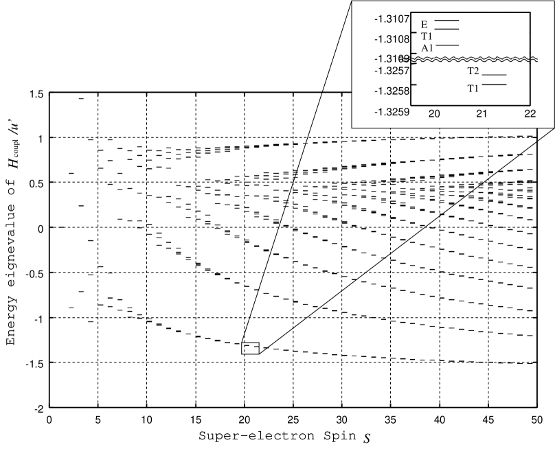
FIG. 1.: The eigenvalue of $H_{\rm coupl}/u^{\prime}$ as a function of the magnitude of Spin $S$.

FIG. 2.: The magnetic susceptibility calculated by the perturbation theory of the intermediate coupling model as a function of the ratio of coupling strength to temperature.

FIG. 3.: The profile for three coupling strength $u^{\prime}=2.24\times 10^{-4}$,$u^{\prime}=4.47\times 10^{-1}$, and $u^{\prime}=11.2$. of magnetic field $g_{\rm s}B\hbar S=0.5,2,10$. The temperature is set to $k_{\rm B}T=2$ for $g_{\rm s}B\hbar S=0.5,2$ and to $k_{\rm B}T=1$ for $g_{\rm s}B\hbar S=10$.

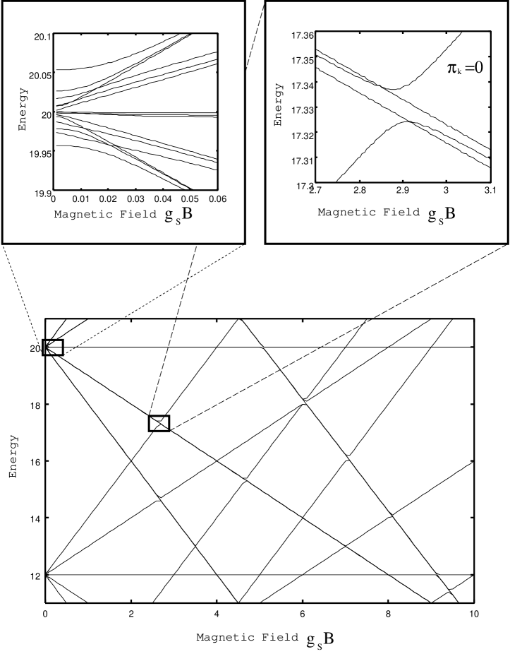
FIG. 4.: Energy levels of the weak coupling ($u^{\prime}=4.47\times 10^{-3}$) as a function of magnetic field for $S_{\rm c}=2,M=0,$ and $R\simeq 3$ or $4$.

FIG. 5.: An example of peculiar behavior of magnetization for $S_{\rm c}=2$

FIG. 6.: The second order cumulant as a function of the ratio of coupling strength and temperature. The temperature is fixed at 20.

FIG. 7.: The first order cumulant of each profile as a function of the ratio of magnetic field. The temperature is fixed at $k_{\rm B}T=1$ and for $k_{\rm B}T=2$ for Fig. 7a and Fig. 7b respectively.

FIG. 8.: The second order cumulant of each profile as a function of the ratio of magnetic field. The temperature is fixed at $k_{\rm B}T=1$ and for $k_{\rm B}T=2$ for Fig. 8a and Fig. 8b respectively.

FIG. 9.: The third order cumulant of each profile as a function of the ratio of magnetic field. The temperature is fixed at $k_{\rm B}T=1$ and for $k_{\rm B}T=2$ for Fig. 9a and Fig. 9b respectively.

REFERENCES

- [1] W.de.Heer, Paolo Milani, A.Châtelain Phys. Rev. Lett 65, 488 (1990), Isabelle M.L.Billas, Jorg A.Becker, Walt A.de Harr Z.Phys.D 26,325 (1993)
- [2] J.G.Louderback,A.J.Cox,L.J.Lising,D.C.Douglass,L.A.Bloomfield Z.Phys. D 26, 301 (1993)
- [3] D.C.Douglass, J.P.Bucher,L.A.Bloomfield, Phys. Rev. Lett. 68,1774 (1992)
- [4] A.J.Cox,J.G.Louderback,L.A.Bloomfield Phys. Rev. Lett 71, 923 (1993)
- [5] J.A.Becker, W.A.de Harr Ber.Bunsenges.Phys.Chem.96 1237 (1992)
- [6] D.C.Douglass, A.J.Cox, J.P.Bucher, L.A.Bloomfield Phys. Rev. B 47 12874 (1993)
- [7] S.N.Khanna, S.Linderoth Phys. Rev. Lett 67 742 (1991)
- [8] G.F.Bertsch, K.Yabana Phys. Rev. A 49 1930 (1994)
- [9] G.Bertsch, N.Onishi, K.Yabana Z.Phys. D 34 213 (1995)
- [10] V. Visuthikraisee and G.F. Bertsch, Phys. Rev. A54 5140 (1996)
- [11] P.Ballone, Paolo Milani, W.A.de Heer Phys. Rev. B 44 10350 (1991)
- [12] P.J.Jensen, K.H.Bennemann Z.Phys D 26 246 (1993)
- [13] A.Bohr, B.R.Mottelson Nuclear Structure vol. I