Reaction-Diffusion-Branching Models of Stock Price Fluctuations

Abstract

Several models of stock trading [P. Bak et al, Physica A 246, 430 (1997)] are analyzed in analogy with one-dimensional, two-species reaction-diffusion-branching processes. Using heuristic and scaling arguments, we show that the short-time market price variation is subdiffusive with a Hurst exponent $H=1/4$. Biased diffusion towards the market price and blind-eyed copying lead to crossovers to the empirically observed random-walk behavior ($H=1/2$) at long times. The calculated crossover forms and diffusion constants are shown to agree well with simulation data.

The movement of stock prices is among the oldest class of fluctuation phenomena that have been analyzed quantitatively [1, 2], yet very limited understanding on the origin and size of market volatilities — so fundamental to much of the finance literature[3] — is available to date. Recent empirical studies[2, 4, 5] of major financial indices around the world have revealed a number of universal features in the time series, including Levy-like distribution of short-time price moves. In search of unifying principles that explain the observed behavior, Bak, Paczuski, and Shubik (BPS)[6] recently proposed several models of stock trading among interacting agents. Their numerical study of these models suggests a rich set of dynamical behavior, including stock price fluctuations which exhibit similar statistical patterns as those of real markets[5].

From a statistical mechanical point of view, the family of models proposed by BPS are particularly interesting due to their connection to reaction-diffusion processes familiar in physical contexts[7], and thus one may hope to gain some insight into the collective behavior of traders by exploiting this analogy. A mapping between the two is easily constructed by taking the target price of agents as their coordinates on a one-dimensional price axis. The two types of agents, i.e., buyers and sellers of a stock, are identified as two species, $A$ and $B$, respectively. At any given moment, the population of buyers are separated from that of sellers by the market price $x_{M}(t)$ where transactions, or for that matter “reactions” $A+B\rightarrow\emptyset$, take place. Such reaction-diffusion problems have been studied extensively in the past[8, 9, 10, 11]. A result of particular interest is the power-law scaling of the reaction front fluctuations,

$$\langle[x_{M}(t)-x_{M}(t^{\prime})]^{2}\rangle^{1/2}\sim|t-t^{\prime}|^{H},$$ (1)

where the exponent $H=1/4$ (with possible logarithmic correction). There are, however, two new elements in the BPS models which have not been examined before: biased diffusion of $A$ and $B$ particles towards the reaction front, and price “copying” which translates to branching $A\rightarrow 2A$ and $B\rightarrow 2B$. BPS showed numerically that, in the latter case, the long time behavior of $x_{M}(t)$ changes to that of a random walk with $H=1/2$.

The purpose of this paper is to establish an analytic foundation for various observations made by BPS in their pioneering work and also to further quantify and extend their numerical results. We identify the driving force of the market price variation and determine the size of the market response from the distribution of agents near the market price. The analysis yields not only the scaling exponent $H$, but also the scaling amplitudes and various crossovers. Good agreement is reached between theoretical predictions and simulation data for a broad range of model parameters.

The original BPS model is a trading game with equal number ($N/2$) of buyers and sellers, each attaches a price $x_{i}$ to the stock they intend to buy or sell. A buyer owns no share and a seller owns exactly one share. The agents perform simultaneous, independent random walks on the price axis until they meet a member of the other group. Upon transaction, buyer and seller exchange their role and are then relocated on the price axis. In this paper we shall consider three variants of the model as detailed below:

Model I (unbiased diffusion) — The price $x_{i}$ of agent $i$ moves up or down by one unit with equal probability in each time step. For convenience, we decouple the reaction event $A+B\rightarrow\emptyset$ from the relocation of the agents in a transaction (see note [12]). A steady-state situation is maintained by injecting new agents from the two ends of a prescribed price interval at a given rate $J$.

Model II (biased diffusion) — The rules in this case are similar to those of Model I except that the updating of $x_{i}$ is biased towards the market price. Specifically, for a buyer, $x_{i}\rightarrow x_{i}+1$ with probability $(1+D)/2$ and $x_{i}\rightarrow x_{i}-1$ with probability $(1-D)/2$. The rule is reversed in the case of sellers. Obviously, Model I is regained by setting $D=0$.

Model III (biased diffusion with copying) — The updating of $x_{i}$ is the same as in Model II but now, after a transaction, the buyer and seller are immediately re-injected into the market by duplicating the price of a fellow agent chosen at random. According to BPS[6], such a process imitates herding behavior in real markets. In the particle language, it can be represented by stochastic branching $A\rightarrow 2A$ and $B\rightarrow 2B$.

We start our discussion by considering a modification of the above models which is minor from the point of view of a given diffusing particle in its whole lifetime (i.e., from its first release to the reaction), but it trivializes the problem completely. Instead of asking an $A$ particle to find a $B$ particle for a reaction, we assume that the reaction always takes place at a fixed position, say $x=0$. In essence, we are making the assumption that the market price fluctuates at a much slower rate compared to the diffusive motion of individual agents, a commonly used approximation in the study of interface fluctuations[13]. The point $x=0$ now serves as a trap of the diffusing particles which do not interact with each other. In the continuum limit, the average density of buyers $a(x,t)$ and sellers $b(x,t)$ obey the following linear equations,

$$\partial_{t}a = \gamma\partial_{x}^{2}a-\beta\partial_{x}a+S_{A},$$ (3)

$$\partial_{t}b = \gamma\partial_{x}^{2}b+\beta\partial_{x}b+S_{B},$$ (4)

with the boundary condition $a(0,t)=b(0,t)=0$. Here $\gamma$ is the diffusion coefficient of individual particles and $\beta$ describes drift towards the current market price. The updating rule of $x_{i}$ given above specifies $\beta=D$ and $\gamma=(1-D^{2})/2$ (parallel updating) or $\gamma=1/2$ (random sequential updating). The source terms $S_{A}$ and $S_{B}$ correspond to injection of new particles into the system. We now determine the steady-state solutions $a_{0}(x)$ and $b_{0}(x)=a_{0}(-x)$ to Eqs. (Reaction-Diffusion-Branching Models of Stock Price Fluctuations).

Models I and II. — The particle current

$$J=-\gamma\partial_{x}a_{0}+\beta a_{0},$$ (5)

is a constant in this case. For $\beta=0$ (Model I), the current is maintained by a linear profile [Fig. 1(a)],

$$a_{0}(x)=-Jx/\gamma.$$ (6)

For $\beta>0$ (Model II), $a_{0}(x)$ crosses over from the linear function (6) close to the origin to a constant $J/\beta$ at large distances [Fig. 1(b)],

$$a_{0}(x)=(J/\beta)[1-\exp(\beta x/\gamma)].$$ (7)

Model III. — Branching introduces source terms $S_{A}=\alpha a$ and $S_{B}=\alpha b$, where $\alpha$ is a branching rate. The equation for $a_{0}(x)$ is now a second-order ordinary differential equation which can be solved to yield,

$$a_{0}(x)=C[\exp(k_{-}x)-\exp(k_{+}x)],$$ (8)

where $k_{\pm}=(\beta\pm\sqrt{\beta^{2}-4\alpha\gamma})/(2\gamma)$ and $C$ is an overall amplitude. The steady-state solution exists only when $\alpha\leq\alpha_{c}=\beta^{2}/4\gamma$. The shape of the profile is indicated in Fig. 1(c), which is linear close to the origin and decays exponentially at large distances. The current of incoming particles at the origin is given by $J=-\gamma\partial_{x}a_{0}=\gamma C(k_{+}-k_{-})$.

FIG. 1.: Average density profiles of buyers ($a_{0}$) and sellers ($b_{0}$) along the price axis for (a) Model I (unbiased diffusion); (b) Model II (biased diffusion); (c) Model III (biased diffusion with copying). Note that in all three cases $a_{0}(x)$ and $b_{0}(x)$ vanish linearly at the market price $x_{M}$.

The total number of, say $A$ particles $n_{A}$ that arrive at the trap in a time interval $t$ to $t^{\prime}=t+\tau$ is a fluctuating quantity which can be expressed as,

$$n_{A}=\sum_{i}\eta_{i}.$$ (9)

Here the sum runs over all particles $i$ that entered the system from the beginning of the process to time $t^{\prime}$, and $\eta_{i}$ is a random variable which takes the value one if particle $i$ is trapped during the interval $\tau$ and zero otherwise. Since the $\eta_{i}$’s are independent from each other[14], we easily find,

$$\langle n_{A}\rangle = \sum_{i}p_{i},$$ (11)

$$\langle n_{A}^{2}\rangle-\langle n_{A}\rangle^{2} = \sum_{i}(p_{i}-p_{i}^{2}),$$ (12)

where $p_{i}$ is the probability that $\eta_{i}=1$. For $p_{i}\ll 1$, which holds when $\tau$ is much smaller than the typical spread of the lifetime of the diffusing particles, we have the following approximate relation,

$$\langle n_{A}^{2}\rangle-\langle n_{A}\rangle^{2}\simeq\langle n_{A}\rangle=J\tau,$$ (13)

where, as before, $J$ is the flux of particles entering the trap. Results derived below are based on this approximation but other situations may also be considered.

We now construct a heuristic argument to show how the fluctuations in $n_{A}$ and $n_{B}$ lead to a shift of the reaction front or the market price. To be definite, we take $\Delta n=n_{A}-n_{B}>0$ so that an upward move of the market price from $x_{M}$ at time $t$ to $x_{M}^{\prime}$ at time $t^{\prime}=t+\tau$ is expected (see Fig. 2). Loosely speaking, the interval $[x_{M},x_{M}^{\prime}]$ defines a reaction zone within which most of the $n_{A}$ particles entered through $x_{M}$ reacted with the $n_{B}$ particles entered through $x_{M}^{\prime}$. The excess number of $A$ particles (buyers) $\Delta n$ have either reacted with the $B$ particles initially in the zone at time $t$, or remained in the zone at the end of the period. Based on this observation, we may identify $\Delta n$ with the sum of shaded areas under $b(x,t)$ and $a(x,t^{\prime})$ in Fig. 2, respectively,

$$\Delta n \simeq \int_{x_{M}}^{x_{M}^{\prime}}a(x,t^{\prime})dx+\int_{x_{M}}^{x_{M}^{\prime}}b(x,t)dx$$ (14)

$$\simeq 2\int_{0}^{\Delta x}a_{0}(x-\Delta x)dx.$$ (15)

Here $\Delta x=x_{M}^{\prime}-x_{M}$ is the price move over the time period $\tau$. A similar relation holds for $\Delta n<0$.

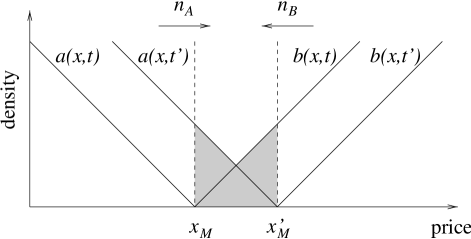
FIG. 2.: Schematic illustration of how an excess number of particles $\Delta n=n_{A}-n_{B}$ reaching the reaction zone $[x_{M},x_{M}^{\prime}]$ is accommodated by a shift of the density profiles at time $t$ to those at a later time $t^{\prime}$. Graphically, $\Delta n$ is identified with the sum of the shaded areas under $a(x,t^{\prime})$ and $b(x,t)$, respectively.

Equation (15), which holds in an average sense, is our fundamental relation that links the price move $\Delta x$ to the “demand-supply imbalance” $\Delta n$ through the density profile $a_{0}(x)$. From the statistics of $\Delta n$ we can then work out the statistics of $\Delta x$. Below we give our results on the market price fluctuations using this approach.

Model I. — In this case, the intrinsic profile $a_{0}(x)$ is linear. From Eqs. (6) and (15), we obtain $\Delta n\simeq J(\Delta x)^{2}/\gamma$. From the variance $\langle\Delta n^{2}\rangle=2J\tau$, we obtain,

$$\langle[x_{M}(t)-x_{M}(t^{\prime})]^{2}\rangle^{1/2}\simeq\bigl{(}{4\gamma^{2}\over\pi J}\bigr{)}^{1/4}|t-t^{\prime}|^{1/4}.$$ (16)

This form agrees with previous results of Refs. [9, 10, 11]. (At very short times, the discreteness of $\Delta n$ manifests itself which leads to deviations from Eq. (16). See also Ref. [8].)

Model II. — Since $a_{0}(x)$ goes to a constant for $|x|>x_{c}=\gamma/\beta$, Eq. (15) yields a linear dependence $\Delta n\simeq 2J\Delta x/\beta$ for $\Delta x>x_{c}$. Hence the move of $x_{M}(t)$ at long times is a random walk with a diffusion constant $\Gamma\simeq\langle\Delta x^{2}\rangle/2\tau=\beta^{2}/(4J)$. More detailed calculation yields a crossover scaling,

$$\langle[x_{M}(t)-x_{M}(t^{\prime})]^{2}\rangle^{1/2}\simeq x_{c}\Phi\Bigl{(}{|t-t^{\prime}|\over t_{c}}\Bigr{)},$$ (17)

where $t_{c}=\gamma^{2}J/\beta^{4}$. The limiting forms of the scaling function are given by $\Phi(s)\simeq(4s/\pi)^{1/4}$ for $s\ll 1$ and $\Phi(s)\simeq(s/2)^{1/2}$ for $s\gg 1$.

Model III. — In this case the profile (8) extends only over a finite range of $x$, so the finite lifetime of a particle becomes an important factor in our consideration. The short time behavior of the price fluctuation is similar to that of model I and II due to the linear behavior of $a_{0}(x)$ close to the origin, which is common in all three cases. Thus Eq. (16) can still be applied in this regime. Crossover to a different behavior is expected when $\tau=t^{\prime}-t$ becomes comparable to the lifetime of a particle $\tau_{0}=2\gamma/\beta^{2}$. In fact, $\tau_{0}$ is also the relaxation time of the density profiles as can be seen by bringing Eq. (Reaction-Diffusion-Branching Models of Stock Price Fluctuations) into a dimensionless form. On time intervals larger than $\tau_{0}$, memory about the initial profile is essentially lost and the next move of the market price is equally likely to be up or down, hence a random walk behavior with a step size set by the size of the fluctuation $x_{0}=\gamma^{1/2}J^{-1/4}\tau_{0}^{1/4}$ at $\tau=\tau_{0}$ [see Eq. (16)]. The usual scaling argument then yields,

$$\langle[x_{M}(t)-x_{M}(t^{\prime})]^{2}\rangle^{1/2}\simeq x_{0}\Psi\Bigl{(}{|t-t^{\prime}|\over\tau_{0}}\Bigr{)},$$ (18)

where $\Psi(s)\simeq s^{1/4}$ for $s\ll 1$ and $\Psi(s)\sim s^{1/2}$ for $s\gg 1$. The diffusion constant of the market price at long times is given by $\Gamma^{\prime}\simeq x_{0}^{2}/\tau_{0}=\beta\gamma^{1/2}J^{-1/2}$.

We have performed numerical simulations of the BPS models to check the validity of the theoretical analysis presented above. Since our results on Model I are similar to those of previous studies (apart from a possible logarithmic correction), we shall focus on Model II and III.

Model II was simulated at $J=\beta$ where the asymptotic density is one as in Ref.[6]. The system size is chosen to be $N=2000$ or larger to ensure that the reaction front does not fluctuate out of the boundaries during the time period simulated. Otherwise, $N$ is found not to have any significant effect on our results[12]. The system is first equilibrated for a period $t_{0}=10\tau_{0}$ where $\tau_{0}=N/(2\beta)$ is the typical lifetime of a particle. The market price time-series $x_{M}(t)$ is then recorded over 500 successive time segments, each of length $8192$ time steps. We then calculate $\langle[x_{M}(t)-x_{M}(t^{\prime})]^{2}\rangle$ averaged first over each time segment and then over different segments. In Fig. 3(a) we plot the simulation results using scaled variables for $D=0.01$ to 0.5. There is indeed a good data collapse over six decades. In fact, for $t>t_{c}$, not only the scaling exponent, but also the scaling amplitude are borne out by the data.

The simulation of Model III was carried out in a similar way as that of Model II, except the number of particles $N$ is now fixed. To compare the simulation data with Eq. (18), we use the relation $J=\alpha N/2$ (particle conservation) from the solution (8). Taking $\alpha=\alpha_{c}=\beta^{2}/4\gamma$[15], we obtain $x_{0}=2\gamma\beta^{-1}N^{-1/4}$. In Fig. 3(b) we plot the simulation results for market price fluctuations using the scaling suggested by Eq. (18). For four different values of $D=\beta$ and two system sizes $N=400$ and 1000, good data collapse is again achieved.

FIG. 3.: Scaling plots of the market price fluctuations versus time increments for a wide range of model parameters. (a) Model II. The value of $D$ for each data set is given in the legend. (b) Model III. The values of $D$ and $N$ for each data set are given in the legend.

In summary, we presented a heuristic method to link the market price fluctuation to the diffusive motion of individual agents using the BPS models as examples. The analysis yields qualitative as well as quantitative predictions on the size of the market price fluctuations as a function of time, the number of traders in the market, and various other model parameters. For short times, a previously known $H=1/4$ scaling law is rederived and its validity is correlated to the generic linear shape of population density profiles near the market price. Crossover to the long-time random walk behavior with $H=1/2$ takes place when agents are driven to the market price via a diffusion bias. Expressions for the crossover time as a function of various model parameters are derived. These results are shown to compare favorably with the simulation data.

The $H=1/4$ scaling at short times is quite remarkable and is against the prevailing thinking in finance that, in a market with noise traders only, there should be no restoring force to price moves and hence no correlation in the market price time series. Although the exponent is not new, the analysis presented here makes it plain that resistance to price change is inherent in the existing price distribution of agents. It remains to be elucidated how such tendencies are modified when external information (e.g., financial news) are fed into the market.

One of us (G.S.T) would like to thank the Croucher Foundation for financial support and the Physics Department, Hong Kong Baptist University for their hospitality.

REFERENCES

- [1] L. Bachelier, in The Random Character of Stock Market Prices, edited by P. H. Cootner (MIT Press, 1964), p. 17 (translation of 1900 French edition).
- [2] B. Mandelbrot, J. Business 36, 394 (1963); E. E. Peters, Fractal Market Analysis (Wiley, N.Y., 1994).
- [3] F. Black and M. Scholes, J. Political Economy 81, 637 (1973); P. Wilmott, S. Howison, and J. Dewynne, The Mathematics of Financial Derivatives (Cambridge, 1995); K. Cuthbertson, Quantitative Financial Economics (Wiley, Chichester, 1996); J. C. Hull, Options, Futures, and other Derivative Securities, 3rd Ed. (Prentice Hall, N.Y., 1997).
- [4] R. N. Mantegna and H. E. Stanley, Nature 376, 46 (1994).
- [5] For a brief review see J.-Ph. Bouchaud, to be published (http://xxx.lanl.gov/archive/cond-mat/9806101).
- [6] P. Bak, M. Paczuski, and M. Shubik, Physica A 246, 430 (1997).
- [7] A. A. Ovchinnikov, S. F. Timashev, and A. A. Belyy, Kinetics of Diffusion Controlled Chemical Processes (Nova Science, Commack, 1990).
- [8] F. Leyvraz and S. Redner, Phys. Rev. Lett. 66, 2168 (1991); E. Ben-Naim and S. Redner, J. Phys. A 25, L575 (1992).
- [9] S. Cornell and M. Droz, Phys. Rev. Lett. 70, 3824 (1993); Physica D 103, 348 (1997), and references therein.
- [10] G. T. Barkema, M. J. Howard, and J. L. Cardy, Phys. Rev. E 53, R2017 (1996).
- [11] P. Krapivsky, Phys. Rev. E 51, 4774 (1995).
- [12] Close boundary conditions impose the conservation of particle number in the system which is absent with open boundary conditions. The effect of this is to reduce the validity of Eq. (13) to much shorter times, which in turn suppresses the market price fluctuations.
- [13] S. M. Allen and J. W. Cahn, Acta. Metall. 27, 1085 (1979).
- [14] Copying in Model III introduces a weak correlation among the ’s which does not affect our argument for less than the lifetime of a particle.
- [15] In the simulations we have measured directly and observed that the ratio is slightly (up to ) bigger than one, but tends to one as increases. We however do not have a satisfactory argument on why is picked when is fixed.