Field Theoretic Approach to Long Range Reactions

Abstract

We analyze bimolecular reactions that proceed by a long-ranged reactive interaction, using a field theoretic approach that takes into account fluctuations. We consider both the one-species, $A+A\to\emptyset$ reaction and the two-species, $A+B\to\emptyset$ reaction. We consider both mobile and immobile reactants, both in the presence and in the absence of adsorption.

1 Introduction

Most chemical reactions occur through a local mechanism, where reaction occurs at a finite rate only when reactants are closer than a capture radius. In some unusual cases, however, the reaction can proceed by a long-range mechanism Forester . Exciton decay by a multipolar interaction is one such example. In these long-range cases, the rate of reaction between two reactants is distance dependent: $w(r)=\gamma/r^{n}$ for two reactants separated by a distance $r$. Here the strength of the interaction is given by $\gamma=R_{0}^{n}/\tau$, where $R_{0}$ is the Förster radius, and $\tau$ is the decay lifetime. A variety of electronic energy transfer reactions can be modeled by this form Klafter2 . More generally, an exponential form of the reaction rate may be considered, as in electron-hole recombination due to wave function overlap or barrier tunneling. The exact form of the interaction can be quite complex Klafter3 , and so even these shorter-range cases may equally well be modeled by the multipolar form, e.g. with $n=12$ Silby ; Klafter1 . A wide variety of physical systems exhibit such long-range reaction, including biological electron transport, fluorescent decay of electron-hole pairs in amorphous semiconductors, scavenging of trapped electrons in organic glasses, and decay of localized electronic states is mixed organic solids.

The case of long-range reaction has received less theoretical attention than has the more common case of local reaction. The one-species, $A+A\to\emptyset$ reaction between immobile reactants without adsorption has been investigated by placing bounds on a mean-field treatment Burlatsky2 . An interesting power-law decay of the concentration was found in $d$ spatial dimensions at long times: $c(t)\sim at^{-d/n}$ as $t\to\infty$ for $n>d$. An extension to the $A+B\to\emptyset$ case gave the scaling $c(t)\sim at^{-d/(2n-d)}$ as $t\to\infty$ for $n>d$. The single-species reaction, $A+A\to\emptyset$ reaction between immobile reactants in the presence of adsorption has been investigated with a similar treatment Oshanin2 . Adsorption corresponds to the creation of reactants, $\emptyset\to A$, with the conventional adsorption rate $J$. A non-trivial scaling of the concentration with the adsorption rate was found: $c(J)\sim aJ^{d/(n+d)}$ as $J\to 0$, $n>d$. In principle, however, these mean-field results could be modified by renormalization effects in low spatial dimensions.

In this paper, we apply the renormalization group approach to reaction kinetics to derive the asymptotically exact behavior of these long range reactions. There are eight distinct physical cases, considering all possibilities of one- or two-species reactions, with or without adsorption, and mobile or immobile reactants. Our paper is organized as follows. In section 2, we review the field theoretic approach, displaying the actions appropriate for both the one- and two-species reactions in the general case. In section 3, we derive the behavior of mobile reactants in the long-time limit in the absence of adsorption. In section 4, we derive the long-time behavior of immobile reactants in the absence of adsorption. In section 5, we derive the steady-state behavior of mobile reactants in the limit of small adsorption rates. Finally, in section 6 we derive the steady-state behavior of immobile reactants in the limit of small adsorption rates. We summarize our results in section 7.

2 Field Theoretic Formulation of Reaction Dynamics

We consider the general case of a bimolecular reaction in $d$ spatial dimensions. The reaction occurs as a result of a long-range interaction. For convenience, we define the reaction to proceed on a cubic lattice. We use a continuous-time master equation to define how the probability of any given configuration of reactants changes with time. The master equation for the $A+A\to\emptyset$ reaction is

$$\frac{\partial P(\{n_{i}\},t)}{\partial t}=$$

$$\frac{D}{h^{2}}\sum_{ij}[(n_{j}+1)P(\ldots,n_{i}-1,n_{j}+1,\ldots,t)-n_{i}P]$$

$$+\frac{1}{2}\sum_{ik}w_{ik}[(n_{i}+1)(n_{k}+1)P(\ldots,n_{i}+1,n_{k}+1,\ldots,t)$$

$$~{}~{}~{}~{}~{}~{}~{}~{}~{}~{}~{}~{}~{}~{}~{}-n_{i}n_{k}P]$$

$$+Jh^{d}\sum_{i}[P(\ldots,n_{i}-1,\ldots)-P]\ ,$$ (1)

where $h$ is the lattice spacing, $J$ is the rate of adsorption, D is the diffusivity, $n_{i}$ is the number of $A$ species on lattice site $i$, and $w_{ik}$ the distance-dependent reactive interaction. The summations over $i$ and $k$ are over all sites on the lattice, and the summation over $j$ is over all nearest neighbors of site $i$. For simplicity, we choose to place the species initially at random on the lattice, with average number density $n_{0}$.

Using the coherent state representation, we map this master equation onto a field theory Peliti ; Lee1 ; Deem1 . We find that the reactant concentration, averaged over the random initial conditions and the random statistics of the reaction-diffusion process, is

$$c_{A}(\vec{x},t)=\langle a(\vec{x},t)\rangle\ ,$$ (2)

where the average is taken with respect to $\exp(-S_{AA})$. The action is given by

$$S_{AA}=\int d^{d}\vec{x}\,\int_{0}^{t_{\rm f}}dt\,\bar{a}(\vec{x},t)\left[\partial_{t}-D\nabla^{2}+\delta(t)\right]a(\vec{x},t)$$

$$-n_{0}\int d^{d}\vec{x}\,\bar{a}(\vec{x},0)-J\int d^{d}\vec{x}\,\int_{0}^{t_{\rm f}}dt\,\bar{a}(\vec{x},t)$$

$$+\frac{1}{2}\int d^{d}\vec{x}\,d^{d}\vec{y}\,\int_{0}^{t_{\rm f}}dt\,\bar{a}(\vec{x},t)a(\vec{x},t)w(|\vec{x}-\vec{y}|)\bar{a}(\vec{y},t)a(\vec{y},t)$$

$$+\int d^{d}\vec{x}\,d^{d}\vec{y}\,\int_{0}^{t_{\rm f}}dt\,\bar{a}(\vec{x},t)a(\vec{x},t)w(|\vec{x}-\vec{y}|)a(\vec{y},t)\ .$$ (3)

The time $t_{\rm f}$ must be larger than the longest time for which we wish to make predictions. Special cases of this general formulation are given as limiting values. For immobile reactants, for example, we set $D=0$. If there is no adsorption, we set $J=0$.

For dissimilar reactants, the formulation is slightly different. The master equation is given by

$$\frac{\partial P(\{m_{i}\},\{n_{i}\},t)}{\partial t}=$$

$$\frac{D}{h^{2}}\sum_{ij}[(m_{j}+1)P(\ldots,m_{i}-1,m_{j}+1,\ldots,t)-m_{i}P]$$

$$+\frac{D}{h^{2}}\sum_{ij}[(n_{j}+1)P(\ldots,n_{i}-1,n_{j}+1,\ldots,t)-n_{i}P]$$

$$+\sum_{ik}w_{ik}[(m_{i}+1)(n_{k}+1)P(\ldots,m_{i}+1,n_{k}+1,\ldots,t)$$

$$~{}~{}~{}~{}~{}~{}~{}~{}~{}~{}~{}~{}~{}~{}~{}-m_{i}n_{k}P]$$

$$+Jh^{d}\sum_{i}[P(\ldots,m_{i}-1,\ldots)-P]$$

$$+Jh^{d}\sum_{i}[P(\ldots,n_{i}-1,\ldots)-P]\ ,$$ (4)

where now $m_{i}$ and $n_{i}$ are the number of $A$ and $B$ species, respectively, on lattice site $i$. We have assumed for simplicity that the diffusion constants of the two species are the same. So as to reach an interesting scaling regime, we have set the adsorption rates of the two species to be the same. Finally, we will set the average initial concentrations of the two reactants to be the same.

We derive the field theory from this master equation using the coherent state representation Lee2 ; Deem2 . The averaged concentrations are given by averages over two distinct fields:

$$c_{A}(\vec{x},t) = \langle a(\vec{x},t)\rangle$$

$$c_{B}(\vec{x},t) = \langle b(\vec{x},t)\rangle\ ,$$ (5)

where now the average is with respect to $\exp(-S_{AB})$. The action for dissimilar species is given by

$$S_{AB}=$$

$$\int d^{d}\vec{x}\,\int_{0}^{t_{\rm f}}dt\,\bar{a}(\vec{x},t)\left[\partial_{t}-D\nabla^{2}+\delta(t)\right]a(\vec{x},t)$$

$$+\int d^{d}\vec{x}\,\int_{0}^{t_{\rm f}}dt\,\bar{b}(\vec{x},t)\left[\partial_{t}-D\nabla^{2}+\delta(t)\right]b(\vec{x},t)$$

$$-n_{0}\int d^{d}\vec{x}\,\left[\bar{a}(\vec{x},0)+\bar{b}(\vec{x},0\right]$$

$$-J\int d^{d}\vec{x}\,\int_{0}^{t_{\rm f}}dt\,\left[\bar{a}(\vec{x},t)+\bar{b}(\vec{x},t)\right]$$

$$+\int d^{d}\vec{x}\,d^{d}\vec{y}\,\int_{0}^{t_{\rm f}}dt\,\bar{a}(\vec{x},t)a(\vec{x},t)w(|\vec{x}-\vec{y}|)\bar{b}(\vec{y},t)b(\vec{y},t)$$

$$+\int d^{d}\vec{x}\,d^{d}\vec{y}\,\int_{0}^{t_{\rm f}}dt\,\bar{a}(\vec{x},t)a(\vec{x},t)w(|\vec{x}-\vec{y}|)b(\vec{y},t)$$

$$+\int d^{d}\vec{x}\,d^{d}\vec{y}\,\int_{0}^{t_{\rm f}}dt\,\bar{b}(\vec{x},t)b(\vec{x},t)w(|\vec{x}-\vec{y}|)a(\vec{y},t)\ .$$ (6)

The long-ranged interaction shows up in the non-quadratic terms of this field theory. The vertex that we must consider for the single-species reaction is shown in figure 1.

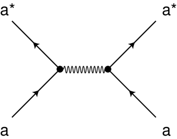
Figure 1: The vertex in the field theory of the $A+A\to 0$ reaction. Time increases in the direction of the arrows. The wavy line indicates reaction with the distance-dependent rate $w(r)$.

Similarly, the vertex we must consider in the two-species reaction is shown in figure 2.

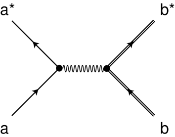
Figure 2: The vertex in the field theory of the $A+B\to 0$ reaction.

We will use both a regularized interaction

$$w_{R}(r)=\gamma/(r^{2}+R^{2})^{n/2}$$ (7)

and a pure power-law form of the interaction. The Fourier transform of the interaction is given by

$$\hat{w}_{R}(\vec{k}) = \int d^{d}\vec{r}\,\exp(i\vec{k}\cdot\vec{r})w_{R}(\vec{r})$$ (8)

$$= \frac{\gamma\pi^{d/2}(kR/2)^{(n-d)/2}}{R^{n-d}\Gamma(n/2)}2K_{(n-d)/2}(kR)\ ,$$

where $\Gamma(x)$ is the Gamma function, and $K_{l}(x)$ is the modified Bessel function of the second kind. At long-times, for low adsorption rates, the reactants tend to be widely separated, and the regularization does not affect the reaction kinetics. In the absence of regularization, we find

$$\lim_{R\to 0}[\hat{w}_{R}(0)-\hat{w}_{R}(k)] = \hat{w}(0)-\hat{w}(k)$$ (9)

$$= \frac{\gamma\pi^{d/2}\Gamma[(d-n)/2]}{2^{n-d}\Gamma(n/2)}k^{n-d}\ .$$

This equation is well-defined by the Fourier integral for $d<n<d+2$. It is derived for all other $n$ by analytic continuation from the relation $FT\{\nabla^{2}w\}=-k^{2}FT\{w\}$.

3 Mobile Reactants without Adsorption

In this section we address the simplest case of bimolecular reactions between mobile reactants in the absence of adsorption. That is, we set $J=0$ in the field-theoretic actions. We use renormalization group theory to calculate the asymptotic reactant concentrations in the long-time limit.

3.1 The $A+A\to\emptyset$ Reaction

For the single species reaction, we find the flow equations to be

$$\frac{d\ln n_{0}}{dl} = d$$

$$\frac{d\ln D}{dl} = z-2$$

$$\frac{d\ln\gamma}{dl} = z-n\ ,$$ (10)

where $z$ is the dynamical exponent. These flow equations are exact to all orders. Time renormalizes as $t(l)=e^{-zl}t$. To reach the fixed point, which requires the propagator to reach a fixed point as well, we set $z=2$. We see that the strength of the long-range reaction, $\gamma$, appears to be irrelevant when $n>2$. What this result actually implies is that the long-range nature of the reaction is irrelevant. Certainly, though, the reaction event itself is relevant. We can, therefore, use the effective interaction $w(r)=\lambda\delta(\vec{r})$. This replacement is possible only when the interaction is integrable, $n>d$, which we always require. For non-integrable interactions, the reactant concentration decays to zero immediately. The scaling for the effective reaction rate is

$$\frac{d\ln\lambda}{dl}=z-d-\frac{\lambda}{4\pi D}\ .$$ (11)

This flow equation is a one-loop expansion for small $\lambda$. The flow equations 3.1 and 11 are derived by considering the vertex corrections shown in figure 3.

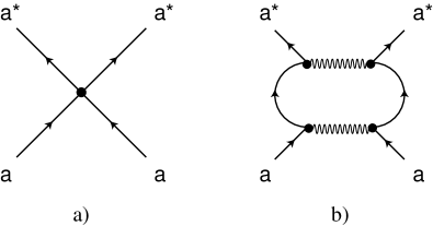
Figure 3: The local vertex and vertex correction in the field theory of the $A+A\to 0$ reaction. a) The effective local interaction, into which the non-local vertex flows. b) The vanishing correction to the non-local interaction.

The renormalization group transformation relates the original system at long times and low concentrations to another, renormalized system at short times and high concentrations. In fact, we integrate the flow equations until the renormalized time is short enough so that we can use simple mean field theory Deem1 . The matching time

$$t(l^{*})=te^{-\int_{0}^{l^{*}}z(l)dl}=t_{0}$$ (12)

is chosen to be on the order of $h^{2}/(2D)$. Calculating the renormalized reactant concentration at short times with mean field theory, we find

$$c[t(l^{*});l^{*}] = \frac{1}{1/n_{0}(l^{*})+\lambda(l^{*})t(l^{*})}$$ (13)

$$\sim \frac{1}{\lambda(l^{*})t(l^{*})}~{}\mathrm{as}~{}l^{*}\to\infty.$$

The concentration of the original system is related to that of the effective, renormalized system by scaling:

$$c(t)=e^{-dl}c[t(l);l]\ .$$ (14)

Combining equations 13 and 14, and using equation 12 to express the result in terms of $t$ rather than $l^{*}$, we find

$$c_{A}(t)\sim\left\{\begin{array}[]{ll}\frac{1}{\lambda t}&,d>2\\[7.22743pt] \frac{\ln(t/t_{0})}{8\pi Dt}&,d=2\\[7.22743pt] \frac{1}{\lambda^{*}t_{0}}\left(\frac{t}{t_{0}}\right)^{-d/2}&,d<2\end{array}\right.~{}\mathrm{as}~{}t\to\infty.$$ (15)

Here, we have used the fact that $\lambda(l)$ goes to a fixed point value for $d<2$. To first order in $2-d$, we find from equation 11 that $\lambda^{*}=4\pi D(2-d)$.

The predicted decay in equation 15 comes from assuming that the reaction will be diffusion limited at long times. This is generally true, but the results of section 4.1 show that when $d\leq 2$, the long-range nature of the reaction is relevant when $n\leq 2$. Our prediction 15, therefore, is limited to the cases of $d>2$ or $d\leq 2$ and $n>2$.

3.2 The $A+B\to\emptyset$ Reaction

For the two species reaction, we find the same flow equations as in equations 3.1 and 11. The vertex corrections that lead to this result are shown in figure 4.

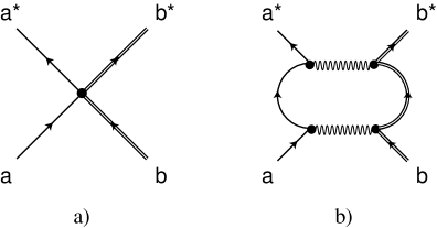
Figure 4: The vertex corrections in the field theory of the $A+B\to 0$ reaction. a) The effective local interaction, into which the non-local vertex flows. b) The vanishing correction to the non-local interaction.

As with the single species reaction, the long-range nature is irrelevant when $n>2$. At long times, the behavior of the long-range case is identical to that of the local case. This implies, as before, that $z=2$. The matching is somewhat more complicated than that of the single species reaction, due to the segregation between the $A$ and $B$ species that occurs. The result is Deem2

$$c_{A}(t)=c_{B}(t)\sim\left\{\begin{array}[]{ll}\frac{1}{\lambda t}&,d>4\\[7.22743pt] \frac{\sqrt{n}_{0}}{\sqrt{\pi}(8\pi Dt)^{d/4}}&,1\leq d<4\end{array}\right.~{}\mathrm{as}~{}t\to\infty.$$ (16)

As in section 3.1, the prediction in equation 16 is limited to the diffusion-limited regime, which section 4.2 shows occurs for $d>4$ or $d\leq 4$ and $n>4$.

In summary, for mobile reactants, the long-range nature of the reaction is irrelevant in the diffusion-limited regime. The long-time scaling of the concentration is the same as that of a reaction with a local interaction for both the one- and two-species reactions.

4 Immobile Reactants without Adsorption

The case of immobile reactants in the absence of adsorption, $D=0$ and $J=0$, is rather different. This is because for immobile reactants, the long-range and short-range cases are quite distinct. This is simply because a short-range reaction stops as soon as no more than one reactant occupies each lattice site. The long-range reaction, on the other hand, continues until either zero or one reactant remains in the entire system. As we will see, this essential difference leads to a more complicated matching procedure.

4.1 The $A+A\to\emptyset$ Reaction

As before, we use renormalization group theory to analyze the field theory in the long-time regime. Now, however, we must be careful with the definition of the interaction. We use the regularized version in equation 7. Since we are interested in the long-time regime, where the particle density is low and the particles are widely separated, we expand the interaction for large $r$:

$$w_{R}(r)=\frac{\gamma_{0}}{r^{n}}+\frac{\gamma_{2}}{r^{n+2}}+\ldots,$$ (17)

where $\gamma_{0}\equiv\gamma$. We find the flow equations to be

$$\frac{d\ln n_{0}}{dl} = d$$

$$\frac{d\ln\gamma_{i}}{dl} = z-n-i\ .$$ (18)

We immediately see that the higher order terms in the reaction rate, $\gamma_{i}$ for $i>0$, are less relevant than $\gamma_{0}$. So as to reach a fixed point, we set $z=n$. The flow equations for $n_{0}$ and $\gamma_{0}$ are then asymptotically exact.

While the regularization of the interaction $w(r)$ is irrelevant for long-times, it is important in the matching limit. Indeed, we integrate the flow equations until the density is on the order of $c[t(l^{*});l^{*}]\approx 1/R^{d}$. In that limit, we find

$$c(t_{0};l^{*})=\frac{1}{n_{0}^{-1}(l^{*})+\hat{w}(0)t_{0}}\sim\frac{1}{\hat{w}(0)t_{0}}~{}\mathrm{as}~{}l^{*}\to\infty\ ,$$ (19)

where $\hat{w}(0)=(\mathrm{const})\gamma R^{d-n}$ is not a function of $l$. We then find

$$c(t)\sim\left\{\begin{array}[]{ll}\frac{1}{\hat{w}(0)t_{0}}\left(\frac{t}{t_{0}}\right)^{-d/n}&,n>d\\[7.22743pt] 0&,n\leq d\end{array}\right.~{}\mathrm{as}~{}t\to\infty.$$ (20)

As indicated, the specific value of the cutoff affects the prefactor, but not the exponent, in the long-time scaling. When the interaction is not integrable, $n\leq d$, the concentration immediately decays to zero in the limit of a large system size.

While our treatment of this case has required use of a cutoff, the reaction process defined by the master equation is well-defined even in the absence of a cutoff. This is because any reactants experiencing the infinite reaction rate $w(0)$ simply react immediately at the onset. Indeed, in the limit $R\to 0$ and $h\to 0$, there is an exact scaling relation that relates the system at long times to a renormalized system at short times. If we rescale time as $t^{*}=\gamma n_{0}^{n/d}t$ and space as $\vec{x}^{*}=n_{0}^{1/d}\vec{x}$, we find that

$$c(\vec{x},t)=n_{0}c^{*}(\vec{x}^{*},t^{*})\ ,$$ (21)

where $c^{*}$ is the exact solution of the master equation 2 for $n_{0}=1$ and $\gamma=1$. This scaling relation explicitly demonstrates that a cutoff is not required. Indeed, this scaling relation is exactly what the renormalization group treatment is intended to derive. Essentially, this problem has so few time and length scales that the renormalization group approach does not provide any additional simplification.

On a deeper level, the scaling relation 21 implies that there is no non-trivial renormalization of the effective interaction for this problem. Mean field theory, therefore, will be accurate for both long times and short times. If we assume that there are no correlations among the reactants, we can write

$$\frac{dc}{dt}=-c\int_{R}^{\infty}dr\,S_{d}r^{d-1}\frac{\gamma}{r^{n}}c(r)\ ,$$ (22)

where $S_{d}=2\pi^{d/2}/\Gamma(d/2)$ is the surface area in $d$ dimensions. Integrating this equation using the approximation that there is only one reactant per correlated region, $c(t)\approx d/[S_{d}R^{d}(t)]$, we find

$$c(t)\sim\frac{d}{S_{d}}\left(\frac{\gamma nt}{n-d}\right)^{-d/n}~{}\mathrm{as}~{}t\to\infty,~{}~{}~{}n>d.$$ (23)

This relation gives the same power-law decay as does equation 20. Moreover, it satisfies the exact scaling relation 21. This approximate approach has essentially assumed that the radial correlation function rises from zero to unity at the average distance of interparticle separation. A more careful treatment of the correlation function would likely lead to a more accurate prefactor for the asymptotic concentration decay, without changing the exponent Kopelman .

4.2 The $A+B\to\emptyset$ Reaction

For the two-species reaction, we find the same flow equations as for the single-species reaction, equation 4.1. The matching is different, however, because the $A$ and $B$ reactants segregate in the long-time limit, just as they do in the mobile case. The segregation of the reactants requires us to adopt a different dynamical exponent. We argue that the degree of reaction between a typical reactant and a patch of reactants of volume $\Delta V$ separated by a distance $r$ is invariant at the fixed point. The typical number of reactants in a volume $\Delta V$ is proportional to $(\Delta V)^{1/2}$ in a segregated system, and so we require $\gamma(\Delta V)^{1/2}\Delta t/r^{n}$ to be invariant under the spatial and temporal rescaling in the renormalization group procedure. This condition gives $z=n-d/2$.

To analyze the matching regime, we use the mean field equations

$$\frac{\partial c_{A}}{\partial t} = -c_{A}(\vec{x},t)\int d^{d}\vec{y}\,c_{B}(\vec{y},t)w(|\vec{x}-\vec{y}|)$$

$$\frac{\partial c_{B}}{\partial t} = -c_{B}(\vec{x},t)\int d^{d}\vec{y}\,c_{A}(\vec{y},t)w(|\vec{x}-\vec{y}|)\ .$$ (24)

Since we expect segregation, we rewrite these equations in the variables $\phi=(c_{A}-c_{B})/2$ and $\rho=(c_{A}+c_{B})/2$. We make the approximation of uniform total density: $\rho(\vec{x},t)\approx\rho(t)$. This approximation is valid in the limit of weak segregation, $\phi\ll\rho$, and in the limit of strong segregation, $\rho=|\phi|$, except near domain boundaries. With this assumption, we find

$$\frac{\partial\phi}{\partial t}=\rho(\phi*w)-\phi\rho\hat{w}(0)$$ (25)

and

$$\frac{\partial\rho}{\partial t}=\phi(\phi*w)-\rho^{2}\hat{w}(0)\ .$$ (26)

Equation 25 can be solved, since $\rho$ depends on time only:

$$\hat{\phi}(\vec{k},t)=\hat{\phi}(\vec{k},0)\exp\left\{-[\hat{w}(0)-\hat{w}(k)]\int_{0}^{t}dt^{\prime}\rho(t^{\prime})\right\}\ .$$ (27)

Taking the average of equation 26 and using $\langle\phi(\vec{r},0)\phi(\vec{r}^{\prime},0)\rangle=n_{0}\delta(\vec{r}-\vec{r}^{\prime})/2$, we find

$$\frac{d\langle\rho\rangle}{dt} = \frac{n_{0}}{2}\int_{\vec{k}}\hat{w}(\vec{k})\left\langle\exp\left\{-2[\hat{w}(0)-\hat{w}(k)]\int_{0}^{t}dt^{\prime}\rho(t^{\prime})\right\}\right\rangle$$ (28)

$$-\left\langle\rho^{2}\right\rangle\hat{w}(0)\ ,$$

where the notation $\int_{\vec{k}}$ stands for $\int d^{d}\vec{k}/(2\pi)^{d}$. Note that all the terms in equation 28 scale as $e^{dl^{*}/2}$ in the matching limit. We also know that the initial reactant concentration decreases from $n_{0}e^{dl^{*}}$ to $\sqrt{n}_{0}e^{dl^{*}/2}$ in a time of the order of $1/[\hat{w}(0)n_{0}e^{dl^{*}}]$ Deem2 . Knowing this, and using the scaling relation 14, we see that the concentrations must scale as $c_{A}=c_{B}\sim(\mathrm{const})t^{-d/(2n-d)}$ in the long-time limit.

The exact scaling relation 21 also applies in this case, however, and so there are no non-mean-field effects introduced by renormalization. Knowing this, we can analyze the approximate mean-field theory 28 more thoroughly to obtain an estimate of the prefactor in the long-time decay. We perform the calculation with the non-regularized interaction of equation 9. First, we calculate the average fluctuations of $\phi$:

$$\langle\phi^{2}\rangle=\frac{n_{0}S_{d}}{2\zeta}\frac{\Gamma(d/\zeta)}{\left[2\alpha\int_{0}^{t}dt^{\prime}\rho(t^{\prime})\right]^{d/\zeta}}\ ,$$ (29)

where we have defined $\zeta=n-d$ and

$$\alpha=\frac{\gamma\pi^{d/2}\Gamma(-\zeta/2)}{2^{\zeta}\Gamma(n/2)}\ .$$ (30)

Balancing the terms in equation 26, we find that the two right-hand terms must be equal, $\rho(t)\sim|\phi(t)|$. Indeed, setting $\phi=at^{-\delta}$, we find $\delta=d/(2n-d)$. We also find an explicit form for $a$ from equation 29 by noting that since $\phi$ is a Gaussian field, $\langle|\phi(t)|\rangle=[2\langle\phi^{2}\rangle/\pi]^{1/2}$. We finally obtain

$$\langle\rho\rangle \sim n_{0}^{(n-d)/(2n-d)}\alpha^{-d/(2n-d)}\left[\frac{S_{d}\Gamma(d/\zeta)}{2\zeta}\right]^{(n-d)/(2n-d)}$$ (31)

$$\times\left(\frac{\zeta}{2n-d}\right)^{d/(2n-d)}\left(\frac{2}{\pi}\right)^{1/2}t^{-d/(2n-d)}$$

$$\mathrm{as}~{}t\to\infty,~{}~{}~{}n>d\ .$$

This exponent is in agreement with the scaling argument of Burlatsky and Chernoutsas Burlatsky2 . This result can be non-dimensionalized exactly as predicted by equation 21. Our approach here has made use of a self-consistent approximation. In particular, we integrated equation 25 by assuming that $\rho(t)$ was a given function. We then, however, made the identification $\rho=|\phi|$ to obtain the prefactor in equation 31.

As in the single-species case, we can also take a correlation function approach to the calculation of the long-time concentration profile. We have

$$\frac{dc_{A}}{dt}=-c_{A}\int_{R}^{\infty}dr\,S_{d}r^{d-1}\frac{\gamma}{r^{n}}c_{B}(r)\ .$$ (32)

Again assuming that the radial distribution function rises from zero to unity at the average interparticle separation $r=R$, we find $c_{A}(t)=\{n_{0}d/[S_{d}R^{d}(t)]\}^{1/2}$ in the segregated limit. Integrating equation 32, we find

$$c_{A}(t) = c_{B}(t)\sim n_{0}\left(\frac{2n-d}{n-d}\right)^{-d/(2n-d)}\left(\frac{d}{S_{d}}\right)^{n/(2n-d)}$$ (33)

$$\times\left(n_{0}^{n/d}\gamma t\right)^{-d/(2n-d)}~{}\mathrm{as}~{}t\to\infty,~{}~{}~{}n>d.$$

This result satisfies the exact scaling relation 21. As in the single-species case, a more accurate correlation function approach would likely lead to a better prefactor, without modification of the exponent Kopelman2 .

5 Mobile Reactants with Adsorption

We now turn to consider the case of long-range reaction of mobile reactants in the presence of adsorption. That is, we consider the general case defined by the master equations 2 or 2, with $D\neq 0$ and $J\neq 0$. To access an interesting scaling regime, we consider the limit $J\to 0$ and seek to understand how the concentration scales with $J$ in this limit.

5.1 The $A+A\to\emptyset$ Reaction

We find the flow equations for the single-species reaction to be

$$\frac{d\ln n_{0}}{dl} = d$$

$$\frac{d\ln J}{dl} = z+d$$

$$\frac{d\ln D}{dl} = z-2$$

$$\frac{d\ln\gamma}{dl} = z-n\ .$$ (34)

These flow equations are exact to all orders. We see that, as for the case of no adsorption, the long-range nature of the reaction is irrelevant when $n>2$. Of course, the presence of the reaction is important, so we set the interaction to the effective value $w(r)=\lambda\delta(\vec{r})$. We require the interaction to be integrable, $n>d$, as always. The flow equation for $\lambda$ is the same as in equation 11. To reach the fixed point, we set $z=2$. We integrate these flow equations until $J(l^{*})=e^{(2+d)l^{*}}J=J_{0}\approx D/h^{2+d}$. For this renormalized value of $J$, the average density is finite, and we can use mean field theory. The mean field theory is simple in this case, predicting

$$c[J(l^{*}),t=\infty;l^{*}]=[J(l^{*})/\lambda(l^{*})]^{1/2}\ .$$ (35)

We match the mean field result to the observed value using the scaling relation

$$c(J)=e^{-dl^{*}}c[J(l^{*});l^{*}]\ .$$ (36)

We find for the concentration in the limit $J\to 0$:

$$c(J)\sim\left\{\begin{array}[]{ll}\left(\frac{J}{\lambda}\right)^{1/2}&,d>2\\[7.22743pt] \left[\frac{J\ln(J_{0}/J)}{16\pi D}\right]^{1/2}&,d=2\\[7.22743pt] \left(\frac{J_{0}}{\lambda^{*}}\right)^{1/2}\left(\frac{J}{J_{0}}\right)^{d/(2+d)}&,d<2\end{array}\right.~{}\mathrm{as}~{}J\to 0.$$ (37)

Here, we have used the fact that $\lambda(l)$ goes to a fixed point value for $d<2$, just as it does in the case of no adsorption. These predictions are consistent with those of Rey and Droz Rey . Our argument that the long-range nature of the reaction is irrelevant is, again, valid when $d>2$ or $d\leq 2$ and $n>2$, as shown in section 6.1.

5.2 The $A+B\to\emptyset$ Reaction

For the two-species reaction, we find the same flow equations as for the single-species reaction. We also find that the local interaction dominates over the long-range component. The matching, however, is somewhat different. Again, this difference is due to the reactant segregation that can occur in low dimensions. The appropriate mean-field equations in the matching limit are

$$\frac{\partial c_{A}}{\partial t} = D\nabla^{2}c_{A}-\lambda c_{A}c_{B}+J_{A}$$

$$\frac{\partial c_{B}}{\partial t} = D\nabla^{2}c_{B}-\lambda c_{A}c_{B}+J_{B}\ ,$$ (38)

where $J_{A}$ and $J_{B}$ are random, Poisson adsorption fluxes of $A$ and $B$ reactants, respectively. Note that $\langle J_{A}\rangle=\langle J_{B}\rangle=J$. The initial conditions are irrelevant in the long time limit, since the steady state behavior is controlled by the adsorption rate. We assume for simplicity that $n_{0}=0$. These equations can be simplified and analyzed in a fashion similar to the case of no adsorption Lee2 ; Deem2 . Using the same variables as in section 4.2, we find

$$\frac{\partial\phi}{\partial t}=D\nabla^{2}\phi+\delta J$$ (39)

and

$$\frac{\partial\rho}{\partial t}=D\nabla^{2}\rho-\lambda[\rho^{2}-\phi^{2}]+\frac{J_{A}+J_{B}}{2}\ ,$$ (40)

where $\delta J=(J_{A}-J_{B})/2$. We can solve equation 39 to find

$$\hat{\phi}(\vec{k},t)=\int_{0}^{t}dt^{\prime}e^{-D(t-t^{\prime})k^{2}}\delta\hat{J}(\vec{k},t^{\prime})\ .$$ (41)

Averaging equation 40, we find

$$0=-\lambda[\langle\rho^{2}\rangle-\langle\phi^{2}\rangle]+J\ .$$ (42)

From equation 41, we find

$$\langle\phi^{2}\rangle = \lim_{t\to\infty}\int_{\vec{k}}\int_{0}^{t}dt^{\prime}e^{-2D(t-t^{\prime})k^{2}}\frac{J}{2}$$ (43)

$$= \lim_{t\to\infty}\frac{J}{2}\int_{0}^{t}dt^{\prime}\,\frac{e^{-4dDt/h^{2}}}{h^{2}}I_{0}^{d}\left(\frac{4Dt}{h^{2}}\right)$$

$$= \frac{J}{2D}f_{d}\ ,$$

where $f_{d}$ is a dimensionless numerical constant depending on the dimension. Here $I_{0}(x)$ is the modified Bessel function of the first kind. For two or fewer dimensions, $f_{d}=\infty$. We can bound the solution of equation 40 Lee2 . First, we note that since the concentrations are non-negative, $\rho\geq|\phi|$, and so $\langle\rho^{2}\rangle\geq\langle\phi^{2}\rangle$. Using this, we find

$$\langle\rho-|\phi|\rangle^{2} \leq \langle(\rho-|\phi|)^{2}\rangle$$ (44)

$$= \langle\rho^{2}\rangle+\langle\phi^{2}\rangle-2\langle\rho|\phi|\rangle$$

$$\leq \langle\rho^{2}\rangle-\langle\phi^{2}\rangle$$

$$= J/\lambda\ .$$

Combining the lower and upper bounds, we find

$$\left[\frac{Jf_{d}}{\pi D}\right]^{1/2}\leq\langle\rho\rangle\leq\left[\frac{Jf_{d}}{2D}+\frac{J}{\lambda}\right]^{1/2}\ .$$ (45)

We can immediately conclude that for a local reaction

$$\langle\rho\rangle=\infty,~{}~{}~{}d\leq 2\ .$$ (46)

This occurs because any given lattice site is dominated either by $A$ or $B$ species due to segregation. The random rate of adsorption of the dominant species is so large for $d\leq 2$ that it swamps the relaxation by diffusion of the species to nearest neighbor lattice sites, which is the only mechanism for reaction in a segregated system. Since the local reaction is ineffective for $d\leq 2$, we must reconsider our argument that the long-range component of the interaction is irrelevant. Indeed, the results of section 6.2 imply that equation 46 holds only for $n\geq 2d$.

In the matching limit, for $d>z$, the flow equations lead to

$$D(l) = De^{(z-2)l}$$

$$\lambda(l) = \lambda e^{(z-d)l}$$

$$J(l) = Je^{(z+d)l}\ ,$$ (47)

where we set $z=2$ to obtain a fixed point for the diffusivity. We define $\epsilon=J(l)f_{d}/[2D(l)]$ and note that $\epsilon\ll J(l)/\lambda(l)$. We see that

$$\langle[c_{A}(l)-c_{B}(l)]^{2}\rangle=4\epsilon$$ (48)

and

$$\langle[c_{A}(l)+c_{B}(l)]^{2}\rangle=\frac{4J(l)}{\lambda(l)}+4\epsilon\ .$$ (49)

We note that equation 43 implies, since $\phi$ is a Gaussian field,

$$\langle|c_{A}(l)-c_{B}(l)|\rangle=2\left[\frac{2\epsilon}{\pi}\right]^{1/2}\ .$$ (50)

This implies that $c_{A}(l)$ and $c_{B}(l)$ fluctuate in the same way: $c_{A}(l)\sim c_{B}(l)+O(\sqrt{\epsilon})$. Since $\langle\rho^{2}(l)\rangle=\langle\phi^{2}(l)\rangle+J(l)/\lambda(l)$, we find $\langle c_{A}(l)^{2}\rangle=\langle c_{B}(l)^{2}\rangle=J(l)/\lambda(l)+O(\epsilon)$. Using $\langle c_{i}(l)^{2}\rangle=\langle c_{i}(l)\rangle^{2}+\langle[\delta c_{i}(l)]^{2}\rangle$ and equations 48 and 49, we find $\langle[\delta c_{A}(l)]^{2}\rangle=\langle[\delta c_{B}(l)]^{2}\rangle=O(\epsilon)$. Since the fluctuations are much smaller than the mean, we can finally conclude that

$$\langle c_{A}(l)\rangle=\langle c_{B}(l)\rangle\sim\left[\frac{J(l)}{\lambda(l)}\right]^{1/2}~{}\mathrm{as}~{}J\to 0,~{}~{}~{}d>2\ .$$ (51)

Since the scaling predicted by the flow equations is trivial, this result holds for the observable concentrations as well:

$$\langle c_{A}\rangle=\langle c_{B}\rangle\sim\left\{\begin{array}[]{ll}\left(\frac{J}{\lambda}\right)^{1/2}&,d>2\\[7.22743pt] \infty&,d\leq 2\end{array}\right.~{}\mathrm{as}~{}J\to 0.$$ (52)

6 Immobile Reactants with Adsorption

We now consider the final case of immobile reactants in the presence of adsorption. We consider the regime $J\to 0$, which leads to non-trivial scaling of the reactant concentration with the adsorption rate. As in section 4, we will find that the decay rate depends sensitively on the interaction $w(r)$.

6.1 The $A+A\to\emptyset$ Reaction

For the single species reaction, we find the same flow equations and dynamical exponent as in section 4.1, with the additional equation for the adsorption rate

$$\frac{d\ln J}{dl}=z+d\ .$$ (53)

As in section 4.1, we find that while simple scaling arguments predict the local reaction mechanism to dominate over the long-range reaction mechanism, this is actually not the case. In the low-concentration, small-$J$ limit, the reaction proceeds only by the long-range mechanism for immobile reactants. In the matching limit, we find $c[J(l^{*});l^{*}]=[J(l^{*})/J_{0}]^{1/2}$, where $J_{0}\approx\gamma h^{-d-n}$. The observable concentration is given by the scaling relation $c(J)=e^{-dl^{*}}c[J(l^{*});l^{*}]$, where $l^{*}$ is chosen so that $J(l^{*})=J_{0}$. Performing the matching, we find

$$c(J)\sim\left\{\begin{array}[]{ll}\left(\frac{J}{J_{0}}\right)^{d/(n+d)}&,n>d\\[7.22743pt] \infty&,n\leq d\end{array}\right.~{}\mathrm{as}~{}J\to 0.$$ (54)

This result is the same as that found by Oshanin and coworkers using an approximate, mean-field approach Oshanin2 .

We can also find an exact scaling relation for this problem. Defining $\vec{x}^{*}=(J/\gamma)^{1/(n+d)}\vec{x}$ and $t^{*}=J(\gamma/J)^{d/(n+d)}t$, we find

$$c(\vec{x},t)=\left(\frac{J}{\gamma}\right)^{d/(n+d)}c^{*}(\vec{x}^{*},t^{*})\ ,$$ (55)

where $c^{*}$ satisfies the exact master equation 2 with $J=1$ and $\gamma=1$. This scaling relation implies that $\langle c\rangle=(\mathrm{const})(J/\gamma)^{d/(n+d)}=(\mathrm{const})(J/J_{0})^{d/(n+d)}$, which is exactly what we found in equation 54.

6.2 The $A+B\to\emptyset$ Reaction

For the two-species reaction, we find the same flow equations and dynamical exponent as in section 4.2, with the addition of equation 53. In the matching limit, we can use a similar type of mean field theory:

$$\frac{\partial\phi}{\partial t}=\rho(\phi*w)-\phi\rho\hat{w}(0)+\delta J$$ (56)

and

$$\frac{\partial\rho}{\partial t}=\phi(\phi*w)-\rho^{2}\hat{w}(0)+(J_{A}+J_{B})/2\ .$$ (57)

Equation 56 can be solved, since $\rho$ depends on time only:

$$\hat{\phi}(\vec{k},t) = \int_{0}^{t}dt^{\prime}\exp\left\{-\int_{t^{\prime}}^{t}dt^{\prime\prime}[\hat{w}(0)-\hat{w}(k)]\rho(t^{\prime\prime})\right\}$$ (58)

$$\times\delta\hat{J}(\vec{k},t^{\prime})\ .$$

Taking the average of equation 57 and using equation 58 and $\langle\delta\hat{J}(\vec{k},t^{\prime})\delta\hat{J}(\vec{k}^{\prime},t^{\prime\prime})\rangle=(J/2)\delta(t^{\prime}-t^{\prime\prime})(2\pi)^{d}\delta(\vec{k}-\vec{k}^{\prime})$, we find

$$\frac{d\langle\rho\rangle}{dt} = \frac{J}{2}\int_{0}^{t}dt^{\prime}\int_{\vec{k}}$$ (59)

$$\times\hat{w}(\vec{k})\left\langle\exp\left\{-2\int_{t^{\prime}}^{t}dt^{\prime\prime}[\hat{w}(0)-\hat{w}(k)]\rho(t^{\prime\prime})\right\}\right\rangle$$

$$-\left\langle\rho^{2}\right\rangle\hat{w}(0)+J\ .$$

In the long-time limit, the average density goes to a constant. In this limit, then,

$$0=\frac{J}{2}\int_{\vec{k}}\frac{\hat{w}(\vec{k})}{2[\hat{w}(0)-\hat{w}(\vec{k})]\rho}-\rho^{2}\hat{w}(0)+J\ .$$ (60)

Using the explicit expression 9 for the interaction, we can evaluate the first integral:

$$\int_{\vec{k}}\frac{\hat{w}(\vec{k})}{\hat{w}(0)-\hat{w}(k)} = (\mathrm{const})\int_{0}^{\Lambda}dk\,\hat{w}(k)k^{d-\zeta-1}\ ,$$ (61)

$$< \infty,~{}~{}~{}~{}~{}~{}d>\zeta\ .$$

Here $\Lambda=2\pi/h$ is the cutoff in Fourier space, and we have concentrated on the small-$k$, large-distance properties of this integral. Since $\zeta=n-d$, we see that the integral converges to a finite value only for $n<2d$. When the integral converges, the first term in equation 60 is subdominant, because $\rho$ is large in the matching limit, and by performing the matching we find the expected mean-field behavior. In the case of $n\geq 2d$, the average density diverges, as we can see explicitly from the bound $\langle\rho\rangle\geq\langle|\phi|\rangle$, since $\langle\phi^{2}\rangle=(\mathrm{const})\int_{0}^{\Lambda}dk\,k^{d-\zeta-1}$ diverges for $n\geq 2d$. The final result is

$$c_{A}=c_{B}\sim\left\{\begin{array}[]{ll}\infty&,n\geq 2d\\[7.22743pt] \left(\frac{J}{J_{0}}\right)^{d/(n+d)}&,d<n<2d\\[7.22743pt] 0&,n\leq d\end{array}\right.~{}\mathrm{as}~{}J\to\ 0.$$ (62)

This result satisfies the exact scaling relation 55, as it must.

Interestingly, if the interaction decays too quickly with distance, $n\geq 2d$, then segregation occurs, and the adsorption swamps the reaction rate. This effect can only occur in the $A+B\to 0$ case, where the density of a majority species can grow without bound on a lattice site. If the interaction is sufficiently long-ranged, $d<n<2d$, then segregation is prevented, and the reaction proceeds as in the homogeneous, single-species case. As always, if the interaction is not integrable, $n\leq d$, the concentration is forced to vanish in the limit of a large system.

7 Summary

Using a field-theoretic formulation of reaction kinetics, we have derived the asymptotic behavior of long-ranged, bimolecular reactions. When the reactants are mobile, the long-ranged nature of the reaction is usually irrelevant. Conversely, when the reactants are immobile, the long-ranged reactive interaction is crucial for the reaction to proceed. In the $A+A\to\emptyset$ reaction, concentration fluctuations are only mildly important. The reactants in the $A+B\to\emptyset$ reaction, however, typically segregate in the absence of adsorption. Adsorption tends either to homogenize or to drive the system to infinite density in the $A+B\to\emptyset$ reaction.

References

• (1) T. FΓΆrster, Z. Naturforschg. A 4, 321 (1949).
• (2) J. Klafter and J. Jortner, J. Chem. Phys. 73, 1004 (1980).
• (3) J. Klafter, A. Blumen, and J.Β M. Drake, in Molecular Dynamics is Restricted Geometries, edited by J. Klafter and J.Β M. Drake (Wiley, New York, 1989), p.Β 1.
• (4) A. Blumen and R. Silbey, J. Chem. Phys. 70, 3707 (1979).
• (5) J. Klafter, A. Blumen, and G. Zumofen, J. Phys. Chem. 87, 191 (1983).
• (6) S.Β F. Burlatsky and A.Β I. Chernoutsas, Phys. Lett. A 145, 56 (1990).
• (7) G. Oshanin etΒ al., J. Phys. Chem. 98, 7390 (1994).
• (8) L. Peliti, J. Phys. A 19, L365 (1986).
• (9) B.Β P. Lee, J. Phys. A 27, 2633 (1994).
• (10) J.-M. Park and M.Β W. Deem, Phys. Rev. E 57, 3618 (1998).
• (11) B.Β P. Lee and J. Cardy, J. Stat. Phys. 80, 971 (1995); 87, 951 (1997).
• (12) M.Β W. Deem and J.-M. Park, Phys. Rev. E 57, 2681 (1998).
• (13) K. Lindenberg, P. Argyrakis, and R. Kopelman, J. Phys. Chem. 99, 7542 (1995).
• (14) K. Lindenberg, B.Β J. West, and R. Kopelman, Phys. Rev. A 42, 890 (1990).
• (15) P.Β A. Rey and M. Droz, J. Phys. A 30, 1101 (1997); equation 28 contains sign errors in the exponent and argument of the $\ln J$ term.