Abstract

A homogeneous Bose gas is investigated at finite temperature using renormalization group techniques. A non–perturbative flow equation for the effective potential is derived using sharp and smooth cutoff functions. Numerical solutions of these equations show that the system undergoes a second order phase transition in accordance with universality arguments. We obtain the critical exponent $\nu=0.73$ to leading order in the derivative expansion.

I Introduction

The remarkable achievement of Bose–Einstein condensation (BEC) of alkali atoms in magnetic traps [1–3] has created an enormous interest in the properties of dilute Bose gases. A very recent review on the trapped Bose gases can be found in Ref. [4] and an overview in Ref. [5]. However, it is useful to gain insight into the simpler problem of an interacting homogeneous Bose gas by applying modern methods from thermal field theory before attacking the full problem of atoms trapped in an external potential.

The homogeneous Bose gas at zero temperature was intensively studied in the 1950s [6, 7]. The properties of this system can be calculated in an expansion of powers of $\sqrt{\rho a^{3}}$, where $\rho$ is the density of the gas and $a$ is the S–wave scattering length. At zero temperature this expansion is equivalent to the loop expansion. The leading quantum correction to the ground state energy was calculated in 1957 by Lee and Yang [6]. The complete two–loop result was recently obtained by Braaten and Nieto [8].

The system has also been investigated at finite temperature. Since this model is in the same universality class as the three–dimensional $xy$–model, one expects the phase transition to be second order [9]. However, both Bogoliubov theory [6] and two–body $t$–matrix theory [10] predict a first order phase transition. They fail because they do not take into account many–body effects of the medium [11]. In order to resolve this problem, Bijlsma and Stoof used a many–body $t$–matrix approximation [11]. In this approximation the propagators are self–consistently determined in the self-energy diagrams (in contrast with the Bogoliubov theory, where free propagators are used in the self-energy graphs). This approach yields a second order phase transition, but predicts the same critical temperature as that of a non–interacting gas.

Haugset, Haugerud and Ravndal [12] have recently studied the phase transition of this system. By self–consistently solving a gap equation for the effective chemical potential, they are effectively summing up daisy and superdaisy diagrams. The inclusion of these diagrams is essential in order to satisfy the Goldstone theorem at finite temperature. Within this approximation the phase transition is second order, but there is no correction to $T_{c}$ compared with the non–interacting gas.

One very powerful method of quantum field theory is the Wilson renormalization group (RG) [13, 14]. Renormalization group techniques have been applied to a homogeneous Bose gas by several authors [15–18]. Bijlsma and Stoof have made an extensive quantitative study of this system and in particular calculated non–universal quantities such as the critical temperature and the superfluid fraction below $T_{c}$ [19]. The non–universal quantities depend on the details of the interactions between the atoms. Using renormalization group methods, they demonstrate that the phase transition is indeed second order, and that the critical temperature increases by approximately 10% for typical alkali atoms compared with that of a free Bose gas. A review summarizing the current understanding of homogenous Bose gases can be found in [20].

The critical exponents for the phase transition from a superfluid to a normal fluid observed in liquid ⁴He have been measured very accurately [9]. On the theoretical side, the most precise calculations to date involve the $\epsilon$–expansion. The agreement between the five loop calculations up to $\epsilon^{5}$ and experiment is excellent, but one should bear in mind that the series is actually asymptotic. The $\epsilon$–expansion works extremely well for scalar theories, but not for gauge theories [21], and so it is important to have alternative methods to compute the critical exponents. The momentum shell renormalization group provides one such alternative, and the literature on the calculational techniques for obtaining the critical exponents is now vast [22–26].

In the present work we reconsider the nonrelativistic homogeneous spin zero–Bose gas at finite temperature using RG techniques including higher order operators than was done in Ref [19]. We focus in particular on the critical behavior and the calculation of critical exponents. The paper is organized as follows. In section II we briefly discuss the symmetries and interactions underlying the effective Lagrangian of the Bose gas. In section III the renormalization group is discussed, and we derive the flow equation for the one–loop effective potential. In section IV the flow equation for the one-loop RG–improved effective potential is found. In section V we calculate fixed points and critical exponents, using different cutoff functions and we address the question of scheme dependence of the results for the critical exponents [25]. In section VI we summarize and conclude. In the Appendix we prove that the one–loop renormalization group flow equation is exact to leading order in the derivative expansion. Throughout the paper we use the imaginary time formalism.

II Effective Lagrangian

In this section we briefly summarize the symmetries and interactions underlying the effective Lagrangian of a dilute Bose gas. A more detailed description can be found in [5, 27].

The starting point of the description of a homogeneous Bose gas is an effective quantum field theory valid for low momenta [28]. As long as the momenta $p$ of the atoms are small compared to their inverse size, the interactions are effectively local and we can describe them by a local quantum field theory. Since the momenta are assumed to be so small that the atoms are nonrelativistic, the Lagrangian is invariant under Galilean transformations. There is also an $O(2)$–symmetry, and for simplicity we take the atoms to have either have zero spin or to be maximally polarized. We can then describe them by a single complex field:

$$\psi={1\over\sqrt{2}}\left[\psi_{1}+i\psi_{2}\right].$$ (1)

The interactions of two atoms can be described in terms of a two-body potential $V({\bf r}_{1}-{\bf r}_{2})$. The potential is repulsive at very short distances and there is an attractive well. Finally, there is a long–range Van der Waals tail that behaves like $1/R^{6}$. For the example of ⁸⁷Rb the minimum of the well is around $R_{0}=5a_{0}$, where $a_{0}$ is the Bohr radius. The depth is approximately $0.5$ eV and there are around 100 molecular bound states in the well. The S-wave scattering lengths $a$ of typical alkali atoms are much larger than $R_{0}$ (e.g. $a\approx 110a_{0}$ for ⁸⁷Rb) because the natural scale for the scattering length is set by the Van der Waals interaction [5].

The Euclidean effective Lagrangian then reads

$${\cal L}_{E}=\psi^{\dagger}\partial_{\tau}\psi+\nabla\psi^{\dagger}\cdot\nabla\psi-\mu\psi^{\dagger}\psi+g(\psi^{\dagger}\psi)^{2}+\ldots\,.$$ (2)

Here, $\mu$ is the chemical potential. We have set $\hbar=1$ and $2m=1$. The interaction $g(\psi^{\dagger}\psi)^{2}$ represents $2\rightarrow 2$ scattering and the coupling constant $g$ is proportional to the $S$–wave scattering length $a$:

$$g=4\pi a.$$ (3)

The ellipses indicate all symmetry preserving operators that are higher order in the number of fields and derivatives.

In the following we consider the dilute gas $\rho a^{3}\ll 1$, which implies that we only need to retain the quartic interaction in the bare Lagrangian Eq. (2) [19].

The action can be written as

$$S\left[\psi_{1},\psi_{2}\right]=\int_{0}^{\beta}d\tau\int d^{d}x\Bigg{\{}{i\over 2}\epsilon_{ij}\psi_{i}\partial_{\tau}\psi_{j}+{1\over 2}\nabla\psi_{i}\cdot\nabla\psi_{i}+{g\over 4}(\psi_{i}\psi_{i})^{2}\Bigg{\}},$$ (4)

where $d$ is the number of spatial dimensions and repeated indices are summed over.

In a field theoretic language, BEC is described as spontaneous symmetry breaking of the $O(2)$–symmetry and the complex field $\psi$ acquires a nonzero vacuum expectation value $v$. Due to the $O(2)$–symmetry, the field $v$ can be chosen to be real and so we shift the fields according to

$$\psi_{1}\rightarrow v+\psi_{1},\hskip 19.91684pt\psi_{2}\rightarrow\psi_{2}.$$ (5)

Inserting (5) into (4) and dividing the action into a free piece $S_{\mbox{free}}[\psi_{1},\psi_{2}]$ and an interacting part $S_{\mbox{int}}[\psi_{1},\psi_{2}]$ we obtain

$$S_{\mbox{free}}[v,\psi_{1},\psi_{2}] = \int_{0}^{\beta}d\tau\int d^{d}x\left\{-{1\over 2}\mu v^{2}+{i\over 2}\psi_{i}\epsilon_{ij}\partial_{\tau}\psi_{j}+\frac{1}{2}\psi_{1}\left[-\nabla^{2}+V^{\prime}+V^{\prime\prime}v^{2}\right]\psi_{1}\right.$$ (7)

$$+\left.\frac{1}{2}\psi_{2}\left[-\nabla^{2}+V^{\prime}\right]\psi_{2}\right\}$$

$$S_{\mbox{int}}[v,\psi_{1},\psi_{2}] = \int_{0}^{\beta}d\tau\int d^{d}x\Bigg{\{}{g\over 4}\left[v^{4}+4v\psi_{1}^{3}+4v\psi_{2}^{3}+\psi_{1}^{4}+2\psi_{1}^{2}\psi_{2}^{2}+\psi^{4}_{2}\right]\Bigg{\}}.$$ (8)

Here $V(v)$ is the classical potential

$$V(v)=-{1\over 2}\mu v^{2}+{g\over 4}v^{4}.$$ (9)

We will use primes to denote differentiation with respect to $v^{2}/2$, so that $V^{\prime}=-\mu+gv^{2}$ and $V^{\prime\prime}=2gv^{2}$.

The free propagator corresponding to Eq. (7) is a $2\times 2$ matrix and in momentum space it reads

$$\Delta(\omega_{n},p)=\frac{1}{\omega_{{p}}^{2}+\omega_{n}^{2}}\left(\begin{array}[]{cc}\epsilon_{p}+V^{\prime}&\omega_{n}\\ -\omega_{n}&\epsilon_{p}+V^{\prime}+V^{\prime\prime}v^{2}\end{array}\right),$$ (12)

where

$$\epsilon_{p} = p^{2}$$ (13)

$$\omega_{n} = 2\pi nT$$ (14)

$$\omega_{p} = \sqrt{\left[\epsilon_{p}+V^{\prime}+V^{\prime\prime}v^{2}\right]\left[\epsilon_{p}+V^{\prime}\right]}.$$ (15)

In the broken phase the quadratic part of the action, Eq. (7), describes the propagation of Bogoliubov modes with the dispersion relation

$$\omega_{p}=p\sqrt{\epsilon_{p}+2\mu}.$$ (16)

The dispersion is linear in the long wavelength limit, corresponding to the massless Goldstone mode (phonons). This reflects the spontaneous symmetry breakdown of the $O(2)$ symmetry. In the short wavelength limit the dispersion relation is quadratic and that of a free nonrelativistic particle.

III The One–Loop Effective Potential at Finite Temperature

We are now ready to calculate quantum corrections to the classical potential Eq. (15). In this section we compute the one–loop effective potential which we will “RG improve” in the next section. This method of deriving RG flow equations is conceptually and technically simpler than the direct application of exact or momentum-shell RG techniques which is demonstrated in the Appendix.

The one-loop effective potential reads

$$U_{\beta}(v) = V(v)+\mbox{Tr}\ln\Delta^{-1}(\omega_{n},p)$$ (17)

$$= -{1\over 2}\mu v^{2}+{g\over 4}v^{4}+{1\over 2}T\sum_{n}\int{d^{d}p\over(2\pi)^{d}}\ln[\omega_{n}^{2}+\omega_{p}^{2}].$$ (18)

The sum is over the Matsubara frequencies, which take on the values $\omega_{n}=2\pi nT$, and the integration is over $d$–dimensional momentum space.

We proceed by dividing the modes in the path integral into slow and fast modes separated by an infrared cutoff $k$. This is done by introducing a cutoff function $R_{k}(p)$ which we keep general for the moment. By adding a term to the action Eq. (4):

$$S_{\beta,k}[\psi_{1},\psi_{2}]=S[\psi_{1},\psi_{2}]+\int_{0}^{\beta}d\tau\int d^{3}x\,\mbox{$1\over 2$}R_{k}(\sqrt{-\nabla^{2}})\nabla\psi_{i}\cdot\nabla\psi_{i},$$ (19)

the modified propagator reads

$$\Delta_{k}(\omega_{n},p)=\frac{1}{\omega_{{p}}^{2}+\omega_{n}^{2}}\left(\begin{array}[]{cc}\epsilon_{p}(R_{k}(p)+1)+V^{\prime}&\omega_{n}\\ -\omega_{n}&\epsilon_{p}(R_{k}(p)+1)+V^{\prime}+V^{\prime\prime}v^{2}\end{array}\right),$$ (22)

and the modified dispersion relation is

$$\omega_{p,k} = \sqrt{\left[\epsilon_{p}(R_{k}(p)+1)+V^{\prime}+V^{\prime\prime}v^{2}\right]\left[\epsilon_{p}(R_{k}(p)+1)+V^{\prime}\right]}.$$ (23)

By a judicious choice of $R_{k}(p)$, we can suppress the low momentum modes in the path integral and leave the high momentum modes essentially unchanged. In section V we return to the actual choice of cutoff functions. It is useful to introduce a blocking function $f_{k}(p)$ which is defined through

$$R_{k}(p)={1-f_{k}(p)\over f_{k}(p)}.$$ (24)

The blocking function satisfies

$$\lim_{p\rightarrow 0}f_{k}(p)=0,\hskip 28.45274pt\lim_{p\rightarrow\infty}f_{k}(p)=1.$$ (25)

This implies that the function $R_{k}(p)$ satisfies

$$\lim_{p\rightarrow 0}R_{k}(p)=\infty,\hskip 28.45274pt\lim_{p\rightarrow\infty}R_{k}(p)=0.$$ (26)

These properties ensure that the low–momentum modes are suppressed by making them very heavy and the high–momentum modes are left essentially unchanged.

We return to the one–loop effective potential, which now becomes

$$U_{\beta,k}(v)=V(v)+{1\over 2}T\sum_{n}\int{d^{d}p\over(2\pi)^{d}}\ln\left[\omega_{n}^{2}+\omega_{p,k}^{2}\right].$$ (27)

Here, the subscript $k$ indicates that the effective potential depends on the infrared cutoff. Upon summation over the Matsubara frequencies, we obtain

$$U_{\beta,k}(v)=V(v)+\frac{1}{2}\int{d^{d}p\over(2\pi)^{d}}\bigg{[}\omega_{{p,k}}+2T\ln\left[1-e^{-\beta\omega_{{p,k}}}\right]\bigg{]}.$$ (28)

The first term in the brackets is the $T=0$ piece and represents the zero–point fluctuations. The second term includes thermal effects. Differentiation with respect to the infrared cutoff $k$ yields:

$$k{\partial\over\partial k}U_{\beta,k}=-{k\over 2}\int{d^{d}p\over(2\pi)^{d}}\left({\partial R_{k}\over\partial k}\right)\left[{1\over 2\omega_{p,k}}+{1\over\omega_{p,k}(e^{\beta\omega_{p,k}}-1)}\right]\left[2\epsilon_{p,k}+2V^{\prime}+V^{\prime\prime}v^{2}\right].$$ (29)

Eq. (29) is the differential equation for the one–loop effective potential. It is obtained by integrating out each mode independently, where the feedback from the fast modes to the slow modes is completely ignored. Since all modes are integrated out independently, this is sometimes called the independent mode approximation [29].

Equation (28) provides an inadequate description of the system at finite temperature in several ways. Since the minimum of the one-loop effective potential at finite temperature is shifted away from the classical minimum, the Goldstone theorem is not satisfied. This theorem is known to be satisfied for temperatures below $T_{c}$ to all orders in perturbation theory [30], and any reasonable approximation must incorporate that fact.

Secondly, it is clear from Eqs. (23) and (28) that the one-loop effective potential has an imaginary part for all temperatures and for sufficiently small values of the field $v$, when the bare chemical potential is positive. However, we know that a thermodynamically stable state for $T\geq T_{c}$ corresponds to $v=0$ and so the effective potential is purely real for sufficiently high temperatures. More generally, ordinary perturbation theory breaks down at high temperature due to infrared divergences and this has been known since the work on summation of ring diagrams in nonrelativistic QED in 1957 by Gell-Mann and Brückner [31]. In the next section we derive an RG equation, whose solution has none of the above shortcomings.

IV Renormalization Group Improvement

In the previous section we derived the one–loop effective potential at finite temperature and discussed the fact that it is not capable of reliably describing the system at finite temperature. The lack of feedback from the fast modes to the slow modes as we lower the infrared cutoff $k$ leads to a poor tracking of the effective degrees of freedom causing the problems mentioned above. The situation is remedied by applying the renormalization group, which effectively sums up important classes of Feynman diagrams [26]. In order to obtain the differential equation for the RG–improved effective potential, we do not integrate out all the modes between $p=\infty$ and $p=k$ in one step. Instead, we divide the integration volume into small shells of thickness $\Delta k$, then lower the cutoff from $k$ to $k-\Delta k$ and repeat the one-loop calculation. This is equivalent to replacing $V$ by $U_{\beta,k}$ on the right hand side of Eq. (29), making it self–consistent [29]:

$$k{\partial\over\partial k}U_{\beta,k}=-{k\over 2}\int{d^{d}p\over(2\pi)^{d}}\left({\partial R_{k}\over\partial k}\right)\left[{1\over 2\omega_{p,k}}+{1\over\omega_{p,k}(e^{\beta\omega_{p,k}}-1)}\right]\left[2\epsilon_{p}+2U_{\beta,k}^{\prime}+U_{\beta,k}^{\prime\prime}v^{2}\right],$$ (30)

where

$$\omega_{p,k}=\sqrt{\left[\epsilon_{p}(R_{k}(p)+1)+U^{\prime}_{\beta,k}+U^{\prime\prime}_{\beta,k}v^{2}\right]\left[\epsilon_{p}(R_{k}(p)+1)+U^{\prime}_{\beta,k}\right]},$$ (31)

and the primes in Eqs. (30) and (31) denote differentiation with respect to $v^{2}/2$. The self–consistent Eq. (30) is not a perturbative approximation, but is exact to leading order in the derivative expansion. This equation is derived in the Appendix without performing a loop expansion.

Note that since

$$2v{\partial U_{\beta,k}\over\partial v^{2}}={\partial U_{\beta,k}\over\partial v},$$ (32)

the dispersion relation at the minimum of the effective potential in the broken phase reduces to

$$\omega_{p,k=0}=p\sqrt{\epsilon_{p}+U^{\prime\prime}_{\beta,k=0}v^{2}}.$$ (33)

Hence, the Goldstone theorem is automatically satisfied for temperatures below $T_{c}$.

This equation interpolates between the bare theory for $k=\infty$ and $T=0$ and the physical theory at temperature $T$, for $k=0$, since we integrate out both quantum and thermal modes as we lower the cutoff. This implies that the boundary condition for the RG–equation is the bare potential, $U_{\beta,k=\infty}(v)=V(v)$.

In Refs. [32, 33] renormalization group ideas have been applied to $\lambda\phi^{4}$ theory using the real time formalism. In the real time formalism one can separate the free propagator into a quantum and a thermal part [34], and in [32, 33] the infrared cutoff is imposed only on the thermal part of the propagator. This implies that the theory interpolates between the physical theory at $T=0$ and the physical theory at $T\neq 0$. Hence, the boundary condition for the RG–equation in this approach is the physical effective potential at $T=0$. However, if one imposes the infrared cutoff on the both quantum and thermal part of the propagator, one can derive Eq. (30), showing that identical results are obtained using the two formalisms.

We close this section by commenting on the choice of cutoff function. It is clear from Eq. (30) that the non-perturbative flow equation depends explicitly on the choice of $R_{k}(p)$. We know that the nonzero Matsubara modes are strongly suppressed at high temperature and can be integrated out perturbatively; the important point is to treat the zero mode correctly. For a thorough discussion of various finite temperature cutoff functions applied to relativistic $\lambda\phi^{4}$ theory see Ref. [35].

V Results

In this section we present our results for the numerical solution of the renormalization group flow equation and the calculations of the fixed point and critical exponents. We consider the cases of a sharp cutoff and a smooth cutoff separately.

A Sharp Cutoff

The sharp cutoff function is defined by the blocking function $f_{k}(p)=\theta(p-k)$, which is displayed in Fig 6 (solid line). It provides a sharp separation between fast and slow modes. Using the sharp cutoff the slow modes become completely suppressed in the path integral, while the fast modes are completely unaltered. The advantage of using the sharp cutoff function compared to the smooth cutoff functions considered in section V B is that the integral over $p$ can be done analytically, resulting in a differential RG–equation. In this case Eq. (30) reduces to

$$k\frac{\partial}{\partial k}U_{\beta,k}=-{1\over 2}S_{d}k^{d}\Bigg{[}\omega_{k}+2T\ln\left[1-e^{-\beta\omega_{{k}}}\right]\Bigg{]}.$$ (34)

Here,

$$\omega_{{k}} = \sqrt{\left[\epsilon_{k}+U^{\prime}_{\beta,k}+U^{\prime\prime}_{\beta,k}v^{2}\right]\left[\epsilon_{{k}}+U^{\prime}_{\beta,k}\right]}$$ (35)

$$S_{d} = {2\over(4\pi)^{d/2}\Gamma(d/2)}.$$ (36)

Eq. (34) is derived in the Appendix.

We have solved Eq. (34) numerically for $d=3$ and the result for different values of $T$ are shown in Fig 6. The curves clearly show that the phase transition is second order. For $T<T_{c}$, the effective potential has a small imaginary part, and we have shown only the real part in Fig. 6. The imaginary part of the effective potential does, however, vanish for $T\geq T_{c}$ in contrast to the independent mode approximation in which it does not. The effective chemical potential $\mu_{\beta,k}$ as well as the quartic coupling constant $g_{\beta,k}$ (defined as the discrete first and second derivatives of the effective potential with respect to $v^{2}/2$) are displayed in Fig. 6 and both quantities vanish at the critical point. The corresponding operators are relevant and must therefore vanish at $T_{c}$, and we see that the renormalization group approach correctly describes the behavior near criticality. Moreover, the sectic coupling $g_{\beta,k}^{(6)}$ goes to a non-zero constant at $T_{c}$. The inclusion of wavefunction renormalization effects turns the marginal operator $g_{\beta,k}^{(6)}$ into an irrelevant operator that diverges at the critical temperature [26]. The success of describing the phase transition using the renormalization group is due to its ability to properly track the relevant degrees of freedom. The dressing of the coupling constants as we integrate out the fast modes is taken care of by the renormalization group and this is exactly where the independent mode approximation fails.

In order to investigate the critical behavior near fixed points, we write the flow equation in dimensionless form using

$$\bar{\beta} = \beta k^{2}$$ (37)

$$\bar{v} = \beta^{1/2}k^{d-2}v$$ (38)

$$\bar{U}_{\bar{\beta},k} = \beta k^{-d}U_{\beta,k}$$ (39)

$$\bar{\omega}_{k} = k^{-2}\omega_{k}.$$ (40)

This yields

$$0 = \left[k{\partial\over\partial k}-{1\over 2}(d-2)\bar{v}{\partial\over\partial\bar{v}}+d\right]\bar{U}_{\bar{\beta},k}+{S_{d}\over 2}\bar{\beta}\bar{\omega}_{k}+S_{d}\ln\left[1-e^{-\bar{\beta}\bar{\omega}_{k}}\right].$$ (41)

The critical potential is obtained by neglecting the derivative with respect to $k$ on the left hand side of Eq. (41). Expanding in powers of $\bar{\beta}\bar{\omega}_{k}$ we get

$$\left[-{1\over 2}(d-2)\bar{v}{\partial\over\partial\bar{v}}+d\right]\bar{U}_{\bar{\beta},k}=-{S_{d}\over 2}\bar{\beta}\bar{\omega}_{k}-S_{d}\ln\left[\bar{\beta}\bar{\omega}_{k}\right].$$ (42)

Taking the limit $\bar{\beta}\rightarrow 0$ and ignoring the term which is independent of $v$ leads to

$$\left[-{1\over 2}(d-2)\bar{v}{\partial\over\partial\bar{v}}+d\right]\bar{U}_{\bar{\beta},k} = -{S_{d}\over 2}\Bigg{[}\ln\left[1+\bar{U}^{\prime}\right]+\ln\left[1+\bar{U}^{\prime}+\bar{U}^{\prime\prime}\bar{v}^{2}\right]\Bigg{]}.$$ (43)

This is exactly the same equation as obtained by Morris for a relativistic $O(2)$–symmetric scalar theory in $d$ dimensions to leading order in the derivative expansion [36]. Therefore, the results for the critical behavior at leading order in the derivative expansion will be the same as those obtained in the $d$–dimensional $O(2)$–model at zero temperature.

The above also demonstrates that the system behaves as a $d$–dimensional one as the temperature becomes much higher than any other scale in the problem (dimensional crossover). This is the usual dimensional reduction of field theories at high temperatures, in which the nonzero Matsubara modes decouple and the system can be described in terms of an effective field theory for the $n=0$ mode in $d$ dimensions [37]. The effects of the nonzero Matsubara modes are encoded in the coefficients of the three–dimensional effective theory.

The RG–equation (29) satisfied by $U_{\beta,k}[v]$ is highly nonlinear and a direct measurement of the critical exponents from the numerical solutions is very time-consuming. This becomes even worse as one goes to higher orders in the derivative expansion and so it is important to have an additional reliable approximation scheme for calculating critical exponents. In the following we perform a polynomial expansion [38] of the effective potential, expand around $v=0$, and truncate at $N$th order:

$$U_{\beta,k}(v)=-\mu_{\beta,k}{v^{2}\over 2}+{1\over 2}g_{\beta,k}\left({v^{2}\over 2}\right)^{2}+\sum_{n=3}^{N}\frac{g^{(2n)}_{\beta,k}}{n!}\left({v^{2}\over 2}\right)^{n}$$ (44)

The polynomial expansion turns the partial differential equation (34) into a set of coupled ordinary differential equations. In order to demonstrate the procedure we will show how the fixed points and critical exponents are calculated at the lowest nontrivial order of truncation ($N=2$). We write the equations in dimensionless form using Eq. (40) and

$$\bar{\mu}_{\bar{\beta},k} = k^{-2}\mu_{\beta,k}$$ (45)

$$\bar{g}_{\bar{\beta},k} = \beta^{-1}k^{d-4}g_{\beta,k}.$$ (46)

We then obtain the following set of equations:

$$k\frac{\partial}{\partial k}\bar{\mu}_{\bar{\beta},k} = -2\bar{\mu}_{\bar{\beta}}+S_{d}\bar{\beta}\bar{g}_{\bar{\beta},k}\left[2n(\bar{\omega}_{k})+1\right]$$ (47)

$$k\frac{\partial}{\partial k}\bar{g}_{\bar{\beta},k} = -\epsilon\bar{g}_{\bar{\beta},k}+S_{d}\bar{\beta}\bar{g}_{\bar{\beta},k}^{2}\left[\frac{1}{2(1-\bar{\mu}_{\bar{\beta},{k}})}\left[2n(\bar{\omega}_{k})+1\right]+\bar{\beta}n(\bar{\omega}_{k})\left[n(\bar{\omega}_{k})+1\right]\right].$$ (48)

Here, $\epsilon=4-d$ and $n(\bar{\omega}_{k})$ is the Bose-Einstein distribution function written in terms of dimensionless variables

$$n(\bar{\omega}_{k})={1\over e^{\bar{\beta}\bar{\omega}_{k}}-1}\,.$$ (49)

A similar set of equations has been obtained in Ref. [19] by considering the one–loop diagrams that contribute to the running of the different vertices. They use the operator formalism and normal ordering so the zero temperature part of the tadpole vanishes.

The equations for the fixed points are

$$k\frac{\partial}{\partial k}\bar{\mu}_{\bar{\beta},k}=0,\hskip 28.45274ptk\frac{\partial}{\partial k}\bar{g}_{\bar{\beta},k}=0.$$ (50)

Expanding in powers of $\bar{\beta}(1-\bar{\mu}_{\bar{\beta},k})$ one obtains

$$2\bar{\mu}_{\bar{\beta},k}-\frac{\bar{g}_{\bar{\beta},k}}{\pi^{2}}\frac{1}{1-\bar{\mu}_{\bar{\beta},k}}=0,\hskip 28.45274pt\bar{g}_{\bar{\beta},k}-\frac{\bar{g}_{\bar{\beta},k}^{2}}{2\pi^{2}}\frac{5}{(1-\bar{\mu}_{\bar{\beta},k})^{2}}=0.$$ (51)

If we introduce the variables $r$ and $s$ through the relations

$$r=\frac{\bar{\mu}_{\bar{\beta},k}}{1-\bar{\mu}_{\bar{\beta},k}},\hskip 28.45274pts=\frac{g_{\bar{\beta},k}}{(1-\bar{\mu}_{\bar{\beta},k})^{2}},$$ (52)

the RG–equations can be written as

$$\frac{\partial r}{\partial k}=-2\left[1+r\right]\left[r-S_{d}s\right],\hskip 28.45274pt\frac{\partial s}{\partial k}=-s\left[\epsilon+4r-9S_{d}s\right].$$ (53)

We have the trivial Gaussian fixed point $(r,s)=(0,0)$ as well as the infinite temperature Gaussian fixed point $(-1,0)$. Finally, for $\epsilon>0$ there is the infrared Wilson–Fisher fixed point $\left(\epsilon/5,\epsilon/\left(5S_{d}\right)\right)$ [13].

Setting $\epsilon=1$ and linearizing Eq. (53) around the fixed point, we find the eigenvalues $(\lambda_{1},\lambda_{2})=(-1.278,1.878)$. The critical exponent $\nu$ is given by the inverse of the largest eigenvalue; $\nu=1/\lambda_{2}=0.532$. This procedure can now be repeated including a larger number, $N$, of terms in the expansion Eq. (44). The result for $\nu$ is plotted in Fig. 6 as a function of the number of terms, $N$, in the expansion. Our result agrees with that of Morris, who considered the relativistic $O(2)$–model in $d=3$ at zero temperature [36]. The critical exponent $\nu$ oscillates around the average value $0.73$. The value of $\nu$ never actually converges as $N\rightarrow\infty$, but continues to fluctuate. As Morris has pointed out in the $Z_{2}$–symmetric case, these oscillations are due to the presence of a pole in the complex $v$ plane in the corresponding fixed point RG equation [22, 23]. Our results should be compared to experiment (⁴He) and the $\epsilon$–expansion which both give a value of $0.67$ [9]. One expects that the critical exponent $\nu$ converges towards $0.67$ as one includes more terms in the derivative expansion.

B Smooth Cutoff

In the previous section we considered the sharp cutoff function that divided the modes in the path integral sharply into slow and fast modes separated by the infrared cutoff $k$. However, there are alternative ways of doing this. In this section we consider a class of smooth cutoff functions $R_{k}^{m}(p)$ defined through

$$f_{k}^{m}(p)={p^{m}\over p^{m}+k^{m}}.$$ (54)

In the limit $m\rightarrow\infty$ we recover the sharp cutoff function. A typical smooth blocking function is shown in Fig. 6 (dashed line). We see that the suppression of the slow modes is complete for $p=0$ and gradually decreases as we approach the infrared cutoff. Similarly, the high momentum modes are left unchanged for $p=\infty$ and there is an increasing suppression, albeit small, as one approaches $k$. Since we cannot carry out the integration over $p$ analytically in Eq. (30), the RG flow equation is now more complicated. Taking the limit $\bar{\beta}\rightarrow 0$ and making a polynomial expansion as in the preceding subsection, we obtain the following set of dimensionless equations for $N=2$:

$$k{\partial\over\partial k}\bar{\mu}_{\bar{\beta},k} = -2\bar{\mu}_{\beta,k}+{\bar{g}_{\bar{\beta},k}\over\pi^{2}}\left[I_{0}+I_{1}\bar{\mu}_{\bar{\beta},k}\right]$$ (55)

$$k{\partial\over\partial k}\bar{g}_{\bar{\beta},k} = -\epsilon\bar{g}+{5\bar{g}_{\bar{\beta},k}^{2}\over\pi^{2}}\left[I_{1}+I_{2}\bar{\mu}_{\bar{\beta},k}\right].$$ (56)

where

$$I_{n}(\bar{\mu}_{\bar{\beta},k})=\int_{0}^{1}{g^{3}(s,m)s^{n}ds\over[s\,\bar{\mu}_{\bar{\beta},k}^{2}+g^{2}(s,m)]^{n+1}},\hskip 28.45274ptg(s,m)=\left({s\over s-1}\right)^{1/m}.$$ (57)

In the case of a smooth cutoff function, we cannot calculate the fixed points and critical exponents analytically, but have to resort to numerical techniques. In Fig. 6 we have plotted the $m$–dependence of $\nu$ for different truncations. Note in particular the strong dependence of $m$ for $N=10$. In Fig. 6. we have displayed the critical exponent $\nu$ as a function of the number of terms $N$ in the polynomial expansion using a smooth cutoff with $m=5$ (solid line). For comparison we have also plotted the result in the case of a sharp cutoff (dashed line). The value of $\nu$ continues to fluctuate, but the oscillations are significantly smaller for the smooth cutoff, and the convergence to its asymptotic range is much faster. Again, one expects the value of $\nu$ to converge to the value $0.67$ as more terms in the derivative expansion are included.

VI Summary and Discussions

In the present paper we have applied renormalization group methods to the nonrelativistic homogeneous Bose gas at finite temperature. We have explictly shown that the renormalization group improved effective potential does not suffer from the two major flaws of the one–loop effective potential; the Goldstone theorem is automatically satisfied and the effective potential is purely real for temperatures above $T_{c}$. The second order nature of the phase transition and the vanishing of the relevant couplings at the critical temperature have also been verified numerically.

Truncating the RG equations at leading order in the derivative expansion, we have investigated the critical exponent $\nu$ as a function of the number of terms $N$ in the polynomial expansion of the effective potential and the smoothness of the cutoff function. In particular, we have demonstrated that the oscillations around the value $\nu=0.73$ depends on the smoothness of the cutoff function, and that the oscillatory behavior can be improved by appropriately choosing the smoothness. The value $m=5$ seems to be the optimal choice among the smooth cutoff functions investigated in the present paper. Whether the dependence on $m$ is reduced as one goes to higher orders in the derivative expansion is not clear at this point.

It is important to point out that it is not sufficient, as is conventional wisdom, to include only the relevant operators and perhaps marginal ones when calculating the $d=3$ exponents. Instead, one has to make a careful study of the convergence of the exponents in question, as we have demonstrated.

The present work can be extended in several ways. Expanding around the minimum of the RG–improved effective potential instead of the origin is one posibility. This has been carried out in Ref. [23] in the $Z_{2}$–symmetric case and the rate of convergence as function of $N$ is larger. However, in the $O(N)$–symmetric case this expansion is complicated by the presence of infrared divergences due to the Goldstone modes [33], and at present we do not know how to address that problem (see also [19]).

The inclusion of wave function renormalization effects by going to second order in the derivative expansion will close the gap between the critical exponents of experiment and the $\epsilon$–expansion on one hand and the momentum shell renormalization group approach on the other. It is also of interest to investigate the influence of these effects on nonuniversal quantities such as the critical temperature and the superfluid fraction in the broken phase. One can also study finite size effects by not integrating down to $k=0$, but to some $k>0$ where $1/k$ characterizes the length scale of the system under consideration. Of course, the real challenge is to describe the trapped Bose gas using renormalization group techniques.

In this Appendix we give a proof that the renormalization group equation (34) is exact to leading order in the derivative expansion.

The path integral representation of the partition function is

$$Z_{\beta,k}[j] = e^{-G_{\beta,k}[j]}$$ (1)

$$= \int{\cal D}\psi_{1}{\cal D}\psi_{2}e^{-S_{\beta,k}[\psi_{1},\psi_{2}]-\int_{0}^{\beta}\int d^{d}xj_{i}\psi_{i}}$$ (2)

where we have modified the action by adding a term to the action according to Eq. (19). The function $G_{\beta,k}[j]$ is the generator of connected diagrams. Taking the derivative with respect to $k$, using Eq. (2) and going to momentum space, we find that $G_{\beta,k}[j]$ satisfies the differential equation

$$\frac{\partial}{\partial k}G_{\beta,k}[j]={1\over 2}\int{d^{d}p\over(2\pi)^{d}}\frac{\partial R_{k}(p)}{\partial k}\Bigg{\{}\frac{\delta G_{\beta,k}[j]}{\delta j_{i}(p)}\frac{\delta G_{\beta,k}[j]}{\delta j_{i}(-p)}-\mbox{Tr}\left[\frac{\delta^{2}G_{\beta,k}[j]}{\delta j_{i}(p)\delta j_{j}(-p)}\right]\Bigg{\}}.$$ (3)

The symbol Tr indicates taking the trace over internal indices.

The effective action $\Gamma_{\beta,k}[v]$ is defined through the Legendre transform:

$$v_{i} = \langle\psi_{i}\rangle$$ (4)

$$= {\delta G_{\beta,k}[j]\over\delta j_{i}},$$ (5)

$$\Gamma_{\beta,k}[v] = G_{\beta,k}[j]-\int_{0}^{\beta}d\tau\int d^{d}xj_{i}v_{i}-\int_{0}^{\beta}d\tau\int d^{d}x\,\mbox{$1\over 2$}R_{k}(\sqrt{-\nabla^{2}})\nabla v_{i}\cdot\nabla v_{i}.$$ (6)

The last term in Eq. (6) removes the additional term in Eq. (19) from the effective action. The flow equation for $\Gamma_{\beta,k}[v]$ is

$$\frac{\partial}{\partial k}\Gamma_{\beta,k}[v]=\frac{1}{2}T\sum_{n}\int{d^{d}p\over(2\pi)^{d}}\frac{\partial R_{k}(p)}{\partial k}\epsilon_{p}\mbox{Tr}\left[R_{k}(p)\epsilon_{p}\delta_{ij}+\frac{\delta^{2}\Gamma_{\beta,k}[v]}{\delta v_{i}(p)\delta v_{j}(-p)}\right]^{-1}.$$ (7)

To proceed we employ the derivative expansion of the effective action $\Gamma_{\beta,k}[v]$:

$$\Gamma_{\beta,k}[v]=\int_{0}^{\beta}d\tau\int d^{d}x\left\{U_{\beta,k}(v)+{i\over 2}Z^{(1)}_{\beta,k}(v)\epsilon_{ij}v_{i}\partial_{\tau}v_{j}+{1\over 2}Z^{(2)}_{\beta,k}(v)(\nabla v_{i})^{2}+\ldots\right\}.$$ (8)

The leading order in the derivative expansion is defined by setting the coefficients $Z_{\beta,k}^{(1)}(v)$ and $Z_{\beta,k}^{(2)}(v)$ to unity and the coefficients of all higher derivative operators to zero. We denote the matrix in the brackets in Eq. (7) by $M$ and it reads

$$M=\left(\begin{array}[]{cc}\epsilon_{p}(R_{k}(p)+1)+U^{\prime}_{\beta,k}+U_{\beta,k}^{\prime\prime}v^{2}&\omega_{n}\\ -\omega_{n}&\epsilon_{p}(R_{k}(p)+1)+U^{\prime}_{\beta,k}\end{array}\right).$$ (11)

We have used the $O(2)$ symmetry to rotate $v$ so that it points along the $x$–axis. Using the fact that

$$R_{k}(p)+1 = {1\over f_{k}(p)},$$ (12)

the trace of $M^{-1}$ can be written as

$$\mbox{Tr}M^{-1}={f_{k}(p)[2\epsilon_{p}+2U_{\beta,k}^{\prime}f_{k}(p)+U_{\beta,k}^{\prime\prime}v^{2}f_{k}(p)]\over[\epsilon_{p}+U_{\beta,k}^{\prime}f_{k}(p)][\epsilon_{p}+U_{\beta,k}^{\prime}f_{k}(p)+U_{\beta,k}^{\prime\prime}v^{2}f_{k}^{2}(p)]+\omega_{n}^{2}f_{k}(p)^{2}}.$$ (13)

This yields

$$k{\partial\over\partial k}U_{\beta,k}(v) = {1\over 2}T\sum_{n}\int{d^{d}p\over(2\pi)^{d}}{1\over f_{k}(p)}\left(k{\partial f_{k}(p)\over\partial k}\right)\epsilon_{p}$$ (15)

$$\times\left[\frac{2\epsilon_{p}+2U_{\beta,k}^{\prime}f_{k}(p)+U_{\beta,k}^{\prime\prime}v^{2}f_{k}(p)}{[\epsilon_{p}+U_{\beta,k}^{\prime}f_{k}(p)][\epsilon_{p}+U_{\beta,k}^{\prime}f_{k}(p)+U_{\beta,k}^{\prime\prime}v^{2}f_{k}(p)]+\omega_{n}^{2}f^{2}_{k}(p)}\right].$$

By doing the Matsubara sum, we obtain Eq. (30). If $f_{k}(p)$ is a function of only the ratio $p/k$ then

$$k{\partial f_{k}(p)\over\partial k}=-p{\partial f_{k}(p)\over\partial p}.$$ (16)

A change of variables $t=f_{k}(p)$ and using $\epsilon_{p}(t)=p^{2}(t)$ yields

$$k{\partial\over\partial k}U_{\beta,k}(v)=-{1\over 2}S_{d}T\sum_{n}\int_{0}^{1}{dt\over t}\left[\frac{2p^{2}(t)+2U_{\beta,k}^{\prime}t+U_{\beta,k}^{\prime\prime}v^{2}t}{[p^{2}(t)+U_{\beta,k}^{\prime}t][p^{2}(t)+U_{\beta,k}^{\prime}t+U_{\beta,k}^{\prime\prime}v^{2}t]+\omega_{n}^{2}t^{2}}\right]p^{d+2}(t).$$ (17)

In the sharp cutoff limit, $f_{k}(p)\rightarrow\theta(p-k)$, $p(t)\rightarrow k$ and performing the integral over $t$, Eq. (17) reduces to

$$k\frac{\partial}{\partial k}U_{\beta,k}=-{1\over 2}S_{d}k^{d}\sum_{n}\ln\left[\omega_{n}^{2}+\omega_{k}^{2}\right].$$ (18)

Summing over the Matsubara frequencies yields Eq. (34).

FIGURE CAPTIONS:

FIG. 1.: The sharp blocking function (solid line) and a typical smooth blocking function (dashed line).

FIG. 2.: The real part of the RG–improved effective potential $U_{\beta,k=0}(v)$ for different values of the temperature. The phase transition is clearly second order.

FIG. 3.: The effective chemical potential $\mu_{\beta,k=0}$ and the effective quartic coupling $g_{\beta,k=0}$ near the critical temperature. Both vanish at $T_{c}$.

FIG. 4.: The critical exponent $\nu$ as a function of number of terms, $N$, in the polynomial expansion.

FIG. 5.: The critical exponent $\nu$ as a function of the smoothing parameter $m$ for different values of the number of terms, $N$, in the polynomial expansion.

FIG. 6.: The critical exponent $\nu$ as function of the number of terms , $N$, in the polynomial expansion using a sharp cutoff and a smooth cutoff with $m=5$.

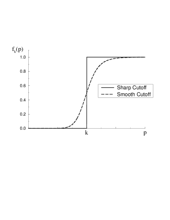
FIG. 1.: The sharp blocking function (solid line) and a typical smooth blocking function (dashed line).

FIG. 2.: The real part of the RG–improved effective potential $U_{\beta,k=0}(v)$ for different values of the temperature. The phase transition is clearly second order.

FIG. 3.: The effective chemical potential $\mu_{\beta,k=0}$ and the effective quartic coupling $g_{\beta,k=0}$ near the critical temperature. Both vanish at $T_{c}$.

FIG. 4.: The critical exponent $\nu$ as a function of number of terms, $N$, in the polynomial expansion.

FIG. 5.: The critical exponent $\nu$ as a function of the smoothing parameter $m$ for different values of the number of terms, $N$, in the polynomial expansion.

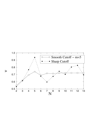
FIG. 6.: The critical exponent $\nu$ as function of the number of terms, $N$, in the polynomial expansion using a sharp cutoff and a smooth cutoff with $m=5$.

REFERENCES

- [1] M. H. Anderson, J. R. Ensher, M. R. Matthews, C. E. Wieman and E. A. Cornell, Science 269, 198, 1995.
- [2] K. B. Davis, M. O. Mewes, M. R. Andrews, N. J. van Druten, D. S. Durfee, D. M. Kurn and W. Ketterle, Phys. Rev. Lett 75, 3969, 1995.
- [3] C. C. Bradley, C. A. Sackett, J. J. Tollet and R. G. Hulet, Phys. Rev. Lett. 75, 1687, 1995.
- [4] F. Dalfovo, S. Giorgini, L. P. Pitaevskii and S. Stringari, cond–mat/9806038. Phys. Rev. Lett. 75, 1687, 1995.
- [5] C. J. Pethick and H. Smith, “Bose-Einstein Condensation in Dilute Gases”, Nordita lecture notes, September 1997.
- [6] T.D. Lee and C.N. Yang, Phys. Rev. 105, 1119 (1957); T.D. Lee, K. Huang, and C.N. Yang, Phys. Rev. 106, 1135 (1957); C.N. Yang, Physica 26, 549 (1960).
- [7] T.T. Wu, Phys. Rev. 115, 1390 (1959); N.M. Hugenholtz and D. Pines, Phys. Rev. 116, 489 (1959); K. Sawada, Phys. Rev. 116, 1344 (1959).
- [8] E. Braaten and A. Nieto, Phys. Rev. B 56, 14745, 1997.
- [9] J. Zinn–Justin, Quantum field Theory and Critical Phenomena, Oxford University Press Inc., New York, 1989.
- [10] A. Griffin, Physica. C 156, 12, 1988.
- [11] M. Bijlsma and H. T. S. Stoof, cond–mat/9603029.
- [12] T. Haugset, H. Haugerud and F. Ravndal, Ann. Phys. 226, 27, 1998.
- [13] K. Wilson and J. Kogut, Phys. Rep. 12, 75, 1974.
- [14] J. Polchinski, Nucl. Phys. B 231, 269,1984.
- [15] D.S. Fisher and P.C. Hohenberg, Phys. Rev. B 37, 4936 (1988).
- [16] P.B. Weichmann, Phys. Rev. B 38, 8739 (1988).
- [17] E.B. Kolomeisky and J.P. Straley, Phys. Rev. B 46, 11749 (1992).
- [18] E.B. Kolomeisky and J.P. Straley, Phys. Rev. B 46, 13942 (1992).
- [19] M. Bijlsma and H. T. S. Stoof, Phys. Rev. A 54, 5085, 1996.
- [20] H. Shi and A. Griffin, “Finite Temperature Excitations in a Dilute Bose-condensed Gas”, to appear in Physics Reports.
- [21] P. Arnold and L. G. Yaffe, Phys. Rev. D 49, 3003, 1994.
- [22] T. R. Morris, Phys. Lett B 334, 355, 1994; Nucl. Phys. B 509, 637, 1998.
- [23] K.–I. Aoki, K. Morikawa, W. Souma, J.–I. Sumi and H.Terao, Prog. Theor. Phys. 99, 451, 1998.
- [24] N. Tretradis and C. Wetterich, Nucl. Phys. B 422, 541, 1994.
- [25] R. D. Ball, P. E. Haagensen, J. I. Torre and E. Moreno, Phys. Lett. B 347, 80, 1995.
- [26] S.–B. Liao and M. Strickland, Nucl. Phys. B 497, 611, 1997.
- [27] Eric Braaten, hep-ph/9809405.
- [28] H. Georgi, Ann. Rev. Nucl. Part. Sci. 43, 209, 1993; E. Braaten and A. Nieto, Phys. Rev. B 55, 8090, 1997.
- [29] S.–B. Liao and M. Strickland, Phys. Rev. D 52, 3653, 1995.
- [30] P. C Hohenberg and and P. C. Martin, Ann. Phys. 34, 291, 1965.
- [31] M. Gell-Mann and K. A. Brückner, Phys. Rev 106, 364, 1957.
- [32] M. D’Attanasio and M. Pietroni, Nucl. Phys. B 472, 711, 1996.
- [33] B. Bergerhoff, Phys.Lett. B 437, 381, 1998; B. Bergerhoff and J. Reingruber, cond-mat/9809251.
- [34] A. J. Niemi and G. W. Semenoff, Ann. Phys. 152, 105, 1984.
- [35] S.-B. Liao and M. Strickland, Nucl.Phys. B 532, 753, 1998.
- [36] T. Morris, Int. J. Mod. Phys. B 12, 1343, 1998.
- [37] N. P. Landsman. Nucl. Phys. B 322, 498, 1989.
- [38] J. F. Nicoll, T. S. Chang and H. E. Stanley, Phys. Rev. Lett. 33, 540, 1974.