Transition from the Compact to the Dense Phase of Two-Dimensional Polymers

Abstract

We present a unifying picture of the compact, dense and dilute phases of two-dimensional polymers. The lattice dependence of the scaling exponents for compact polymers is reconciled with their universality in the dense and dilute case. In particular, we show that violations of the fully-packing constraint in the compact phase can be interpreted as magnetic screening in the associated Coulomb gas, which induces a flow to either the dense or the dilute phase. When more than one flavour of polymers is present the flow away from the compact phase leads to a decoupling of the flavours, and the central charge decreases by an integer. If charge asymmetry develops the polymer flavours may independently flow to either of the two non-compact phases.

I Introduction

Unlike polymers in the much studied dense and dilute phases [1], two-dimensional polymers in the compact phase exhibit a remarkable lack of universality. Namely, their scaling properties are described by conformal field theories that depend crucially on the coordination number of the underlying lattice. This leads to an unusual situation where critical exponents for compact polymers on the square and the honeycomb lattice are different [2, 3, 4, 5, 6].

Another intriguing property of compact polymers, which by definition cover all the lattice sites, is that they constitute new universality classes that differ from that of dense polymers [7], for which the fraction of covered sites $0<f<1$. In the dilute phase, which corresponds to a polymer in a good solvent, $f=0$.

The difference between compact and dense polymers is easily understood from the random surface perspective. Namely, two-dimensional polymers can be mapped to a lattice model of a fluctuating interface which is described in the scaling limit by a Liouville field theory with imaginary couplings. However, whilst the dense and dilute phases are both adequately described by a scalar height, the fully-packing (or Hamiltonian) constraint imposed on compact polymers forces the height space to be $(z-1)$-dimensional, $z$ being the coordination number of the lattice at hand. The larger dimensionality of the height space leads to a more complicated effective field theory and to new exponents [4, 6].

Nonetheless, certain critical exponents turn out to be “super-universal”, in the sense that they are identical for dense polymers and compact polymers on the square and honeycomb lattice. Consider the exponents $x_{s}$, for $s=1,2,\ldots$, governing the power-law decay of the correlation function $G_{s}(r)\sim r^{-2x_{s}}$ which describes $s$ polymer chains with one end anchored within a small region centred around the origin, and the other in a region around a distant point ${\bf r}$. A comparison of the explicit expressions for these so-called string (or watermelon) dimensions for the three models under consideration reveals that they are the same for $s$ even. This is also true of the difference $x_{s}-x_{s^{\prime}}$ between any two odd string dimensions. These observations have important consequences for the physically relevant contact exponents $\theta_{\cal G}$. These exponents determine the asymptotic decay of the probability $P_{\cal G}(y)\sim y^{\theta_{\cal G}}$ as $y\to 0$, that a certain number of points on the polymer separated by macroscopic distances along the chain, simultaneously have a spatial separation of order $y$; the arrangement of contact points is specified by the graph ${\cal G}$. Restricting for simplicity the attention to two-point contacts, it is easily seen that $\theta_{\cal G}$ only depends on the string dimensions through the universal combinations $x_{3}-x_{1}$ and $x_{4}$, as long as only interior points and at most one of the endpoints of the polymer are involved in the contact. On the other hand, contacts involving both endpoints give rise to exponents that depend on $x_{1}$ separately, and hence are not universal. Incidentally, $x_{1}$ also determines the conformational exponent $\gamma=1-x_{1}$, which describes the scaling of the ratio of the number of open to closed polymer chains with their length, and is a measure of the effective entropic interaction between the two polymer ends. For compact polymers on the honeycomb lattice the mean-field [9] result $x_{1}^{\rm ch}=0$ was found [3, 4], whereas both compact polymers on the square lattice and dense polymers exhibit an effective entropic repulsion between chain ends with $x_{1}^{\rm cs}=-5/112$ and $x_{1}^{\rm d}=-3/16$ respectively [6, 7].

This paper aims at providing a theory of the transition from the compact to the dense phase, with emphasis on the mechanism that restores the universality of the string dimensions when violations of the fully-packing constraint are permitted. A particularly interesting framework for these investigations is an extension of the square-lattice model which was used to solve the compact polymer problem in Ref. [6]. Namely, this model allows for the definition of two mutually excluding flavours (species) of polymers, which in the compact case were found to interact in a manner that endowed the model with a two-dimensional manifold of critical fixed points. Apart from the obvious interest in examining what happens to the Liouville field theory as one flows away from the compact phase, it is a most beguiling question whether the dense and dilute phases also allow for a two-flavour extension. We shall find the answer to this question to be affirmative, with an important caveat: Once vertices are allowed to be uncovered by the polymers, the two flavours decouple. Quite remarkably, this decoupling turns out to be so complete that one of the flavours may even flow to the dilute phase whilst the other remains dense! This provides a rationalisation for four of the five critical branches of the O($n$) model studied in Ref. [10].

We begin (in Section II) by giving a heuristic argument, based on the field theory for the compact phase, that explains how dense exponents may emerge from the compact ones when we allow for violations of the $f=1$ constraint. In the Coulomb gas formalism string dimensions such as the ones defined above are determined by inserting a pair of electromagnetic test charges into the vacuum, and calculating their interaction energy. Violations of the compactness constraint are shown to correspond to magnetic charges which form a plasma that completely screens one of the components of the vector magnetic charge of the test particles. As a result the compact string dimensions reduce to those of two non-interacting flavours of dense polymers.

Though physically appealing this argument is unsound. We therefore go on (in Section III) to propose a lattice model that exhibits all three phases of polymers—compact, dense, and dilute. Exact values of the central charge and the critical exponents are then computed from a Coulomb gas construction which, although not mathematically rigorous, is well founded in the renormalisation group [1]. These results neatly confirm the more intuitive magnetic plasma picture, and go further in describing the interplay between the dense and dilute phase.

Even though the two-flavoured model on the square lattice is our prime concern, the ideas presented here are quite general. In particular they apply to the one-flavoured model on the honeycomb lattice, and in general to loop models defined on arbitrary $z$-fold coordinated regular lattices. This is the subject of the Discussion (Section IV), where we also elaborate on the relation between our results and those obtained for the O($n$) model of Ref. [10].

II Coulomb gas with a magnetic plasma

A Two-flavour fully packed loop model

In Ref. [6] scaling properties of compact polymers on the square lattice were investigated with the help of the two-flavour fully packed loop (FPL²) model. This model has a two-dimensional region of critical fixed points wherein compact polymers are identified with a single point; this point also belongs to a line of fixed points which is a subset of the critical manifold and it describes interacting compact polymers. Since our results for the compact-to-dense transition extend to the entire critical manifold we shall begin by briefly reviewing the FPL² model.

First define ${\cal G^{\prime}}$ to be the set of all edge colourings of the square lattice with four different colours. In other words, each edge of the lattice is assigned a colour ${\bf A}$, ${\bf B}$, ${\bf C}$ or ${\bf D}$, subject to the constraint that for any vertex all of its four adjacant edges carry different colours. If we bipartition the square lattice into even and odd sublattices, directed loops of two different flavours (“black” and “grey”) can be defined as follows: Colour ${\bf A}$ designates a black loop segment directed from an even to an odd site, and colour ${\bf B}$ corresponds to a black loop segment having the opposite direction. Similarly colours ${\bf C}$ and ${\bf D}$ are used to define directed grey loops. By ${\cal G}$ we denote the equivalence classes of ${\cal G^{\prime}}$ with respect to independent changes of directions for each of the loops. The FPL² partition function is then

$$Z=\sum_{\cal G}n_{\rm b}^{N_{\rm b}}n_{\rm g}^{N_{\rm g}}\ ,$$ (1)

where $n_{\rm b},n_{\rm g}$ are the fugacities and $N_{\rm b},N_{\rm g}$ the numbers of (undirected) black and grey loops in ${\cal G}$ respectively. The model (1) is critical on the manifold $0\leq n_{\rm b},n_{\rm g}\leq 2$, and the compact polymer problem discussed in the Introduction is recovered in the limit $(n_{\rm b},n_{\rm g})\to(0,1)$.

The extra orientational information present in ${\cal G^{\prime}}$ allows for a local redistribution of the loop fugacities. Indeed, assign a phase factor $\exp(\pm{\rm i}\pi e_{\rm b}/4)$ to each vertex where a directed black loop makes a right (left) turn, and the factor $1$ if it continues straight. In this way the weight of the entire black loop becomes $\exp(\pm{\rm i}\pi e_{\rm b})$ if the orientation is clockwise (counter-clockwise). The undirected loop weight $n_{\rm b}$ is obtained by summing over the two orientations, whence $n_{\rm b}=2\cos(\pi e_{\rm b})$. With a similar convention for the grey loops, and letting $\lambda({\bf x})$ be the product of the local black and grey weights at the vertex ${\bf x}$, the partition function, Eq. (1), can now be rewritten as

$$Z=\sum_{{\cal G^{\prime}}}\prod_{{\bf x}}\lambda({\bf x})\ .$$ (2)

The continuum limit of the FPL² model is obtained by mapping the oriented loop configurations to an interface model defined on the dual lattice. The microscopic heights ${\bf z}$ live on the plaquettes of the square lattice and they are defined, up to an overall shift, by the edge colours which stipulate the height differences between neighbouring plaquettes. More precisely, when encircling an even (odd) site in the clockwise direction a vector ${\bf A}$, ${\bf B}$, ${\bf C}$ or ${\bf D}$ is added to (subtracted from) ${\bf z}$ depending on the state of the edge being crossed. The fully-packing constraint imposes the condition

$${\bf A}+{\bf B}+{\bf C}+{\bf D}={\bf 0}\ ,$$ (3)

whence the colour vectors are three-dimensional. A suitable representation is

$${\bf A}=(-1,+1,+1)\ ,\ \ \ \ {\bf B}=(+1,+1,-1)\ ,$$ (4)

$${\bf C}=(-1,-1,-1)\ ,\ \ \ \ {\bf D}=(+1,-1,+1)\ .$$ (5)

The continuum limit is then taken by coarse graining ${\bf z}$. The effective field theory is described by a Liouville action containing three terms [11]:

$$S=S_{\rm E}+S_{\rm B}+S_{\rm L}\ .$$ (6)

The elastic part $S_{\rm E}$ is a gradient-squared term in the coarse grained height ${\bf h}({\bf x})$, and it controls the fluctuations of the interface away from flat configurations. The boundary term $S_{\rm B}$ assigns the correct weights to loops winding around the point at infinity by coupling ${\bf h}$ to the scalar curvature $\tilde{\cal R}$. Finally, $S_{\rm L}$ is a Liouville potential that assigns the correct weights to loops in the bulk, and it is the coarse grained version of the microscopic vertex weights $\lambda({\bf x})$.

In the dual Coulomb gas picture the action, Eq. (6), is interpreted as that of a two-dimensional gas of electro-magnetic vector charges interacting via a logarithmic potential. Electric charges are associated with vertex operators $\exp({\rm i}{\bf e}\cdot{\bf h})$ which appear as the scaling limits of FPL² operators that can be expressed as local, periodic functions of the microscopic heights. Magnetic charges ${\bf m}$ act as non-local constraints on the height field, and they are associated with topological defects in the microscopic heights or, equivalently, with violations of the four-colouring constraint. Finally, the curvature term $S_{\rm B}$ introduces a background electric charge $-2{\bf e}_{0}$ at the boundary of the system. For reasons of neutrality this endows the Coulomb gas vacuum with a floating charge $+2{\bf e}_{0}$ located in the bulk of the system.

B Height defects and magnetic screening

Following the standard Coulomb gas recipe [1], the calculation of the scaling dimension of an electromagnetic operator reduces to the determination of the interaction energy of “test particles” of charge $\pm({\bf e},{\bf m})$ inserted into the vacuum. This energy varies logarithmically with separation, where the prefactor of the logarithm is twice the sought dimension. As the floating charge is free to move around the bulk it will coalesce with one of the test particles thus minimising the energy. Therefore the interaction energy consists of three terms associated with the pairwise interactions of the background electric charge $(-2{\bf e}_{0},0)$, $({\bf e},{\bf m})$, and $(2{\bf e}_{0}-{\bf e},-{\bf m})$, with the vacuum energy subtracted off. The energy of the vacuum is simply due to the pair interaction between the background charge and the floating charge.

Consider, for example, the computation of the string dimensions $x_{s}$ for the FPL² model. Since the defect strings may now have any of the two flavour labels this generalises to $x_{s_{\rm b},s_{\rm g}}$, where $s_{\rm b}$ ($s_{\rm g}$) denotes the number of black (grey) strings. For dislocations generated in the bulk the number $s_{\rm b}+s_{\rm g}$ must be even [6]. Appropriate defect configurations may be specified through the colouring state of the four edges around some fixed vertex [12]. For instance, $({\bf A},{\bf A},{\bf C},{\bf D})$ generates two directed black strings and corresponds to a height vortex of strength ${\bf m}_{2,0}={\bf A}-{\bf B}=(-2,0,2)$. Similarly, $({\bf A},{\bf B},{\bf C},{\bf C})$ is a vortex of strength ${\bf m}_{0,2}={\bf C}-{\bf D}=(-2,0,-2)$ that generates two grey strings, and $({\bf A},{\bf C},{\bf C},{\bf D})$ generates one string of either flavour and has strength ${\bf m}_{1,1}={\bf C}-{\bf B}=(-2,-2,0)$. For simplicity we shall concentrate on the black strings and define $x_{s}=x_{s,s_{\rm g}}$, where $s_{\rm g}=s\mbox{ mod }2$. The defect magnetic charge

$${\bf m}_{s}=\left\{\begin{array}[]{ll}(-s,0,s)&\mbox{for $s$ even,}\\ (-s-1,-2,s-1)&\mbox{for $s$ odd,}\end{array}\right.$$ (7)

found as a suitable linear combination of ${\bf m}_{2,0}$ and ${\bf m}_{1,1}$, must be accompanied by an appropriate compensating electric charge that takes care of the spurious phase factors arising from the winding of the strings around the defect cores [1]. Setting the fugacity of the grey strings equal to unity ($e_{\rm g}=1/3$) we obtain the following result for the scaling dimensions:

$$2x_{s}=\left\{\begin{array}[]{ll}\frac{1}{4}(1-e_{\rm b})s^{2}-\frac{e_{\rm b}^{2}}{1-e_{\rm b}}&\mbox{for $s$ even,}\\ \frac{1}{4}(1-e_{\rm b})s^{2}-\frac{e_{\rm b}^{2}}{1-e_{\rm b}}+\frac{2(1-e_{\rm b})}{5-3e_{\rm b}}&\mbox{for $s$ odd.}\end{array}\right.$$ (8)

As mentioned in the Introduction the even scaling dimensions agree with those of dense polymers [7] (and also with those of the fully-packed loop model on the honeycomb lattice [4]), whereas the odd dimensions contain an extra term due to the coupling between the black and the grey strings.

So far our discussion has been for the fully-packed case where a fraction $f=1$ of the lattice vertices are visited by both loop flavours. Now consider moving infinitesimally into the dense phase by diminishing the fraction of visited vertices to $f=1-\epsilon$. One can imagine doing so by distributing a fraction $\epsilon$ of $({\bf A},{\bf B},{\bf A},{\bf B})$ defects and a fraction $\epsilon$ of $({\bf C},{\bf D},{\bf C},{\bf D})$ defects throughout the system. The corresponding vortices have magnetic charge $\pm{\bf m}_{T}$, where

$${\bf m}_{T}=(0,4,0)\ .$$ (9)

Physically this situation corresponds to having a dilute magnetic plasma superimposed on the Coulomb gas vacuum.

As before we can then imagine inserting two electromagnetic test particles of charge $\pm({\bf e},{\bf m})$ into the system in order to measure the string scaling dimensions. Just as in the familiar case of electric test particles in a dielectric medium there will now be some screening, the difference being that here it is the magnetic charge that is being screened. However, unlike what is the case in this dielectric analogy, the magnetic plasma is completely free to move around, and the screening will be complete. This is a consequence of the fact that the magnetic charges in Eq. (9) are relevant, i.e. their scaling dimension [6]

$$2x(\pm{\bf m}_{T})=4\ \frac{(1-e_{\rm b})(1-e_{\rm g})}{(1-e_{\rm b})+(1-e_{\rm g})}$$ (10)

is less than 2 on the whole critical manifold of the FPL² model. Therefore these charges are not bound into vortex-antivortex pairs at large scales [13].

Taking our cue from this intuitive picture we hypothesise that the effect of the magnetic plasma can be modeled by the substitution

$${\bf m}\equiv(m^{1},m^{2},m^{3})\longrightarrow{\bf m}^{\prime}\equiv(m^{1},0,m^{3})\ ,$$ (11)

since the only non-vanishing component of the screening charge (9) is along the 2-direction, and this does not couple to any of the other directions. In particular, replacing ${\bf m}_{s}$ of Eq. (7) by ${\bf m}_{s}^{\prime}$ we find that instead of Eq. (8) we get

$$2x_{s}^{\prime}=\frac{1}{4}(1-e_{\rm b})s^{2}-\frac{e_{\rm b}^{2}}{1-e_{\rm b}}$$ (12)

for all $s$, whether even or odd! It seems that the interaction between the two loop flavours that was responsible for the difference between the even and odd string dimensions in Eq. (8) has somehow been disposed of, and what remains is the critical exponents of dense polymers [7].

One can proceed to compute the central charge for the screened system. We recall that in the compact ($f=1$) case this was given as $c=3+12x({\bf e}_{0},{\bf 0})$, where the three free bosons present in $S_{\rm E}$ each contribute unit central charge, and there is a negative shift due to the background electric charge. However, since the magnetic charges live in height space the complete screening of $m^{2}$ means that height fluctuations along the 2-direction are frozen out. This is nothing but the usual Kosterlitz-Thouless scenario [13], where due to the unbinding of dislocations the interface defined by the second height component is rendered smooth. As a result the central charge for $f=1-\epsilon$ is $c^{\prime}=c-1=2+12x({\bf e}_{0},{\bf 0}^{\prime})$, which can be written as

$$c^{\prime}(e_{\rm b},e_{\rm g})=c^{\rm dn}(e_{\rm b})+c^{\rm dn}(e_{\rm g})\ ,$$ (13)

where

$$c^{\rm dn}(e)=1-\frac{6e^{2}}{1-e}$$ (14)

is nothing but the central charge of one flavour of dense polymers [7]. If we again set the fugacity of the grey loops equal to unity ($e_{\rm g}=1/3$) we find that $c^{\rm dn}(e_{\rm g})=0$, and only the contribution from the black loops remains. The sum rule (13) should be taken as a further indication that once we allow for violations of the fully-packing constraint the two loop flavours decouple.

At this point, of course, a number of objections may be raised. First, it is seen from Eq. (7) that the magnitude of the magnetic charge along the 2-direction is $-2$. However, for the screening to take place it then seems that the magnetic screening charges $\pm{\bf m}_{T}$ given by Eq. (9) must somehow be fractionalised.

Another objection is that the above calculation, when taken at face value, purports to be perturbative around the fully-packed phase. However, as pointed out earlier [Eq. (10)] the defect operators within the FPL² model are strongly relevant! This means that the fugacity of these defects will flow off to infinity at large scales. Hence, the magnetic plasma analogy is no more than a heuristic argument. Nevertheless, we shall see in the following section that it is possible to generalise the FPL² model to a lattice model that explicitly accommodates configurations that are not fully packed. In this generalised model Coulomb gas calculations can be carried out, confirming the main results found in this Section.

Even when accepting the magnetic plasma analogy as a heuristic framework for treating the case of $f<1$, the FPL² height mapping on which it is based breaks down completely for $f\to 0$. It is therefore impossible to say anything about the role of the dilute polymer phase. However, from the calculations presented in the next Section we shall be able to say more about how dilute exponents may emerge.

III Two-flavour densely packed loop model

In order to unify our understanding of compact, dense and dilute polymers as well as their possible interrelation we introduce a statistical mechanics model that can accommodate all three phases. Since the critical properties of the compact phase are known to be lattice dependent we need to consider the model on a specific lattice. To examine the important issues associated with the presence of more than one loop flavour we choose the square lattice, whereas the question of what the construction would look like on other lattices is deferred to the Discussion.

FIG. 1.: The ten allowed vertices in the DPL² model. Black and grey loop segments are represented by solid and dashed linestyle respectively.

We therefore define the two-flavour densely packed loop (DPL²) model on the square lattice by listing its ten allowed vertex states in Fig. 1. The first six vertices are those familiar from the fully packed (FPL²) case, whilst the last four vertices explicitly allow the model to violate the fully-packing constraint. Vertices 7–8 exclude the grey loops from a given site and carry a weight $W_{\rm b}$, and similarly vertices 9–10 exclude the black loops and have weight $W_{\rm g}$. The first six vertices are all assigned unit weight. The partition function of the DPL² model is then

$$Z=\sum_{{\cal G}^{\rm d}}W_{\rm b}^{v_{\rm b}}W_{\rm g}^{v_{\rm g}}n_{\rm b}^{N_{\rm b}}n_{\rm g}^{N_{\rm g}}\ ,$$ (15)

where $n_{\rm b},n_{\rm g},N_{\rm b},N_{\rm g}$ have the same meaning as in Eq. (1), and $v_{\rm b}$ and $v_{\rm g}$ are the number of occurrences of vertices 7–8 and 9–10, respectively. The summation runs over the set ${\cal G}^{\rm d}$ of loop configurations on the square lattice that can be made out of vertices 1–10, subject to the constraint that both flavours form closed loops. This model is closely related to the O($n$) model introduced in Ref. [10] for which five branches of critical points were found as a function of $n$. In the Discussion we shall comment on the precise relation of the DPL² model to this one, thus providing a physical picture of its critical properties.

Clearly, in the special case $(W_{\rm b},W_{\rm g})=(0,0)$ the DPL² model reduces to the FPL² model, and the analysis of Ref. [6] applies. Let us briefly recall the main results of this fully packed case. For $s_{\rm b}+s_{\rm g}=0\mbox{ mod }2$ the full spectrum of string dimensions is

$$2x_{s_{\rm b},s_{\rm g}} = \frac{1}{4}\left[(1-e_{\rm b})s_{\rm b}^{2}+(1-e_{\rm g})s_{\rm g}^{2}\right]$$ (16)

$$- \left[\frac{e_{\rm b}^{2}}{1-e_{\rm b}}(1-\delta_{s_{\rm b},0})+\frac{e_{\rm g}^{2}}{1-e_{\rm g}}(1-\delta_{s_{\rm g},0})\right]$$ (17)

$$+ \delta^{(2)}_{s_{\rm b},1}\delta^{(2)}_{s_{\rm g},1}\frac{(1-e_{\rm b})(1-e_{\rm g})}{(1-e_{\rm b})+(1-e_{\rm g})},$$ (18)

where $\delta^{(2)}_{i,j}\equiv\delta_{i=j\rm{(mod\ 2)}}$. The result for the central charge is

$$c=3-6\left(\frac{e_{\rm b}^{2}}{1-e_{\rm b}}+\frac{e_{\rm g}^{2}}{1-e_{\rm g}}\right)\ .$$ (19)

In the following we focus on the Coulomb gas construction for the case where either $W_{\rm b}$ or $W_{\rm g}$ is greater than zero.

A Colouring and height representation

The mapping from oriented loop configurations ${\cal G^{\prime}}^{\rm d}$ to the four-colouring representation goes through exactly as described for the FPL² model in Sec. II A. When defining the microscopic heights ${\bf z}$ there is however one very important difference. The presence of vertices 7–10 in Fig. 1 imposes extra constraints on the choice of the colour vectors:

$${\bf A}+{\bf B}={\bf 0}\ ,\ \ \ \ {\bf C}+{\bf D}={\bf 0}\ .$$ (20)

Actually, whenever one of these constraints holds true the other follows from Eq. (3). So the conditions (20) are valid provided that either $W_{\rm b}>0$ or $W_{\rm g}>0$.

As a consequence the color vectors in Eq. (5) must be replaced by

$${\bf A}=(+1,0),\ \ \ \ {\bf B}=(-1,0),$$ (21)

$${\bf C}=(0,+1),\ \ \ \ {\bf D}=(0,-1),$$ (22)

i.e., the height space is now two-dimensional. This elimination of one of the height components is very reminiscent of the effect of screening in the magnetic plasma analogy of Sec. II.

The local redistribution of the loop fugacities, $n_{\rm b}$ and $n_{\rm g}$ of Eq. (15), in terms of local weight factors associated with the left and right turns of the loops, again takes place as in Sec. II A. One may wonder how should the vertex weights $W_{\rm b}$ and $W_{\rm g}$ be represented? Unlike the loop weights which do not renormalise under a change of scale, the vertex weights do change under scale transformations as they flow towards their fixed-point (and non-universal) values. Thus, from the point of view of the Liouville field theory description that we are about to set up for the scaling limit, they need not be represented at all! Of course, all along our working assumption is that the scaling limit of the DPL² model exists for loop fugacities $0\leq n_{\rm b},n_{\rm g}\leq 2$ .

B Ideal states

An ideal state of a loop model has two distinguishing features. First, it is macroscopically flat, so that fluctuations of the interface around the ideal states can be controlled by an elastic term $S_{\rm E}$ in the effective action. Second, it is entropically selected in the sense that it maximises the number of configurations which differ from it by the smallest allowed change. To be concrete consider the directed FPL² model in the four-colouring representation. Since any change of a configuration must necessarily involve the change of some edge colour $\sigma_{1}$ into another colour $\sigma_{2}$, it follows that the whole loop $\sigma_{1}\sigma_{2}\sigma_{1}\sigma_{2}\cdots\sigma_{1}\sigma_{2}$ defined as an alternating sequence of these two colours must be changed into $\sigma_{2}\sigma_{1}\sigma_{2}\sigma_{1}\cdots\sigma_{2}\sigma_{1}$. An ideal state allows for the maximum number of such loop flips, and consequently has a maximum number of small loops of alternating colour.

FIG. 2.: Representative examples of ideal states in the FPL² model, here shown in the oriented loop representation. The full ideal state is obtained by tiling $\sf I\hskip-1.5ptR^{2}$ with the $2\times 2$ pattern given in the figure. Each of the examples corresponds to a group of eight ideal states, related by independent changes of orientations for the two flavours, and by flavour conjugation.

In the FPL² model on the square lattice there are 24 ideal states, defined by the 4! possible permutations of the colours ${\bf A}$, ${\bf B}$, ${\bf C}$ and ${\bf D}$ around a fixed vertex. For later convenience we choose to label them by the clockwise sequence $(\sigma_{1},\sigma_{2},\sigma_{3},\sigma_{4})$ of colours around this vertex, starting with the leftmost edge. In the oriented loop representation the ideal states form a pattern of $2\times 2$ plaquettes which is repeated throughout the lattice. Three representative examples are shown in Fig. 2.a–c. Taking into account the possible changes of loop flavours and directions there are eight FPL² ideal states corresponding to each of these examples, making a total of 24.

When we allow for the extra vertices of the DPL² model more ideal states become possible. Namely, for each of the 16 states exemplified by Fig. 2.a–b there corresponds another ideal state where only one of the two loop flavours is used to form the small loops. Again we can label the states by means of the colour configuration around a fixed vertex, but as shown in Fig. 3 this is in some cases no longer unique. To remedy this we adopt the convention to add a prime to the label whenever the loop configuration around a vertex is as shown in Fig. 2.a; see Fig. 3.

FIG. 3.: Certain colour configurations around a vertex do not uniquely specify the directed loop configuration. In particular the label $({\bf B},{\bf A},{\bf B},{\bf A})$ corresponds to two distinct DPL² ideal states, which we distinguish by a prime as shown.

This ambiguity has also bearings on the way in which changes of a given colouring configuration may be performed. Namely, when changing some edge colour $\sigma_{1}$ into $\sigma_{2}$ one may encounter one of the ambiguous vertices of Fig. 3 in the process of tracing out the loop $\sigma_{1}\sigma_{2}\sigma_{1}\sigma_{2}\cdots\sigma_{1}\sigma_{2}$ to be flipped. In that case one has two equivalent choices for proceding. However, this peculiarity does not change the fact that the 16 new states are still ideal, since they are perfectly macroscopically flat and they allow for an equal number of small changes as do the 24 ideal states of the FPL² model. The DPL² model thus has 40 ideal states.

The lesson to be learned from this complication is that it is favourable to think of the DPL² ideal states in terms of the oriented loop representation rather than in terms of the colouring representation. In fact, the mapping from oriented loop configurations to the four-colouring representation is now many-to-one, so that the inverse mapping is no longer well-defined. Since we only need the colours to define the heights, which are the basic constituents of the continuum field theory, we do not have to worry whether the series of mappings can be reversed.

C More on the dimensionality of height space

It is worthwhile noticing that the choice (22) would have been just as good as (5) in ensuring the one-to-one correspondence between oriented FPL² configurations and the microscopic heights. However, a too restrictive choice of the colour vectors may render a non-ideal state macroscopically flat, in which case the elastic term $S_{\rm E}$ of the action fails to enforce the proper entropic penalty for a state that does not allow for a maximum number of loop flips.

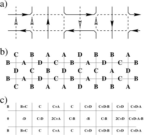
FIG. 4.: This FPL² state has a non-vanishing macroscopic height gradient along the horizontal direction. It is shown in three equivalent representations: (a) oriented loops, (b) edge colourings, and (c) microscopic heights.

As an example consider the state arising from a tiling of $\sf I\hskip-1.5ptR^{2}$ with the $2\times 8$ pattern shown in Fig. 4. Upon coarse graining this state is flat in the vertical ($x^{2}$) direction, but has a macroscopic height gradient in the horizontal direction:

$$\partial{\bf h}/\partial x^{1}=\frac{1}{8}\>[({\bf C}+{\bf D})-({\bf A}+{\bf B})]\ .$$ (23)

With the choice (22) the height gradient vanishes, and $S_{\rm E}=0$ for this height configuration. On the other hand, the choice (5) leads to $\partial{\bf h}/\partial x^{1}=(0,-1/2,0)$, and the state is duly suppressed by $S_{\rm E}$ since the stiffness constant along the second height direction

$$K_{22}=\frac{(1-e_{\rm b})(1-e_{\rm g})}{(1-e_{\rm b})+(1-e_{\rm g})}$$ (24)

is non-zero throughout the critical region [6].

This important point is further illuminated by noting that black and grey loops play the role of contour lines for the projection of ${\bf h}$ along the $(1,0,-1)$ and the $(1,0,1)$ directions respectively. Evidently these projections fail to detect any variation along the 2-direction in height space, and accordingly the state given by Fig. 4 appears macroscopically flat when viewed exclusively in terms of its oriented loop representation.

D Ideal state graph

The 40 ideal states of the DPL² model define the ideal state graph ${\cal I}$ which is instrumental in the construction of the continuum field theory. The idea is to identify the ideal states with nodes on ${\cal I}$ whose position is given by the average microscopic height $\langle{\bf z}\rangle$ of the given state. Two ideal states are said to be nearest neighbours if their respective microscopic heights are identical on three fourths of the lattice plaquettes. On ${\cal I}$, the two nodes corresponding to such a nearest neighbour pair are connected through a link.

FIG. 5.: Ideal state graph ${\cal I}$ of the DPL² model. The thick and thin linestyles distinguish the links which are inherited from the FPL² model from those which are new to the DPL² model. The scale is set by the squares in thick linestyle, which have side length $1/2$.

The result of this construction is the ideal state graph shown in Fig. 5. Here the links added due to the inclusion of the 16 ideal states which are new to the DPL² model are shown as thin lines, whereas the thick linestyle designates links between the 24 ideal states which have been inherited from the FPL² model. We recall that the ideal state graph for the FPL² model was a covering of $\sf I\hskip-1.5ptR^{3}$ by truncated octahedra. Since the DPL² colour vectors (22) can be obtained from their FPL² counterparts (5) by a projection onto the $z^{1}z^{3}$-plane and a subsequent $\frac{3\pi}{4}$ rotation and rescaling, it should hardly come as a surprise that the thick lines form a two-dimensional projection of the truncated octahedra. In particular, the square and the hexagonal faces are clearly visible.

FIG. 6.: The repeating unit of ${\cal I}$ along with the state labels. Ideal states that are new to the DPL² model can easily be distinguished by noting that only two different colour vectors appear in their state label.

As a consequence of our definition of nearest neighbour ideal states any one ideal state corresponds to an infinity of nodes in ${\cal I}$. The entire ideal state graph thus corresponds to a covering of $\sf I\hskip-1.5ptR^{2}$ by the repeating unit shown in Fig. 6. Two novel features of the DPL² ideal state graph which have not been encountered in the previously studied loop models are that each node may have several labels, and that links may cross without being connected by a node. The latter observation just indicates that ${\cal I}$ really must be thought of as a graph (a collection of nodes and links) and not simply a lattice; of course, unlike the usual notion of a graph, the precise location of the nodes is of paramount importance as it bears on the effective field theory of the model.

Concentrating first on the 24 ideal states on Fig. 6 that are connected by thick links the division of the states into the three classes exemplified by Fig. 2 becomes obvious. The two groups of eight states having the elementary plaquette loops positioned as on Fig. 2.a and Fig. 2.b respectively, each form a square with doubly labeled nodes. These squares are connected by thick lines via two four-fold labeled nodes (“crosses” on Fig. 6) that together accommodate the eight states of the type shown in Fig. 2.c. The remaining 16 ideal states which are new to the DPL² model, located at intersections of thin lines in Fig. 6, occur in two groups of eight states corresponding to plaquette loops positioned as in Fig. 2.a (primed states) and in Fig. 2.b (unprimed states). Quite naturally, the primed states are linked to the square of eight FPL² states with loops positioned as shown in Fig. 2.a, and similarly the unprimed states are distributed around the other square (cfr. Fig. 2.b). In particular, the states ${\bf DCDC}$ and ${\bf DCDC}^{\prime}$ must be thought of as labeling two distinct nodes, which just happen to occupy identical positions on Fig. 6. This subtlety becomes more evident if one tries to trace out ${\cal I}$ explicitly by moving from one ideal state to the neighbouring one. This is accomplished by either choosing two colours in the starting ideal state and then interchanging them along all the alternatingly coloured loops to obtain a new state, or by changing one loop flavour to the other (this leads to a new ideal state only for states that are made up of all gray or all black loops). It then turns out to be impossible to move between states on two different squares using only the links that are shown as thin lines on Fig. 6.

E Liouville field theory

A continuum field theory for the DPL² model can now be obtained by coarse graining the microscopic heights over domains of ideal states [14]. When defining the continuum height field, nodes in ${\cal I}$ representing the same ideal state should be identified, which means that the height must be compactified with respect to the repeat lattice ${\cal R}$,

$${\bf h}({\bf x})\in\sf I\hskip-1.5ptR^{2}/{\cal R}\ .$$ (25)

According to Fig. 6 the repeat lattice is a square lattice of side $\sqrt{2}$, spanned by the vectors $(1,1)$ and $(1,-1)$.

We are now ready to write down the Liouville field theory for the height field ${\bf h}({\bf x})$. As usual the partition function $Z_{>}$, which describes only the large-scale fluctuations of the height, can be written as a functional integral

$$Z_{>} = \int{\cal D}{\bf h}\,\exp(-S[{\bf h}]),$$ (26)

$$S = S_{\rm E}+S_{\rm B}+S_{\rm L},$$ (27)

where the effective Euclidean action consists of three terms that were mentioned in section II A. Here we discuss them in some detail.

1 Elastic term

The most general form of the elastic term has the form

$$S_{\rm E}=\frac{1}{2}\int{\rm d}^{2}{\bf x}\,K_{\alpha\beta}^{ij}\partial_{i}h^{\alpha}\partial_{j}h^{\beta},$$ (28)

where Latin letters label the basal plane coordinates and Greek letters pertain to the height space. Since, by definition of the allowed DPL² vertices (see Fig. 1), the continuum model is invariant with respect to rotations in the basal plane, the stiffness tensor is diagonal in the Latin indices: $K_{\alpha\beta}^{ij}=K_{\alpha\beta}\delta^{ij}$. The remaining four components are constrained by colour symmetries, corresponding to independent reversals of the two flavours of directed loops:

$$\begin{array}[]{ll}{\bf A}\leftrightarrow{\bf B}:&e_{\rm b}\leftrightarrow-e_{\rm b}\mbox{ and }z^{1}\leftrightarrow-z^{1}\\ {\bf C}\leftrightarrow{\bf D}:&e_{\rm g}\leftrightarrow-e_{\rm g}\mbox{ and }z^{2}\leftrightarrow-z^{2}\ .\end{array}$$ (29)

Any one of these symmetries prevents the term $K_{12}\mbox{\boldmath$\partial$}h^{1}\cdot\mbox{\boldmath$\partial$}h^{2}$ from occurring in $S_{\rm E}$. The elastic term thus assumes the diagonal form

$$S_{\rm E}=\frac{1}{2}\int{\rm d}^{2}{\bf x}\,\left[K_{1}(\mbox{\boldmath$\partial$}h^{1})^{2}+K_{2}(\mbox{\boldmath$\partial$}h^{2})^{2}\right]\ ,$$ (30)

involving only two independent stiffness constants $K_{1}$ and $K_{2}$.

2 Boundary term

The boundary term $S_{\rm B}$ generically takes on the form

$$S_{\rm B}=\frac{{\rm i}}{4\pi}\int{\rm d}^{2}{\bf x}({\bf e}_{0}\cdot{\bf h})\tilde{\cal R}\ ,$$ (31)

where $\tilde{\cal R}$ is the scalar curvature, and ${\bf e}_{0}$ is the background electric charge which is to be determined. To calculate ${\bf e}_{0}$ it is most convenient to consider the DPL² model defined on a cylinder, so that the curvature is concentrated at either end:

$$\tilde{\cal R}=4\pi[\delta(+\infty)-\delta(-\infty)]\ .$$ (32)

This terms in the action has the effect of placing two vertex operators with charges $\pm{\bf e}_{0}$ at the far ends of the cylinder. They in turn give complex weights to loops winding around the cylinder. In order for these to be the same as those defined earlier for loops in the bulk, the equations

$${\bf e}_{0}\cdot{\bf A}=\pi e_{\rm b}\ ,\ \ \ \ {\bf e}_{0}\cdot{\bf B}=-\pi e_{\rm b}\ ,$$ (33)

$${\bf e}_{0}\cdot{\bf C}=\pi e_{\rm g}\ ,\ \ \ \ {\bf e}_{0}\cdot{\bf D}=-\pi e_{\rm g}\ ,$$ (34)

must be satisfied. The unique solution is

$${\bf e}_{0}=(\pi e_{\rm b},\pi e_{\rm g})\ .$$ (35)

3 Liouville potential

According to Eqs. (2) and (27) the appropriate form of the Liouville potential is

$$S_{\rm L}=\int{\rm d}^{2}{\bf x}\,w[{\bf h}({\bf x})]\ ,$$ (36)

where $\exp(-w[{\bf h}({\bf x})])$ is the scaling limit of the vertex weights $\lambda({\bf x})$ arising from the local redistribution of the loop fugacities $n_{\rm b}$ and $n_{\rm g}$. Since these are uniform in each of the ideal states we can consider $w({\bf h})$ to be a function of the coarse grained height ${\bf h}\in{\cal I}$.

It is reassuring to check that whenever a node in ${\cal I}$ carries multiple labels (cfr. Fig. 6) all of the concerned states have the same value of the vertex weight $\lambda({\bf x})$. The reason is that the corresponding oriented loop configurations either (a) are connected by a translation in the basal plane, or (b) have a local cancellation of left and right turns, or (c) all carry unit weight. The only apparent exception is pairs of states of the type ${\bf DCDC}$, ${\bf DCDC}^{\prime}$. These pairs have already been discussed in Sec. III D, where we found that the two states should really be associated with two distinct nodes, which just happen to be spatially coincident. The fact that $w({\bf DCDC})=+{\rm i}\pi e_{\rm g}/2$, whereas $w({\bf DCDC}^{\prime})=-{\rm i}\pi e_{\rm g}/2$ therefore does not lead to any contradiction.

Any local function of the colours (operator) which is uniform in the ideal states defines a periodic function of ${\bf h}\in{\cal I}$ with the periods forming the repeat lattice ${\cal R}$. Upon coarse graining of the height this periodicity property is conserved. Therefore the continuum limit of any such operator can be expanded as a Fourier series, where the basis functions in the expansion are the vertex operators $\exp({\rm i}{\bf e}\cdot{\bf h}({\bf x}))$. Consequently,

$$w[{\bf h}({\bf x})]=\sum_{{\bf e}\in{\cal R}^{*}_{w}}\tilde{w}_{\bf e}\exp({\rm i}{\bf e}\cdot{\bf h}({\bf x}))\ .$$ (37)

Note that the sum does not run over the reciprocal lattice ${\cal R}^{*}$ but rather over some sublattice ${\cal R}_{w}^{*}\subset{\cal R}^{*}$. This is because $w({\bf h})$ may have some additional periodicity within the unit cell of ${\cal I}$ shown in Fig. 6. A careful analysis reveals that this is indeed the case: The height periods of $w({\bf h})$ form a square lattice spanned by $(1,0)$ and $(0,1)$, and so ${\cal R}_{w}^{*}$ is a square lattice of side $2\pi$, spanned by $(2\pi,0)$ and $(0,2\pi)$.

4 Loop ansatz

In order to relate the stiffness constants $K_{1}$ and $K_{2}$ to $e_{\rm b}$ and $e_{\rm g}$ we need only determine the most relevant vertex operators in the expansion (37) and impose the condition that they be exactly marginal. This is the loop ansatz which ensures that loop weights do not renormalise under a change of scale [11]. From the viewpoint of conformal field theory the electric charges appearing in these most relevant vertex operators play the role of the screening charges introduced by Dotsenko and Fateev [15].

The scaling dimension of a general electromagnetic operator is given by [15, 6]

$$2x({\bf e},{\bf m})=\frac{1}{2\pi}\left[{\bf e}\cdot{\bf\sf K}^{-1}\cdot({\bf e}-2{\bf e}_{0})+{\bf m}\cdot{\bf\sf K}\cdot{\bf m}\right]\ ,$$ (38)

where the stiffness tensor ${\bf\sf K}$ according to Sec. III E 1 assumes the form

$${\bf\sf K}=\left[\begin{array}[]{cc}K_{1}&0\\ 0&K_{2}\end{array}\right]\ .$$ (39)

The candidates for the screening charges are the four shortest vectors in ${\cal R}_{w}^{*}$

$${\bf e}_{w}^{(1)}=(+2\pi,0)\ ,\ \ \ \ {\bf e}_{w}^{(2)}=(-2\pi,0)\ ,$$ (40)

$${\bf e}_{w}^{(3)}=(0,+2\pi)\ ,\ \ \ \ {\bf e}_{w}^{(4)}=(0,-2\pi)\ ,$$ (41)

and the scaling dimensions of the corresponding vertex operators are

$$x({\bf e}_{w}^{(1)},{\bf 0})=\frac{\pi(1-e_{\rm b})}{K_{1}}\ ,\ \ \ \ x({\bf e}_{w}^{(2)},{\bf 0})=\frac{\pi(1+e_{\rm b})}{K_{1}}\ ,$$ (42)

$$x({\bf e}_{w}^{(3)},{\bf 0})=\frac{\pi(1-e_{\rm b})}{K_{2}}\ ,\ \ \ \ x({\bf e}_{w}^{(4)},{\bf 0})=\frac{\pi(1+e_{\rm b})}{K_{2}}\ .$$ (43)

At $(n_{\rm b},n_{\rm g})=(2,2)$ the background electric charge vanishes and the four operators are pairwise degenerate. However, for a generic point on the critical manifold $0\leq n_{\rm b},n_{\rm g}\leq 2$ the operators $\exp({\rm i}{\bf e}_{w}^{(1)}\cdot{\bf h}({\bf x}))$ and $\exp({\rm i}{\bf e}_{w}^{(3)}\cdot{\bf h}({\bf x}))$ are more relevant than the other two.

The loop ansatz now leads to the result

$$K_{1}=\frac{\pi}{2}(1-e_{\rm b})\ ,\ \ \ \ K_{2}=\frac{\pi}{2}(1-e_{\rm g})\ .$$ (44)

In Sec. III H we shall see that this choice for the elastic constants reproduces the critical exponents for two non-interacting flavours of dense polymers.

F Charge asymmetry and the dilute phase

In the case of a Coulomb gas with scalar electric charges it has been shown by Nienhuis [1] that for particular values of the bare particle fugacities a charge asymmetry may evolve, so that the renormalised Coulomb gas contains unit charges of one sign only. Unit charges of the opposite sign then appear only as excitations, having as a result that the amplitude of the most relevant term in their two-point correlator vanishes.

An inspection of Nienhuis’ argument reveals that this mechanism is rather general, and in particular it may occur in the case of electromagnetic vector charges that we are concerned with here. In our Liouville field theory approach the vanishing of the above-mentioned amplitude translates into the possibility of having one or more vanishing expansion coefficients $\tilde{w}_{\bf e}$ in Eq. (37).

Obviously it would be quite difficult to determine for which values of the bare vertex weights $W_{\rm b}$ and $W_{\rm g}$ such a charge asymmetry may evolve. Here we shall just mention that the four candidates for the screening charges given in Eq. (41) in general warrant the following possibilities for the elastic constants

$$K_{1}=\frac{\pi}{2}(1\mp e_{\rm b})\ ,\ \ \ \ K_{2}=\frac{\pi}{2}(1\mp e_{\rm g})\ .$$ (45)

As already mentioned the upper signs will lead to the critical exponents of dense polymers, and they correspond to the charge symmetric case. A remarkable observation is that the lower signs similarly reproduce the critical exponents of two decoupled flavours of dilute polymers. Furthermore, nothing seems to prevent a charge asymmetry from developing which would select the upper sign for one of the couplings and the lower one for the other. Thus, the complete decoupling of the loop flavours allows for a situation where they each reside in either of the two non-compact phases (i.e., dense or dilute).

G Symmetry algebra

The FPL² model at the point $(n_{\rm b},n_{\rm g})$ = $(2,2)$ was shown to possess, in the continuum limit, an $su(4)$ affine Lie algebra symmetry, at level $k=1$ [14]. This follows from the effective field theory of the model which is given by a three component height (three free massless bosons) compactified on the root lattice of $su(4)$. (As in any conformal field theory there are actually two copies of the symmetry algebra, associated with the holomorphic and the antiholomorphic components of the height field.) Yet another view of what transpires when the vertices that allow for the violation of the fully packing constraint are included, is provided by the question: What happens to the symmetry algebra?

In order to address this question we examine the DPL² model at the point $(n_{\rm b},n_{\rm g})$ = $(2,2)$. In previous sections it was shown that the effective field theory of this model is given by a two-component height with the two components completely decoupled. From the analysis of the ideal state graph it was further shown that each component is compactified on the one dimensional lattice ${\cal R}=\sqrt{2}\mbox{\sf Z\hskip-5.0ptZ}$. The combination of the lattice constant and the calculated stiffness $K\equiv K_{1}=K_{2}=\pi/2$ (Eq. (45)) is such that this lattice can be identified with the root lattice of an $su(2)$ algebra. Therefore, the DPL² model at the special point is characterised in the scaling limit by an $su(2)_{k=1}\oplus su(2)_{k=1}$ affine Lie algebra. The heights make up the free field representation of the appropriate Wess-Zumino-Witten model.

The generators of the holomorphic half of the symmetry algebra are the modes of the holomorphic currents [17]. There is a total of six currents, i.e., conformal dimension $(1,0)$ operators, three for each of the two $su(2)$ algebras:

$${\rm i}\partial h^{1}(z),\ \ \exp({\rm i}{\bf e}_{w}^{(1)}\cdot{\bf h}),\ \ \ \exp({\rm i}{\bf e}_{w}^{(2)}\cdot{\bf h}(z))$$ (46)

and

$${\rm i}\partial h^{2}(z),\ \ \exp({\rm i}{\bf e}_{w}^{(3)}\cdot{\bf h}(z)),\ \ \ \exp({\rm i}{\bf e}_{w}^{(4)}\cdot{\bf h}(z))\ ,$$ (47)

where the electric charges appearing in the above vertex operators are the screening charges of Eq. (41). Here $z=x^{1}+{\rm i}x^{2}$ is the complex coordinate, whilst ${\bf h}(z)$ is the holomorphic component of the height field, i.e., ${\bf h}(x^{1},x^{2})={\bf h}(z)+\bar{\bf h}(\bar{z})$.

Finally we can give a concise answer to the question posed at the beginning of this Section: The symmetry algebra of the compact phase is lowered from $su(4)$ to $su(2)\oplus su(2)$, as it flows to the dense phase. One of the three free bosons of $su(4)$ becomes massive, whilst the other two each form a free field representation of an $su(2)_{k=1}$ affine Lie algebra.

H Critical exponents

Having expressed the elastic constants in terms of the loop fugacities, Eq. (45), we are now in the position to compute the central charge and the critical exponents of the DPL² model in the critical region $0\leq n_{\rm b},n_{\rm g}\leq 2$.

1 Central charge

For $(n_{\rm b},n_{\rm g})=(2,2)$ the background charge vanishes, and the Liouville theory (27) consists only of the elastic term $S_{\rm E}$. This is nothing but the action of two free bosons, yielding a central charge of 2. In the general case there will be a shift due to the background electric charge [15],

$$c = 2+12x({\bf e}_{0},{\bf 0})$$ (48)

$$= 2-6\left(\frac{e_{\rm b}^{2}}{1\mp e_{\rm b}}+\frac{e_{\rm g}^{2}}{1\mp e_{\rm g}}\right).$$ (49)

If one chooses the upper signs this result agrees with that of the magnetic plasma analogy, and according to Eq. (13) it is consistent with a situation where the two loop flavours have decoupled and are both in the dense phase of the O($n$) loop model. More generally we can write

$$c(e_{\rm b},e_{\rm g})=c^{\rm dn,dl}(e_{\rm b})+c^{\rm dn,dl}(e_{\rm g})\ ,$$ (50)

where $c^{\rm dn,dl}(e)=1-6e^{2}/(1\mp e)$ is the central charge of a single flavour of dense (dilute) loops.

2 Geometrical scaling exponents

As discussed in Sec. II the complete spectrum of string dimensions may be computed within the interface representation from the two-point correlation functions between height defects. Using the normalisation of Eq. (22) the Burgers charge of the elementary vortices is now given by

$${\bf m}_{2,0}=(2,0)\ ,\ \ \ \ {\bf m}_{0,2}=(0,2)\ ,\ \ \ \ {\bf m}_{1,1}=(1,1)\ .$$ (51)

Furthermore, taking into account the compensating electric charge needed to correct the spurious phase factors arising from the strings’ winding around the defect cores, the electromagnetic charge of a general string defect generating $s_{\rm b}$ black and $s_{\rm g}$ grey strings becomes

$$[{\bf e},{\bf m}]_{s_{\rm b},s_{\rm g}}=[(\pi e_{\rm b}(1-\delta_{s_{\rm b},0}),\pi e_{\rm g}(1-\delta_{s_{\rm g},0}))\,,\,(s_{\rm b},s_{\rm g})].$$ (52)

We note that there is now no distinction between an even and an odd number of strings.

The string dimensions, obtained from Eq. (38), can finally be written as

$$x_{s_{\rm b},s_{\rm g}}(e_{\rm b},e_{\rm g})=x_{s_{\rm b}}^{\rm dn,dl}(e_{\rm b})+x_{s_{\rm g}}^{\rm dn,dl}(e_{\rm g})\ ,$$ (53)

where

$$2x_{s}^{\rm dn,dl}(e)=\frac{1}{4}(1\mp e)s^{2}-\frac{e^{2}}{1\mp e}(1-\delta_{s,0})$$ (54)

is the formula for the string dimensions for one flavour of dense (dilute) O($n$)-loops.

IV Discussion

In this paper we have presented a general mechanism by which compact polymers may flow to the dense and dilute phases once violations of the fully-packing constraint are allowed. The universal dense exponents were retrieved from the lattice-dependent compact ones through a heuristic analogy to a magnetic plasma, or alternatively by a Coulomb gas solution of a statistical mechanics model (the DPL² model) where two adjustable parameters ($W_{\rm b}$ and $W_{\rm g}$) were used to control the deviations from fully packing. We have found that the compact phase is unstable to any such deviation, however small, and that the flow may be to the dense or the dilute phase depending on the bare values of the adjustable parameters. Furthermore, by this mechanism the two loop flavours of the FPL² model decouple completely, in the sense that they may even flow to two distinct non-compact phases (dense or dilute). In terms of the Liouville field theory of the FPL² model, one of the three bosons becomes massive and the other two decouple.

A O($n$) model

A particular variant of the O($n$) model on the square lattice was defined by Blöte and Nienhuis [10]. Here the $n$-component spins live on the bonds of the square lattice whilst two and four-spin interactions are defined for spins that share a common vertex. This spin model has a graphical (loop) representation defined by the same vertices as the DPL² model. The only difference is in the assignment of vertex weights, and, more importantly, the grey bonds are simply treated as being empty. This O($n$) model is therefore a single-flavour loop model. We identify the O($n$) loops with the black loops of the DPL² model whose weight is $n_{\rm b}=n$. The weight of the DPL² grey loops, which are formed by the empty bonds in the O($n$) model, is $n_{\rm g}=1$ (i.e., the weight of an O($n$) loop state does not depend on the number of loops formed by the empty bonds).

If we focus for a moment on the central charge of the DPL² model along the line $n_{\rm g}=1$, it is equal to the central charge of the black loops plus the central charge of the grey loops; see Eq. (50). The contribution of the grey loops to the central charge is $0$ or $1/2$ depending on whether they are in the dense or the dilute phase; this, of course, is determined by the choice of vertex weights. As the black loops can also be either in the dense or dilute phase this leads to four lines of critical points along which the central charge varies continuously.

Going back to the O($n$) model of Blöte and Nienhuis, these authors identified, using numerical transfer matrix techniques, five lines of critical fixed points with exponents continuously varying with $n$, each specified by a particular choice of the vertex weights. One critical line (branch 0) was directly mapped to the critical $(n+1)^{2}$-state Potts model, since along this line the flavour-crossing vertices 5 and 6 (see Fig. 1) are excluded. Based on the numerical evidence (the measured central charge and a few of the scaling dimensions) two of the critical lines were identified with the usual dilute and dense phase of the O($n$) loop model (branch 1 and 2), one as a superposition of the dense O($n$) loop model and a critical Ising model (branch 4), whilst for the final fifth line (branch 3) the numerics were inconclusive.

From the above analysis of the central charge it is clear that branches 1 and 2 can be identified with the grey loops being in the dense phase whilst the black loops are in the dilute and dense phase respectively. Along branch 4 the black loops are dense whilst the gray loops are dilute. This is also confirmed by comparing our predictions for the dimension $x_{1,1}$ ($x_{H}$ in [10]), Eqs. (53) and (54), with the numerically determined values in Ref. [10]. We suspect that the “anomalous” branch 3 corresponds to both loop flavours being in the dilute phase. For $n\geq 1$ this is born out by the numerics, but the correspondence seems to break down for smaller values of the black loop weight. Why this is so remains an interesting open question.

B Honeycomb lattice model

We have mentioned earlier that the non-universality of the compact exponents forced us to base our theoretical considerations on a particular lattice model. In order to examine the effects of having more than one flavour of loops we have opted for the square lattice. It is however reassuring to see that an altogether similar construction can be built starting from the honeycomb lattice, for which the fully-packed loop (FPL) model has been solved using Bethe ansatz methods [3].

The Coulomb gas construction for the honeycomb FPL model is based on the three-colouring of the lattice edges [4]. The colour vectors can be chosen as

$$\begin{array}[]{ll}{\bf A}=\left(\frac{1}{\sqrt{3}},0\right),&\\ {\bf B}=\left(-\frac{1}{2\sqrt{3}},\frac{1}{2}\right),&{\bf C}=\left(-\frac{1}{2\sqrt{3}},-\frac{1}{2}\right)\ ,\end{array}$$ (55)

and oriented loops are defined in the usual way as alternating sequences of colours ${\bf B}$ and ${\bf C}$. In the corresponding densely-packed loop (DPL) model, where the vertex $({\bf A},{\bf A},{\bf A})$ is allowed and violates the three-colouring constraint, the height field becomes one-dimensional:

$${\bf A}=0,\ \ \ \ {\bf B}=1,\ \ \ \ {\bf C}=-1\ .$$ (56)

This is consistent with the magnetic plasma analogy, according to which the proliferation of defect charges ${\bf m}=3{\bf A}=(3,0)$ would lead to the complete screening of the first height component in Eq. (55).

FIG. 7.: Ideal state graph ${\cal I}$ of the DPL model on the honeycomb lattice. The repeat lattice is seen to be ${\cal R}=\mbox{\sf Z\hskip-5.0ptZ}$.

The FPL and the DPL models have the same six ideal states, and by projection onto the 2-direction in height space the DPL ideal state graph attains the appearance shown on Fig. 7. Although each node now carries three labels the microscopic vertex weight $\lambda({\bf x})$ remains a single-valued function on ${\cal I}$. The repeat lattice is ${\cal R}=\mbox{\sf Z\hskip-5.0ptZ}$, and the electric charges live on the reciprocal lattice ${\cal R}^{*}=2\pi\mbox{\sf Z\hskip-5.0ptZ}$. For the background electric charge we find the unique solution ${\bf e}_{0}=\pi e$, where $n=2\cos(\pi e)$ is the loop fugacity. Since ${\cal R}_{w}^{*}={\cal R}^{*}$ there are two candidates for the screening charges, ${\bf e}_{w}^{(1)}=2\pi$ and ${\bf e}_{w}^{(2)}=-2\pi$. The former is associated with the most relevant vertex operator, and the loop ansatz fixes the (unique) elastic constant appearing in $S_{\rm E}$ to be $K=\frac{\pi}{2}(1-e)$. Finally, the central charge and the geometrical scaling dimensions are computed following the standard procedure, and as expected they are found to coincide with those of dense polymers. On the other hand, if a charge asymmetry evolves ${\bf e}_{w}^{(2)}$ is the correct screening charge, and the corresponding solution for the elastic constant $K=\frac{\pi}{2}(1+e)$ is found to lead to the critical exponents of dilute polymers.

It should now be clear that our ideas generalise to an arbitrary lattice of fixed coordination number $z$, provided that the usual Coulomb gas construction can be carried out. The description of the compact phase procedes via a $z$-colouring description, and the colour vectors ${\bf C}_{i}$ must satisfy $\sum_{i=1}^{z}{\bf C}_{i}=0$. Accordingly, the continuum field theory contains $z-1$ massless bosons, which in the presense of a background electric charge will couple in some non-trivial way. Now consider allowing violations of the fully-packing constraint. This will cause the $[z/2]$ pairs of colour vectors, each defining one flavour of loops, to sum to zero separately, and, if $z$ is odd, the remaining colour vector to vanish. The repeat lattice will then be a $[z/2]$-dimensional hypercube, and the loop flavours will decouple in the familiar way. Of the $z-1$ original bosons $[(z-1)/2]$ become massive, whilst the remaining $[z/2]$ describe each one independent flavour of dense or dilute polymers.

A final remark pertains to our observation that in the DPL² model one of the two loop flavours may flow to the dilute phase. Our Coulomb gas construction naturally suggests that it should also be possible for both flavours simultaneously to be dilute. However, it is not obvious that this is compatible with the vertex configurations of Fig. 1, since the fractal dimension $D_{\rm f}=2-x_{2}=(3+2e)/(2+2e)$ of dilute polymers is always less than two. On the other hand, it is clear that the Coulomb gas construction of Sec. III would have remained exactly the same if we had allowed some additional DPL² vertices with two or four of the edges being unoccupied by any of the two loop flavours. Evidently, in this generalised model loops would be allowed to have any fractal dimension, $1\leq D_{\rm f}\leq 2$.

The authors would like to thank B. Duplantier, B. Nienhuis and H. Saleur for useful discussions and the organisers of the 1998 Les Houches Summer School on Topological aspects of low-dimensional systems for providing a stimulating environment during which this work was conceived. JLJ furthermore acknowledges hospitality at Nordita, and JK financial support through NSF grant number DMS 97-29992.

REFERENCES

- [1] B. Nienhuis, in Phase Transitions and Critical Phenomena, edited by C. Domb and J. L. Lebowitz (Academic, London, 1987), Vol. 11.
- [2] H. W. J. Blöte and B. Nienhuis, Phys. Rev. Lett. 72, 1372 (1994).
- [3] M. T. Batchelor, J. Suzuki and C. M. Yung, Phys. Rev. Lett. 73, 2646 (1994).
- [4] J. Kondev, J. de Gier and B. Nienhuis, J. Phys. A 29, 6489 (1996).
- [5] M. T. Batchelor, H. W. J. Blöte, B. Nienhuis and C. M. Yang, J. Phys. A 29, L399 (1996).
- [6] J. L. Jacobsen and J. Kondev, cond-mat/9804048. To appear in Nucl. Phys. B.
- [7] B. Duplantier and H. Saleur, Nucl. Phys. B 290, 291 (1987).
- [8] H. S. Chan and K. A. Dill, Macromolecules 22, 4559 (1989).
- [9] H. Orland, C. Itzykson and C. de Dominicis, J. Phys. (Paris) 46, L353 (1985).
- [10] H. W. J. Blöte and B. Nienhuis, J. Phys. A 22, 1415 (1989).
- [11] J. Kondev, Phys. Rev. Lett. 78, 4320 (1997).
- [12] J. Kondev and C. L. Henley, Phys. Rev. B 52, 6628 (1995).
- [13] J. M. Kosterlitz and D. J. Thouless, J. Phys. C 6, 1181 (1973).
- [14] J. Kondev and C. L. Henley, Nucl. Phys. B 464, 504 (1996).
- [15] Vl. S. Dotsenko and V. A. Fateev, Nucl. Phys. B 240, 312 (1984); ibid. 251, 691 (1985).
- [16] J. Kondev, unpublished.
- [17] J. Fuchs, Affine Lie Algebras and Quantum Groups, (Cambridge University Press, Cambridge, 1992).