Test of the Kolmogorov-Johnson-Mehl-Avrami picture of metastable decay in a model with microscopic dynamics

Abstract

The Kolmogorov-Johnson-Mehl-Avrami (KJMA) theory for the time evolution of the order parameter in systems undergoing first-order phase transformations has been extended by Sekimoto to the level of two-point correlation functions. Here, this extended KJMA theory is applied to a kinetic Ising lattice-gas model, in which the elementary kinetic processes act on microscopic length and time scales. The theoretical framework is used to analyze data from extensive Monte Carlo simulations. The theory is inherently a mesoscopic continuum picture, and in principle it requires a large separation between the microscopic scales and the mesoscopic scales characteristic of the evolving two-phase structure. Nevertheless, we find excellent quantitative agreement with the simulations in a large parameter regime, extending remarkably far towards strong fields (large supersaturations) and correspondingly small nucleation barriers. The original KJMA theory permits direct measurement of the order parameter in the metastable phase, and using the extension to correlation functions one can also perform separate measurements of the nucleation rate and the average velocity of the convoluted interface between the metastable and stable phase regions. The values obtained for all three quantities are verified by other theoretical and computational methods. As these quantities are often difficult to measure directly during a process of phase transformation, data analysis using the extended KJMA theory may provide a useful experimental alternative.

I Introduction

The phase-transformation kinetics in systems undergoing first-order phase transitions are important in many scientific and technological disciplines. Around 1940, Kolmogorov,[4] Johnson and Mehl,[5] and Avrami[6] (KJMA) introduced a simple theory describing the decay of a metastable system towards a unique equilibrium phase. This theory applies to systems with a nonconserved order parameter, in which the decay is driven by a difference between the free-energy densities of the metastable and equilibrium phases. Originally conceived for metallurgical applications, it was later formalized and generalized by Evans,[7] who also pointed out its applicability in surface science.

The basic assumptions of the KJMA theory are simple: negligibly small “droplets” of the equilibrium phase nucleate from the uniform metastable phase and subsequently grow without substantial deformation. The growing droplets are assumed to be randomly placed and overlap freely, with the result that the remaining volume fraction occupied by the metastable phase decays exponentially with a power of time:

$$\varphi_{\rm ms}(t)=\exp\left(-Ct^{\alpha}\right)\,.$$ (1)

Both the coefficient $C$ and the “Avrami exponent” $\alpha$ depend on the spatial dimension $d$ and on details of the nucleation and growth processes. In general, $\alpha>1$; thus Eq. (1) does not represent a stretched exponential.

The KJMA picture has been extensively applied in diverse fields of research.[8] A small selection of examples include transitions between different liquid-crystal phases;[9] crystallization kinetics in lipids,[10] sugars,[11] polymers,[12] and eutectic mixtures;[13, 14] solid-state phase transformations;[15, 16, 17, 18, 19] domain switching in ferroelectrics[20, 21, 22, 23, 24, 25, 26, 27, 28] and ferromagnets;[29, 30, 31, 32, 33, 34, 35] adsorption and surface growth kinetics in electrochemical[36, 37, 38, 39, 40, 41, 42, 43, 44, 45] or gas/vacuum environments;[46] rock formation;[13, 47] and slow combustion.[48]

During the first forty years after its inception, the KJMA theory appears to have been appreciated mostly by experimentalists. It attracted little sustained theoretical interest until the 1980s, when Sekimoto derived exact expressions for the two-point phase correlation function within the KJMA picture.[49] Knowledge of correlation functions makes it possible to predict and interpret the results of small-angle scattering experiments. In this paper we demonstrate how it can also be utilized to obtain independent estimates of the droplet nucleation rate and growth velocity. Sekimoto’s results have been generalized to systems with infinitely degenerate equilibrium phases[16] and to the case of finite degeneracy.[50] We shall refer collectively to the theories that extend the KJMA picture to include correlation functions as the “extended KJMA theory.” Among recent applications of the extended KJMA theory are theoretical studies of domain switching in ferroelectrics[21, 22, 23, 24, 25, 26, 27, 28] predictions of magnetic-force-microscopy observables for nanoscale ferromagnets,[30, 31, 32, 33] and studies of hysteresis in spatially extended systems.[25, 26, 51, 52] Relations between two-point correlation functions and droplet size distributions have also been discussed recently.[53]

There are many simplifying assumptions inherent in the extended KJMA theory. These include a constant nucleation rate, a constant interfacial propagation velocity, and the neglect of surface-tension effects that one would expect to become important when growing droplets meet and coalesce. In view of this, it is remarkable that the theory appears to perform as well as it does for such a wide variety of systems. Computer studies have previously been performed for models in which droplets of a fixed shape nucleate, either deterministically or randomly, and thereafter grow deterministically.[18, 19, 54, 55] However, we are only aware of a single previous study[56] in which the kinetic processes act on length and time scales that are microscopic compared to the growing droplets, as one would expect for real physical and chemical systems. Such studies are desirable, as they permit direct verification of the regimes of validity for the individual assumptions as well as the consequences of particular assumptions not being exactly fulfilled. In the present paper we further address this need, with particular emphasis on the information which can be obtained by combining results for the volume fraction and the two-point correlation functions. Our purpose is two-fold, as discussed below.

Our first aim is to perform a detailed test of the validity of the extended KJMA theory in a particular model system with microscopic kinetics. We consider a two-dimensional kinetic Ising model of ferromagnetic or ferroelectric switching. This is equivalent to a simple lattice-gas model of submonolayer chemisorption onto a single-crystal surface in the limit that lateral diffusion can be ignored.[42] For this model we test the KJMA predictions for time-dependent quantities that describe the mesoscopic two-phase structure during the evolution towards equilibrium. These quantities include the volume fraction, the two-point correlation function, and its Fourier transform, the structure factor. We find excellent quantitative agreement between the theoretical predictions and the simulation results for a considerable range of applied fields and times.

Our second aim springs from the significant regime of agreement that we establish between the KJMA predictions and the simulation results for the model studied. This enables us to use the KJMA prediction for the volume fraction to subtract those regions of the system which have already decayed to the stable phase at a particular time, and thus measure extended time and volume averages of the quasi-equilibrium order parameter in the metastable phase. This approach represents a novel method to measure “thermodynamic” quantities in a constrained metastable ensemble.[57] Furthermore, the extended KJMA predictions for the two-point correlation functions enable us to measure separately the nucleation rate and the average propagation velocity of the convoluted, moving interface between the metastable and stable phase regions. We show that the measured quantities agree well with theoretical predictions obtained by different methods. These methods are numerical transfer-matrix calculations for the metastable order parameter,[58, 59, 60, 61, 62] a field-theoretical result for the nucleation rate,[63, 64] and a nonlinear response theory for the interface velocity.[65] The close agreement between the KJMA and independent estimates confirms that the KJMA theory does not merely produce good fits to the simulation data, but that the fitting parameters measure nonequilibrium physical quantities that can be difficult to measure by other methods.

The remainder of this paper is organized as follows. In Sec. II we introduce the model and the numerical methods used in this work. In Sec. III we summarize those results of the nucleation theory of metastable decay and the extended KJMA theory that are relevant to our study. We give most of the theoretical results for general spatial dimension $d$. In Sec. IV our two-dimensional simulation results are presented and explained in the framework of the theory. The regimes of agreement between theory and simulations are identified, and the simulation data are used to measure the metastable order parameter (Sec. IV A), as well as the average interface velocity and the nucleation rate (Sec. IV B), all as functions of the applied field. Correlation functions (Sec. IV C) and structure factors (Sec. IV D) are also measured. The measured quantities are compared with independent theoretical estimates. In Sec. V we summarize our results and give our conclusions and some suggestions for further study.

II Model and Methods

A Model Hamiltonian

The discrete model studied here is defined by the standard Ising Hamiltonian (the transformation to lattice-gas language is given below),

$${\cal H}=-J\sum_{\langle i,j\rangle}s_{i}(t)\;s_{j}(t)-H\sum_{i}s_{i}(t)\;,$$ (2)

where $s_{i}(t)=\pm 1$ is the “spin” at lattice site $\vec{r}_{i}$ at time $t$, $J>0$ is the ferromagnetic coupling constant, and $H$ is the external field. The sums $\sum_{\langle i,j\rangle}$ and $\sum_{i}$ run over all nearest-neighbor pairs and over all sites on a $d$-dimensional hypercubic lattice of linear size $L$, respectively. The lattice constant defines our unit of length. While our theoretical discussion is for general $d$, all the simulations presented are for $d$=2. Three-dimensional systems will be considered in a forthcoming paper.[66] In order to avoid complications due to boundaries, we use periodic boundary conditions throughout. (For recent discussions of boundary effects in metastable decay, see Refs. [32, 67].)

The magnetization per unit cell is

$$m(t)=\frac{1}{L^{d}}\sum_{i}s_{i}(t)\;.$$ (3)

Under equilibrium conditions $m$ is the order parameter conjugate to $H$. For $H$=0 and temperatures below a finite critical temperature $T_{\rm c}$, the model has two degenerate equilibrium phases in which the magnetization has a constant spontaneous magnitude $m_{\rm sp}(T)\!=\!m_{\rm s}(T,H$=0). In the presence of a nonzero field the phase degeneracy is lifted, and the stable equilibrium magnetization $m_{\rm s}(T,H)$ has the same sign as $H$.

Although it is not absolutely essential for our study that $T_{\rm c}$ and $m_{\rm sp}(T)$ are exactly known for the two-dimensional square-lattice Ising model,[68, 69] these and other exact results (see Sec. III A) enable us to quantitatively compare the various parameter estimates obtained from our numerical simulations with independent theoretical estimates.

The Ising formulation is conveniently symmetric under simultaneous reversal of $H$ and $s_{i}(t)$, and it can be directly applied as a simple model for highly anisotropic ferromagnetic and ferroelectric systems. A less explicitly symmetric formulation is particularly convenient for discussing crystallization and adsorption phenomena. It is the equivalent two-state, attractive lattice-gas model.[70, 71] In terms of the time-dependent, local occupation variables $c_{i}(t)\in\{0,1\}$, Eq. (2) takes the form

$${\cal H}=-\Phi\sum_{\langle i,j\rangle}c_{i}(t)\,c_{j}(t)-\mu\sum_{i}c_{i}(t)+\frac{L^{d}}{2}\left(\mu-\frac{1}{2}\mu_{0}\right)\;.$$ (4)

The quantities appearing in the equivalent formulations of the Hamiltonian, Eqs. (2) and (4), are linked by the transformations

$$c_{i}(t) = \frac{1}{2}\left[1+s_{i}(t)\right]\;,$$ (6)

$$\Phi = 4J\;,$$ (7)

$$\mu = 2H+\mu_{0}\;.$$ (8)

Here $\Phi$ is the attractive lattice-gas interaction energy, and $\mu$ is the chemical or electrochemical potential, whose value at coexistence (i.e., for $H$=0) is $\mu_{0}\!=\!-2zJ\!=\!-z\Phi/2$, where $z$ is the coordination number ($z\!=\!2d$ for hypercubic lattices). The chemical potential is related to the (osmotic) pressure $p$ as $\mu-\mu_{0}=k_{B}T\ln(p/p_{0})$, where $p_{0}$ is the pressure at coexistence, $T$ is the temperature, and $k_{\rm B}$ is Boltzmann’s constant. The order parameter conjugate to $\mu$ is the density (for $d$=2: the coverage),

$$\theta(t)=\frac{1}{L^{d}}\sum_{i}c_{i}(t)=\frac{1}{2}[1+m(t)]\;.$$ (9)

B Stochastic Dynamics

The Ising lattice-gas Hamiltonian does not impose a particular dynamic on the system. To study the approach to equilibrium under the influence of thermal fluctuations, we use the stochastic Glauber dynamic.[72] This dynamic is defined by the acceptance probability for a proposed flip of $s_{i}$,

$$W\left[s_{i}\rightarrow-s_{i}\right]=\frac{\exp(-\beta\Delta E)}{1+\exp(-\beta\Delta E)}\;,$$ (10)

where $\Delta E$ is the energy change associated with the attempted spin flip, and $\beta=1/k_{\rm B}T$. The dynamic was implemented by the standard algorithm used for kinetic studies:[73] a series of steps in which sites are chosen at random and flipped with probability given by Eq. (10).

The Glauber-Ising model described above (or the same Hamiltonian with the closely related Metropolis dynamic[74]) has previously been used to study a large number of phase-ordering phenomena in condensed-matter physics and other fields. The two-dimensional version corresponding to the model for which we present numerical results, has been applied to thermally activated switching in uniaxial ferroelectric[20, 21, 22, 23, 24, 25, 26, 27, 28] and ferromagnetic[30, 31, 32, 33, 34, 35] thin films. The equivalent lattice-gas model should give a reasonable representation of the kinetics of submonolayer adsorption in chemical[36, 37, 38, 39, 40, 41, 42, 43, 44, 45] and physical[46] systems in which lateral adsorbate diffusion can be ignored. Electrochemical underpotential deposition,[37] in which second-layer formation is heavily suppressed, might be approximated by this model,[42] although more detailed agreement with experimental studies of dynamical phenomena[37] requires the inclusion of lateral diffusion.[43, 75, 76]

C Quantities Characterizing the Decay

We study the decay of a metastable phase by first preparing the system in an initial state of magnetization $m(0)$=$+1$. We then apply a constant magnetic field $H<0$ and let the system evolve in time. The decay of the metastable phase is characterized by the behavior of the relaxation function,[77] which is defined in terms of $m(t)$ as

$$\phi(t)=\frac{m(t)-m_{\rm s}}{m(0)-m_{\rm s}}\;,$$ (11)

where $m_{\rm s}(T,H)$ is the field-dependent equilibrium magnetization. For $m_{\rm s}\!=\!-1$, $\phi(t)$ simply equals the time-dependent density $\theta(t)$ defined in Eq. (9). The lifetime $\tau$ of the metastable phase is defined as the average first-passage time to $m$=0. In the parameter regime described by the KJMA theory, this is equivalent to the requirement that the ensemble average $\langle m(\tau)\rangle$=0. (For a discussion of the effects of using different cutoff values of $m$ to define $\tau$, see Ref. [78].)

During the decay process, we also compute the circularly averaged time-dependent structure factor $S(q,t)$ and correlation function $G(r,t)$. The time-dependent structure factor $S(\vec{q},t)$ is defined in terms of the Fourier transform of $s_{i}(t)$,

$$\widehat{s}_{\vec{q}}(t)=\frac{1}{\sqrt{L^{d}}}\sum_{i=1}^{L^{d}}s_{i}(t)\;e^{-i\vec{q}\cdot\vec{r}_{i}}\;,$$ (12)

as

$$S(\vec{q},t)=\langle\widehat{s}_{\vec{q}}(t)\;\widehat{s}_{-\vec{q}}(t)\rangle-\langle m(t)\rangle^{2}\delta_{\vec{q},\vec{0}}\;.$$ (13)

The components of the reciprocal lattice vectors $\vec{q}$ are $q_{j\alpha}=2\pi j/L$ [$j=0,\pm 1,\pm 2,\ldots,\pm(L/2-1),L/2$; $\alpha=x,y,\dots$], and $\delta_{\vec{q},\vec{0}}$ is the Kronecker delta function. The brackets $\langle\;\rangle$ imply an ensemble average over independent simulation runs.

The time-dependent two-point correlation function $G(\vec{r},t)$ is defined by

$$G(\vec{r},t)=\langle s_{i}(t)\;s_{j}(t)\rangle-\langle m(t)\rangle^{2}\;,$$ (14)

where $\vec{r}$=$\vec{r}_{i}-\vec{r}_{j}$. It is circularly symmetric and was obtained as the inverse Fourier transform of Eq. (13). All Fourier transforms were computed with the Fast Fourier Transform subroutine fourn.[79] With the normalizations used here, $S(\vec{q}\!=\!0,t)=L^{d}\,\mbox{Var}[m(t)]$, which is independent of $L$ if $G(\vec{r},t)$ is of finite range. Here, Var$[m(t)]$ is the time-dependent variance of the system magnetization, evaluated over an ensemble of independent runs. The quantities $S(\vec{q},t)$ and $G(\vec{r},t)$ were circularly averaged to obtain $S(q,t)$ and $G(r,t)$, respectively.

In order to find a time-dependent characteristic length scale, the first moment of $G(r,t)$ was computed using the definition

$$\langle r(t)\rangle=\frac{\sum_{r}r\;G(r,t)}{\sum_{r}G(r,t)}.$$ (15)

The temperature in all our simulations was fixed at $T\!=\!0.8T_{\rm c}$, which is sufficiently far below $T_{\rm c}$ that the thermal correlation lengths in both the stable and metastable phases are microscopic and the main contributions to the correlation function come from the random two-phase structure. Other details about the simulations are given at the beginning of Sec. IV.

III Theoretical Background

A Nucleation Theory of Metastable Decay

In order to obtain the characteristic times and lengths that are important to our analysis, we here give a brief summary of those aspects of the droplet theory of nucleation that are necessary to analyze our numerical results. More complete discussions can be found in Refs. [57, 78, 80].

Thermal fluctuations in the uniform metastable phase create droplets of the stable phase. In terms of the droplet radius $R$, the free-energy difference between a uniform metastable system and one that contains a single such droplet is

$$\Delta F(R)=d\Omega_{d}^{\frac{d-1}{d}}R^{d-1}\sigma_{0}-\Omega_{d}R^{d}|H|\cdot|m_{\rm s}-m_{\rm ms}|\,,$$ (16)

where $\Omega_{d}R^{d}$ is the volume of a droplet of radius $R$, $\sigma_{0}$ is the surface tension along a primitive lattice vector, and $m_{\rm ms}$ is the magnetization of the uniform metastable phase. The critical radius

$$R_{c}=\frac{(d-1)\sigma_{0}}{|H|\cdot|m_{\rm s}-m_{\rm ms}|}\approx\frac{(d-1)\sigma_{0}}{2|H|m_{\rm sp}}$$ (17)

corresponds to the maximum of $\Delta F(R)$. Droplets with $R\!<\!R_{c}$ almost always decay, whereas droplets with $R\!>\!R_{c}$ almost always continue to grow. In this work we only consider sufficiently strong fields that $R_{c}\!\ll\!L$. (The regimes of very weak fields, where this does not hold, are discussed in Refs. [30, 31, 32, 57, 78, 81].) The nucleation rate per unit volume for growing regions of the equilibrium phase is determined by the free-energy cost of a critical droplet, $\Delta F(R_{c})$, through a Van’t Hoff-Arrhenius relation. The final form is shown by field-theoretical arguments[57, 63, 64] to be

$$I(T,|H|)\approx B(T)|H|^{K}\exp\left(-\frac{\Xi(T)+O(H^{2})}{|H|^{d-1}}\right)\,,$$ (19)

where

$$\Xi(T) = \frac{\Omega_{d}\sigma_{0}^{d}}{k_{\rm B}T}\left(\frac{d-1}{|m_{\rm s}-m_{\rm ms}|}\right)^{d-1}$$ (20)

$$\approx \frac{\Omega_{d}\sigma_{0}^{d}}{k_{\rm B}T}\left(\frac{d-1}{2m_{\rm sp}}\right)^{d-1}.$$ (21)

In Eq. (19), $B(T)$ is a nonuniversal prefactor. There is strong analytical[63, 64] and numerical[61, 62, 78, 82] evidence that the exponent $K$ is 3 for the two-dimensional Ising model, and it is believed to be $-1/3$ for the three-dimensional Ising model.[64] The approximate form of $\Xi(T)$ in Eq. (20) is completely defined by quantities that for the two-dimensional Ising model are either known exactly ($\sigma_{0}$ and $m_{\rm sp}$),[68, 69] or can be obtained through a Wulff construction by numerical integration of exactly known quantities ($\Omega_{d}$).[61, 62, 83, 84] The $O(H^{2})$ corrections in Eq. (19) are relatively minor[30] and will be ignored.

The above calculations are based on the continuum assumption that $2R_{c}\gg 1$. From Eq. (17) one sees that this requires that

$$H\ll(d-1)\sigma_{0}(T)/m_{\rm sp}(T)=H_{\rm MFSP}(T)\,.$$ (22)

This crossover field has been called the mean-field spinodal (MFSP), and the regime of stronger fields is called the strong-field regime.[78, 85] Note that $H_{\rm MFSP}$ depends on $T$, but not on $L$.

B Continuum KJMA Theory

1 One-point averages

The KJMA theory of metastable decay describes the process of nucleation and growth in a large continuum system with a nonconserved order parameter and a nondegenerate equilibrium phase. (The precise meaning of “large” will be elucidated below.) It is assumed that the system is initially in a uniform metastable phase, in which critical droplets of the stable phase nucleate with rate $I(t)$ per unit volume and grow with radial growth velocity $v(t)$ without substantially altering their shapes. The two-phase structure of the system is represented by a phase field or indicator function,

$$u(\vec{r},t)=\left\{\begin{array}[]{ll}1&\mbox{if $\vec{r}$ is in the metastable phase at $t$}\\ 0&\mbox{otherwise}\;.\end{array}\right.$$ (25)

The simplest statistical quantity describing the structure of the system is the volume fraction of metastable phase, $\varphi_{\rm ms}(t)$, which is defined in terms of $u(\vec{r},t)$ by

$$\varphi_{\rm ms}(t)=\langle u(t)\rangle=\frac{1}{L^{d}}\int\langle u(\vec{r},t)\rangle\;{d}^{d}{r}\;.$$ (26)

Assuming that droplets of stable phase nucleate with constant nucleation rate $I$ (the case discussed in Sec. III A) and grow from an initial volume of zero ($R_{c}\ll L$) without interacting and with constant radial growth velocity $v(t)=v$, the ensemble average of $\varphi_{\rm ms}(t)$ is given by

$$\varphi_{\rm ms}(t) = \exp\left[-I\Omega_{d}v^{d}\int_{0}^{t}(t-s)^{d}{d}s\right]$$ (27)

$$= \exp\left[-\frac{\Omega_{d}Iv^{d}t^{d+1}}{d+1}\right]\;,$$ (28)

an expression often referred to as “Avrami’s law.”[4, 5, 6] The argument of the exponential (which grows without bound with time) is the “extended volume” of stable phase, obtained by adding the volume fractions of all droplets without correcting for overlaps. The exponential dependence on the extended volume is a special case of a general result for randomly placed, polydisperse objects.[86] In the approximation considered here the distribution of droplet radii is uniform between $R_{c}\!\approx\!0$ and $vt$. In response to claims that it does not represent a correct solution for the stochastic process defined in Refs. [4, 5, 6], Eq. (28) was recently rederived without reference to the the extended volume.[87] In Sec. III B 3 Eq. (28) will be used to provide explicit forms of the parameters in Eq. (1). Generalizations of Eq. (28), which consider complications such as finite-size effects, homogeneous and heterogeneous nucleation, anisotropic growth, and diffusion, are discussed in Refs. [17, 27, 28, 39, 88, 89]. Effects of nonstationary nucleation rates and growth velocities that depend on the droplet size are discussed in Refs [56, 89, 90].

Equation (28) defines the time scale $t_{0}\!=\!A\left(Iv^{d}\right)^{-\frac{1}{d+1}}$, in which $A=\left[(d+1)\ln 2/\Omega_{d}\right]^{\frac{1}{d+1}}$ depends weakly on $T$ through $\Omega_{d}$. This time approximately equals the metastable lifetime $\tau$ defined after Eq. (11). An important length scale is obtained from $t_{0}$ and the growth velocity $v$:

$$R_{0}=vt_{0}=Av\left(Iv^{d}\right)^{-\frac{1}{d+1}}\approx v\tau\;.$$ (29)

This characteristic length describes the mesoscopic structure of the decaying system. It gives the average diameter of a droplet at $t\!\approx\!\tau$ and can be seen as the average distance between independent droplets. The average number of droplets that contribute to the decay is proportional to $(L/R_{0})^{d}$. For Eq. (28) to describe the time evolution correctly, the system must contain a large number of independently nucleating and growing droplets, i.e., $(L/R_{0})^{d}\!\gg\!1$. This is the sense in which the system must be large. Because of the large number of droplets that contribute to the growth, the regime in which KJMA theory is expected to be valid is called the multidroplet (MD) regime.[78, 85] Under these conditions the system is self-averaging[91] and behaves approximately deterministically according to Eq. (28).

In terms of the four characteristic lengths – the microscopic lattice constant (unity), the critical droplet radius $R_{c}$, the average droplet distance $R_{0}$, and the system size $L$ – the domain of validity of the KJMA approximation can be summarized as

$$1\ll R_{c}\ll R_{0}\ll L\;.$$ (30)

Setting $R_{0}\approx L$, one obtains the crossover field that limits the MD regime in the weak-field/small-system direction, called the dynamic spinodal (DSP):[78, 85]

$$H_{\rm DSP}(T,L)\sim\left(\frac{1}{d+1}\frac{\Xi(T)}{\ln L}\right)^{\frac{1}{d-1}}\,.$$ (31)

Its exceedingly slow asymptotic convergence with $L$ results from Eqs. (19) and (29). However, relatively large systems ($L\gtrsim 10^{3}$$-$10⁴ for $d$=2) are required for the contribution described by Eq. (31) to be larger than the various correction terms (see Fig. 11 of Ref. [81]).

This discussion reveals three restrictions that pertain to the applicability of the KJMA picture to real systems, as well as to the Ising lattice-gas model:

1. It applies only in the MD regime[30, 57, 78, 85] of large systems and/or intermediate fields. In this regime the decay proceeds through a large number of droplets which nucleate independently at random times and positions and subsequently grow to fill the system.

2. It describes nucleation and growth in a coarse-grained sense. This means that the results of the theory should agree with those of the Ising model at length scales much larger than the critical droplet radius $R_{c}$ and should disagree at length scales on the order of $R_{c}$ and shorter.

3. It does not take into account interfacial effects, except insofar as they determine the nucleation rate. When the volume fraction of stable phase is large, the dynamics are dominated by droplet coalescence, which is accelerated by the interface tension. We therefore expect the theory to disagree with the simulation results in this late-time regime.

2 Two-point correlations

The connected two-point correlation function for the metastable phase, $\Gamma(\vec{r},t)$, was obtained in closed form by Sekimoto under the assumption that the droplets are $d$-dimensional spheres ($\Omega_{2}\!=\!\pi$, $\Omega_{3}\!=\!4\pi/3$):[49]

$$\Gamma(\vec{r},t) \equiv \langle u(\vec{x},t)u(\vec{x}+\vec{r},t)\rangle-\langle u(\vec{x},t)\rangle^{2}$$ (32)

$$= \left\{\begin{array}[]{ll}\langle u(t)\rangle^{2}\left\{\exp\left[Iv^{d}t^{d+1}\Psi_{d}(r/2vt)\right]-1\right\},&\mbox{$r<2vt$}\\ 0,&\mbox{$r>2vt$}\end{array}\right.$$ (35)

where $r$=$|\vec{r}\,|$ and

$$\Psi_{2}(y) = \frac{2}{3}\Bigg{[}\arccos y-2y\sqrt{1-y^{2}}$$ (39)

$$+y^{3}\ln\left(\frac{1+\sqrt{1-y^{2}}}{y}\right)\Bigg{]}$$

$$\Psi_{3}(y) = \frac{\pi}{3}(1-y)^{3}(1+y)\,.$$ (40)

The first moment of $\Gamma(r,t)$ is defined by

$$\langle r(t)\rangle=\frac{\int r\;\Gamma(r,t)\;dr}{\int\Gamma(r,t)\;dr}\,,$$ (41)

consistent with Eq. (15). This is a time-dependent characteristic length which describes the structure of the system. One would expect its value at $t\!=\!\tau$ to be proportional to $R_{0}$, which is confirmed by our simulations.

3 Relations between KJMA and Ising quantities

Theoretical approximate expressions for the relaxation function $\phi(t)$ and the correlation function $G(r,t)$ of the Ising model can be derived from the corresponding quantities in the KJMA theory. The main assumption is that for sufficiently late times, when the mean size of the droplets of stable phase is much larger than $R_{c}$, the mesoscopic structure of the Ising model resembles the KJMA picture. This assumption is also expected to break down at late times, when droplet coalescence becomes important.

The time-dependent magnetization of the Ising model, $m(t)$, is approximately given in terms of the volume fraction in the KJMA theory as

$$m(t)\approx[m_{\rm ms}-m_{\rm s}]\,\varphi_{\rm ms}(t)+m_{\rm s}\;,$$ (42)

where $m_{\rm ms}$ and $m_{\rm s}$ are the magnetizations of the domains of metastable and stable phase, respectively. From the definition of the relaxation function $\phi(t)$, Eq. (11), one also has

$$m(t)=[m(0)-m_{\rm s}]\,\phi(t)+m_{\rm s}$$ (43)

for the Ising model. Equations (42) and (43) together yield

$$\phi(t)\approx\frac{m_{\rm ms}-m_{\rm s}}{m(0)-m_{\rm s}}\,\varphi_{\rm ms}(t)$$ (44)

for the relaxation function $\phi(t)$ of the Ising model in terms of $\varphi_{\rm ms}(t)$ in the KJMA theory. The right-hand side of Eq. (44) can be considered as a coarse-graining approximation for $\phi(t)$, in which the local spins have been averaged over a region which is large compared to $R_{c}$, but small compared to $R_{0}$.

At this level of coarse-graining, the correlation function of the Ising model is given in terms of the corresponding quantity in the KJMA theory, $\Gamma(\vec{r},t)$, as

$$G(\vec{r},t) \approx \left[m_{\rm ms}-m_{\rm s}\right]^{2}\Gamma(\vec{r},t)+\widehat{G}_{\rm ms}(\vec{r})+\widehat{G}_{\rm s}(\vec{r})\;.$$ (45)

Here $\widehat{G}_{\rm ms}(\vec{r})$ and $\widehat{G}_{\rm s}(\vec{r})$ are correlation functions describing local fluctuations that are nonzero only in the metastable and stable phase, respectively. (See Appendix A.) These correlation functions are of very short range compared to $\Gamma(\vec{r},t)$, and where they are different from zero they are proportional to $\varphi_{\rm ms}$ and $(1\!-\!\varphi_{\rm ms})$, respectively.

Equation (45) enables us to obtain a KJMA approximation for the variance of the Ising magnetization. The variance is obtained from the correlation function as

$$\mbox{Var}[m(t)]=L^{-d}\sum_{i=1}^{L^{d}}G(\vec{r}_{i},t)\;.$$ (46)

Combining Eqs. (LABEL:2.2.4), (45), and (46), we obtain[30]

$$L^{d}\mbox{Var}[m(t)] \approx \left[m_{\rm ms}-m_{\rm s}\right]^{2}d\Omega_{d}\left(2vt\right)^{d}\varphi_{\rm ms}^{2}(t)$$ (50)

$$\times\left[\Theta_{d}(Iv^{d}t^{d+1})-\frac{1}{d}\right]$$

$$+\varphi_{\rm ms}(t)\,k_{\rm B}T\chi^{\rm ms}_{T}$$

$$+[1-\varphi_{\rm ms}(t)]\,k_{\rm B}T\chi^{\rm s}_{T}\;,$$

where the function

$$\Theta_{d}(x)=\int_{0}^{1}y^{d-1}e^{x\Psi_{d}(y)}{d}y$$ (51)

is obtained by numerical integration. Here $\chi^{\rm s}_{T}$ is the isothermal susceptibility in the equilibrium phase, and $\chi^{\rm ms}_{T}$ can be interpreted as an analogous measure of the subcritical fluctuations in the metastable phase.

IV Numerical Results

In this Section we present our simulation results for the two-dimensional Ising lattice-gas model and use them to obtain the parameters in the theoretical predictions of the extended KJMA theory.[4, 5, 6, 7, 49, 50] The relaxation function, which is a one-point function, is discussed in Sec. IV A. Those quantities which also require knowledge of two-point correlation functions are treated in Secs. IV B–IV D. In the remainder of this paper we use units such that $J\!=\!k_{B}\!=\!1$ and measure time in Monte Carlo steps per site (MCSS).

All the results shown correspond to $T\!=\!0.8T_{\rm c}$, and most of them are for $L\!=\!256$. Only for the two weakest fields, $|H|\!=\!0.15$ and 0.12, did we use $L\!=\!1024$ to ensure a sufficiently large value of $L/R_{0}$. Results are averaged over 100 independent realizations, except for $|H|\!=\!0.12$, for which only 50 realizations were performed due to the long lifetime at this weak field.

The evolution of the system geometry during the decay process is illustrated in Fig. 1 by a series of typical simulation snapshots for $|H|$=0.15.

Values at 0.8$k_{\rm B}T_{\rm c}\!\approx\!1.815\,$[68] of quantities for the Ising model, that are needed to compare the simulations with the KJMA predictions are as follows. The surface tension $\sigma_{0}\!\approx\!0.745$[68] and the zero-field magnetization $m_{\rm sp}\!\approx\!0.954$.[69] The corresponding values of $\Omega_{d}$ and $\Xi(T)$ are $\Omega_{2}\!\approx\!3.153\!\approx\!\pi$ and $\Xi\!\approx\!0.506$.[62] This value of $\Omega_{2}$ gives the constant in the definitions of $t_{0}$ and $R_{0}$ as $A\!\approx\!0.870$, and it implies that the average deviations of the droplets of stable phase from the circular shape assumed by the KJMA theory should be negligible at this temperature. Considering the irregular shapes of the individual droplets in Fig. 1, we find it quite remarkable that the extended KJMA theory nevertheless gives a very good description of the decay process, as we now proceed to demonstrate.

A Relaxation Function and Metastable Magnetization

Monte Carlo (MC) and fitted KJMA results for the relaxation function $\phi(t)$ are shown together in Fig. 2 for $|H|\!=\!0.2$ and 0.4 (both in the MD regime), and 0.8 (slightly beyond the mean-field spinodal). The results are shown on a linear scale in Fig. 2(a), while the linear dependence of $\ln\phi(t)$ on $(t/\tau)^{3}$ predicted by Eq. (28) is illustrated in Fig. 2(b). The KJMA expression for $\phi(t)$ contains two parameters, $m_{\rm ms}$ and $Iv^{2}$, which were determined by fitting to the MC data as described below.

As discussed in Sec. III B, the theoretical expression for $\phi(t)$ follows from the assumption that for times when the mean size of the domains of stable phase is much larger than the critical droplet size $R_{c}(H,T)$, the mesoscopic structure of the Ising model resembles the coarse-grained KJMA picture. This assumption leads to Eq. (44), from which the following two-parameter expression for $\ln\phi(t)$ results:

$$\ln\left[\phi(t;a(|H|),b(|H|))\right]\approx\ln\left[a(|H|)\right]-b(|H|)\,t^{3}\;,$$ (52)

where $a(|H|)$ contains information about the magnetization of the metastable phase and is given by

$$a(|H|)=\frac{m_{\rm ms}-m_{\rm s}}{m(0)-m_{\rm s}}\;,$$ (53)

and $b(|H|)$ is obtained from Eq. (28) as

$$b(|H|)=\frac{\Omega_{2}Iv^{2}}{3}\;.$$ (54)

The theoretical results for $\phi(t)$ were obtained by performing unweighted linear least-squares fits of Eq. (52) to the MC results for $\ln\phi(t)$. Since coalescence effects are expected to make Eq. (52) invalid for $m\lesssim 0$, we used only data for $t\!\leq\!\tau(|H|)$ in the fits. We eliminated the early-time regime of rapid approach to “metastable equilibrium” [the “hooks” most easily seen in Fig. 2(b)] by selecting the lower limit of the fitting interval, $t_{\rm min}(|H|)$. Two different criteria were used.
(a) $t_{\rm min}(|H|)$ was selected to give a joint extremum for $a(|H|)$ and $b(|H|)$, yielding lower bounds for $m_{\rm ms}$ and $Iv^{2}$. This minimizes the sensitivity of the estimates to the cutoff.
(b) $t_{\rm min}(|H|)$ was selected to give a minimum or a plateau in the $\chi$-square per degree of freedom in the fit.
For small $|H|$ the difference between the estimates resulting from these two criteria is much smaller than their individual statistical errors, indicating that the KJMA parameters are well defined. For $|H|\gtrsim 0.3$, the time scales corresponding to the fast relaxation towards the metastable quasi-equilibrium and the slow decay towards equilibrium are not well separated. This results in the disappearance of the extrema used to select $t_{\rm min}(|H|)$ and a rapid loss of precision in the definition of the fitting parameters with further increase of $|H|$.

We use unweighted fits because the values of $m(t)$ at different $t$ are not independent. The statistical errors in the data in the intermediate-time regime expected to be most compatible with Eq. (52) are larger than those in the early-time “hook” regime (see discussion of Var[$m(t)$] in Subsec. IV C below). A weighted fitting procedure produced much inferior agreement between the fitting function and the data than the unweighted procedure. As seen from Figs. 2(a) and (b), the agreement between the MC results and the predictions of the KJMA theory is excellent for intermediate times.

The progressive breakdown of the validity of the KJMA prediction for $\phi(t)$ at late times is illustrated in Fig. 2(c), which shows the same data as Fig. 2(b) up to $t\!=\!2\tau(|H|)$. For $|H|\!=\!0.2$, the KJMA approximation agrees very well with the MC data at intermediate times, whereas for long times it decays more slowly than the MC results. This is expected since the KJMA approximation does not incorporate the interface-tension effects which accelerate the decay in the late-time regime where droplet coalescence becomes important. For $|H|\gtrsim 0.5$, the KJMA approximation for $\phi(t)$ agrees well with the MC data at intermediate times, whereas for late times it decays faster than the MC results, as illustrated by the data for $|H|\!=\!0.8$. This qualitative change in the late-time behavior of $\phi(t)$ signals the breakdown of the KJMA nucleation-and-growth picture as $|H|$ approaches the mean-field spinodal ($H_{\rm MFSP}\approx 0.75$ at 0.8$T_{\rm c}$). In the strong-field regime beyond $H_{\rm MFSP}$ the nucleation of very small droplets of stable phase becomes the dominant decay mechanism, rather than the growth of larger domains. The almost perfect agreement between the Ising and KJMA results for $|H|\!=\!0.4$ we believe to be the result of an accidental cancellation of corrections at late times.

Monte Carlo data for $\phi(t)$ in the strong-field regime, at $|H|\!=\!0.8$, 1.0, 2.0, and 3.0, are shown in Fig. 3. As expected, the MC data are not well approximated by the KJMA result in this regime. The solid curve is the exact limit for $|H|\rightarrow\infty$; $\phi(t)=\exp(-t)$. The data for $|H|\!=\!3.0$ are close to this limit.

For the two weakest fields, $|H|\!=\!0.15$ and 0.12, we noticed a slight increase in the minimum $\chi$-square per degree of freedom in the fits. This may indicate that for even weaker fields one may need to consider the “incubation time” for near-critical clusters, which is discussed by Shneidman and coworkers.[56, 89, 90] Investigations for weaker fields are therefore desirable.

Using Eq. (53) together with the fitting parameters $a(|H|)$, we obtained estimates for the metastable magnetization $m_{\rm ms}$ as a function of $H$. The equilibrium magnetizations $m_{\rm s}$ for each value of $H$, which are necessary inputs for this calculation, were obtained by standard equilibrium MC simulation.[92] They are shown in the right-hand part of Fig. (4).

The estimates for $m_{\rm ms}$ are shown in the left-hand part of Fig. (4). The statistical errors for these estimates (as for most of the other estimates of nonequilibrium quantities presented in this paper) were calculated by dividing the set of independent runs into five equal batches. They are everywhere smaller than the symbol size and therefore not shown. The metastable magnetization is the quantity which is most sensitive to the short-time cutoff $t_{\rm min}(|H|)$ used in the fitting process. For $|H|\lesssim 0.25$, the two estimates agree to within the (small) statistical error. For stronger fields, the estimates differ, indicating that $m_{\rm ms}(|H|)$ becomes increasingly ill defined as the field is increased. This is the main source of uncertainty in our estimates of the metastable magnetization.

The metastable magnetizations shown in Fig. 4 approach the curve of equilibrium magnetizations in a fashion that appears quite smooth and resembles an analytic continuation.[57, 61, 62, 63, 64, 82] We find this resemblance quite remarkable, since these estimates are obtained from observations of the time-dependence of the decay process, effectively using the theoretical KJMA result for $\phi(t)$ to subtract those regions of the system which have already decayed into the stable phase at any particular time. Somewhat fancifully, this might be called “analytic continuation on the fly.”[93]

To check the KJMA estimates for $m_{\rm ms}$, we choose the transfer-matrix (TM) method first suggested and developed by Schulman and collaborators.[58, 59, 60] A brief description of the method with details of its application to the present problem is given in Appendix B. The transfer-matrix estimates for $m_{\rm ms}$, based on $N\!\times\!\infty$ Ising systems with $N\!=\!5$, …, 9, are shown in Fig. 4 as solid black points. The agreement is gratifying and indicates that the metastable order parameter estimates extracted from the dynamic MC simulations using the KJMA theory are consistent with a different theoretical approach which is completely independent of the dynamics.

B Growth Velocity and Nucleation Rate

On the basis of the relaxation function alone, one can obtain the combination $Iv^{2}$ of the nucleation rate and the radial growth velocity from the fitting parameter $b(|H|)$. To obtain separate estimates for $I$ and $v$, one needs to compare the MC results for the variance of the magnetization, $\mbox{Var}[m(t)]$, with the corresponding KJMA prediction given in Eq. (50). If we use the values of $m_{\rm ms}$ and $Iv^{2}$ obtained from the fits to the relaxation function, and $\chi^{\rm s}_{\rm T}$ as obtained from the fluctuations in the equilibrium simulations, then $v^{2}$ and $\chi^{\rm ms}_{\rm T}$ may be determined from a linear fit of Eq. (50) to the MC data for $\mbox{Var}[m(t)]$ at each value of $|H|$. For the same reasons discussed in the context of the fits to the relaxation function in Sec. IV A, we found that an unweighted fitting procedure was more stable and yielded better overall agreement than weighted fitting. For each value of $|H|$, the values of Var[$m(t)$] were fitted over the same time interval as the corresponding relaxation function, and error bars were estimated in the same way as for $m_{\rm ms}$. An example of such a fit is shown in Fig. 5.

In Fig. 6 we show the fitted values of the radial growth velocity $v(|H|)$ for $|H|$ between 0.12 and 0.8. Since this method is a rather indirect way to obtain the average velocity of a convoluted, driven interface, one may reasonably ask whether the fitted $v(|H|)$ is anything more than a phenomenological parameter. In order to answer this question, we performed additional numerical and theoretical analyses as discussed in the next two paragraphs.

In order to further test the identification of $v(|H|)$ with an average interface velocity, we performed additional MC simulations of the time evolution of plane interfaces driven by an applied field.[94] We started with $64\!\times\!64$ systems with all spins antiparallel to the applied field, except for one row of overturned spins along one of the lattice edges, and periodic boundary conditions in the direction parallel to the resulting interface. We then let the systems evolve in an applied field according to the Glauber transition probability, Eq. (10) with $T$=0.8$T_{\rm c}$ as before, except for the following essential modification. Nucleation in the bulk metastable phase was suppressed by setting equal to zero the transition probability of any spin parallel to all of its nearest neighbors.[95] To distinguish them from the unconstrained growing interfaces discussed elsewhere in this paper, we call these interfaces “tame.” We performed 100 independent simulations, continuing each until the interface touched the opposite wall of the simulation box. The average interface position in the growth direction was calculated from the time-dependent magnetization as $y(t)=[m(t)+1]L_{y}/2$, where $L_{y}=64$ is the extent of the simulation lattice in the growth direction. Velocity estimates, obtained from linear fits to $y(t)$ and averaged over the 100 independent runs, are also shown in Fig. 6. They lie very close to a straight line through the origin, of slope slightly less than that obtained from the fits to the KJMA theory. This is a reasonable result, since the absence of subcritical fluctuations in the “chilled metastable phase” in front of these “tame” interfaces should slow down their progress and make their average velocity a lower bound for the velocity of an interface growing into a metastable phase with a thermal distribution of subcritical fluctuations.

The interface of a growing Ising cluster is in the dynamic universality class of the Kardar-Parisi-Zhang[96] (KPZ) model.[94, 97] The growth velocity of a planar interface is therefore expected to be linear in $H$ for weak fields, as is also predicted for large droplets by the Lifshitz-Allen-Cahn theory.[80, 98, 99] However, neither theory explicitly gives the proportionality constant, which should depend on the average orientation of the interface, as well as on the specific microscopic dynamic. Recently, Rikvold and Kolesik[65] have developed an approximate theory for the growth velocity of “tame” Ising interfaces, based on the solid-on-solid (SOS) approximation for the equilibrium interface structure.[101, 102] This theory gives rise to the theoretical curves shown in Fig. 6. The corresponding analytic expressions are given in Appendix C. The agreement with the MC results for the “tame” interfaces is excellent.

The theoretical and numerical evidence presented here strongly supports the assertion that $v(|H|)$ obtained by fitting KJMA predictions to MC simulations is indeed a reasonable estimate of the average propagation velocity for the convoluted interfaces which separate the regions of stable and metastable phase. The estimate appears satisfactory, even though the nucleation rate in the metastable phase is too high to measure the growth velocity by more direct methods.

Except at very early times, the magnitude of the term proportional to $\chi_{T}^{\rm ms}$ in Eq. (50) is much smaller than the first term. As a result, the fitted values of $v(|H|)$ are quite insensitive to $\chi_{T}^{\rm ms}$, which shows large error bars and large fluctuations with respect to $|H|$. Accurate determination of $\chi_{T}^{\rm ms}$ evidently would require much larger data sets than used in this study.

With the separate estimates for $b(|H|)$ and $v(|H|)$, we can easily calculate the nucleation rate $I(T,|H|)$ from Eq. (54). The results are shown in Fig. 7. Adjusting the unknown coefficient $B(T)$ in the exact asymptotic relation Eq. (17), such that the theoretical line goes through the data point at $|H|$=0.15, we find good overall agreement. The curvature of the theoretical result is due to the prefactor exponent $K$=3.

C Correlation Functions

In Sec. IV B we used Var[$m(t)$], which is proportional to the spatial integral of the correlation function $G(\vec{r}_{i},t)$, to determine the radial growth velocity $v(|H|)$. We now proceed to obtain the circularly averaged KJMA correlation function $G(r,t)$ from Eqs. (LABEL:2.2.4) and (45), using the MC estimates for $a(|H|)$, $b(|H|)$, and $v(|H|)$. Since the in-phase correlation functions, $\widehat{G}_{\rm ms}(r)$ and $\widehat{G}_{\rm s}(r)$, are of very short range, we here set them equal to zero for nonzero $r$. The results for $|H|$=0.2, 0.4 and 0.8 at $t$=$\tau(|H|)$ are shown in Fig. 8, together with the corresponding MC results. The agreement is quite good, except for $r\!\approx\!0$. This small discrepancy arises from the coarse-grained nature of the KJMA theory and is consistent with the very short range of the in-phase correlations. By comparing the theoretical and MC correlation functions in Fig. 8, we infer that the ranges of the in-phase correlation functions are on the order of one lattice constant. The difference between the theoretical and simulated correlation functions at $r$=0 gives an estimate of $\widehat{G}_{\rm ms}(0)+\widehat{G}_{\rm s}(0)$. Monte Carlo results for $G\left(r,\tau(|H|)\right)$ in the strong-field regime are shown in Fig. 9 for comparison. Note the very short range of the correlations in this regime.

The time evolution of the correlations and the breakdown of the agreement between the KJMA approximation and the MC data for late times and for increasing fields are well illustrated by the time-dependent characteristic length $\langle r(t)\rangle$, defined in Eqs. (15) and (41) for MC and KJMA, respectively. These quantities are shown together in Fig. 10 for $|H|$=0.2, 0.4 and 0.8. For early and intermediate times, the MC and theoretical results for $\langle r(t)\rangle$ increase approximately linearly with $t$ until they reach a maximum at a time somewhat beyond $\tau$. For late times, the MC and theoretical results differ considerably. This is easily understood, since the long-time dynamical behavior of the Ising model is dominated by interface tension effects which are not included in the KJMA theory. The characteristic lengths obtained from the MC simulations are shorter than the KJMA estimates by varying amounts, which are less than about 0.5 for $t<\tau(|H|)$. We believe this reflects the short-range, in-phase correlations. These are ignored in the KJMA estimates, whereas they are present in the MC correlation functions, weighting the latter slightly towards smaller $r$.

In Fig. 11 we show the $H$ dependence of the most important lengths that characterize the system during the decay. As expected, $R_{0}$ and the maximum value of $\langle r(t)\rangle$, $r_{\rm max}(T,|H|)$, are proportional over the whole range of fields studied. The diameter of a critical droplet, $2R_{c}(T,H)\approx\sigma_{0}/[m_{\rm s}|H|]$, is everywhere smaller than these mesoscopic characteristic lengths.

The expression for $\Gamma(r,t)$, Eq. (LABEL:2.2.4), can be recast in the two-parameter scaling form,

$$\Gamma(r,t)/\Gamma(0,t)=\left\{\begin{array}[]{ll}\left\{\exp\left[({r_{0}}/R_{0})^{3}\Psi_{2}(r/2{r_{0}})\right]-1\right\},&\mbox{$r<2{r_{0}}$}\\ 0,&\mbox{$r>2{r_{0}}$}\end{array}\right.$$ (55)

where ${r_{0}}(t)$=$vt$ is proportional the average radius of the growing domains of stable phase.[103] This two-parameter scaling behavior is illustrated in Fig. 12, which shows MC and KJMA correlation functions vs $r/2{r_{0}}$ for two different sets of $|H|$ and $t$ in the MD regime, chosen such that they give the same value of ${r_{0}}/R_{0}$. The functions are normalized such that for both sets of parameters, the KJMA correlation function equals unity at $r$=0. The dependence on ${r_{0}}/R_{0}$ in Eq. (55) may explain the breakdown with increasing volume fraction of the one-parameter scaling in terms of $r/{r_{0}}$, recently used by Huang et al.[12] for the experimentally obtained domain correlation function of polymer films undergoing phase transformation.

D Structure Factors

The good agreement between the MC and KJMA results for the correlation functions in the MD regime should be accompanied by similar agreement for the structure factors. This is confirmed by Fig. 13, which shows the MC and KJMA results for the circularly averaged structure factor $S\left(q,\tau(|H|)\right)$ for $|H|$=0.2, 0.4, and 0.8.

The extent of the agreement for small $q$ is best seen in Fig. 13(a), which shows the data on a linear scale. This is not surprising, since it is exactly at these mesoscopic length scales that the KJMA theory is expected to describe the spatial structure.

The behavior for large $q$ is best seen in the log-log plots in Fig. 13(b). The KJMA correlation functions are linear for small $r$ and therefore agree with Porod’s Law,[104] which states that the structure factor for a two-phase system with interfaces of negligible thickness should behave as $S(q)\sim q^{-(d+1)}$ for large $q$. The small oscillations superimposed on the $q^{-3}$ tails are due to the sharp cutoff in $\Gamma$ at $r$=$2{r_{0}}$. For the MC data, the thermal fluctuations and the lattice cutoff at the Brillouin zone boundary causes marked deviations from Porod’s law. Considerably weaker fields and consequently larger values of $r_{\rm max}$ would be necessary to obtain the separation of length scales necessary to observe Porod’s law in a substantial range of $q$ for the MC data.

V Discussion

This paper reports a detailed theoretical and simulational study of the transient spatial structures that evolve during phase transformation driven by a difference in free-energy density between a metastable and a stable phase. This process is a prototype of metastable decay in a wide range of physical and chemical systems, which are commonly analyzed in terms of the KJMA theory or one of its many extensions and generalizations. The model system used in the numerical part of our study is a two-dimensional, kinetic Ising lattice-gas model. This is one of the first detailed attempts to verify the KJMA theory and identify the limitations to its validity, using a model system in which the elementary kinetic processes act on time and length scales much smaller than those characteristic of the mesoscopic stable-phase droplets. Since the model contains no impurities or free surfaces, the decay occurs via homogeneous, progressive nucleation and subsequent growth of droplets of the stable phase. While homogeneous nucleation is less common in nature than heterogeneous nucleation at impurities and surfaces, the limitations to the KJMA picture that we identify, should be valid also for these more complicated situations.

Our numerical results confirm that the KJMA theory for the volume fractions of stable and metastable phase (i.e., one-point functions), together with Sekimoto’s extensions that provide two-point correlation functions, give a remarkably accurate description of the decay process for a wide range of system parameters. This regime extends surprisingly far towards strong fields (large supersaturations) and the correspondingly small nucleation barriers. The conditions for the theory’s validity are essentially as follows.

• The critical droplets of stable phase must be larger than the lattice constant, while at the same time much smaller than the system itself.

• The system must be sufficiently large that the total number of droplets is large.

• Due to the effects of droplet coalescence, the theory breaks down for late times, when the remaining metastable volume fraction becomes less than one half.

When these conditions are satisfied, there is a large separation between the microscopic time scale and the mesoscopic time scale characteristic of the phase separation. Under these circumstances, we find the extended KJMA theory to be sufficiently accurate that it enables us to measure nonequilibrium thermodynamic quantities, including the order parameter in the metastable phase, the droplet nucleation rate, and the average propagation velocity of the convoluted interface between the two phases. We are able to verify the measured values by independent theoretical arguments. Due to the relatively short lifetime of the metastable phase, these quantities are not easy to measure directly by more traditional methods, and the methods developed here may therefore be useful for experimental measurements on systems undergoing phase transformation as well.

While we have demonstrated excellent agreement between the extended KJMA theory and the kinetic Ising model in two dimensions and for moderately strong fields, we believe it would be useful to perform similar studies for weaker fields and in higher dimensions. A study for $d\!=\!3$ is in progress.[66]

VI Acknowledgments

We acknowledge useful discussions with K. Sekimoto, M. Kolesik, V. A. Shneidman, S. W. Sides, H. Tomita, and H. L. Richards and critical reading of the manuscript by G. Brown, G. Kolesik, and S. J. Mitchell. This work was supported in part through the National Science Foundation Grants No. DMR-9315969, DMR-9634873, and DMR-9871455, and by Florida State University through the Center for Materials Research and Technology and the Supercomputer Computations Research Institute (Department of Energy Contract No. FC05-85ER25000). P. A. R. enjoyed hospitality and support at Kyoto University and at the Colorado Center for Chaos and Complexity. Supercomputer time at the National Energy Research Supercomputer Center was made available by the Department of Energy.

A Coarse-Grained Approximation for the Correlation Functions

The coarse-grained approximations for $G(\vec{r},t)$ and $L^{d}$Var$[m(t)]$, Eqs. (45) and (50), are obtained as follows (with the time variable suppressed for simplicity of notation). We write the local spin variables as

$$s_{i}=[m_{\rm ms}+\delta_{\rm ms}(\vec{r}_{i})]u(\vec{r}_{i})+[m_{\rm s}+\delta_{\rm s}(\vec{r}_{i})](1-u(\vec{r}_{i}))\;,$$ (A1)

where $\delta_{\rm ms}(\vec{r}_{i})$ and $\delta_{\rm s}(\vec{r}_{i})$, which both average to zero, are local fluctuations in the metastable and the stable phase regions, respectively. Assuming the local fluctuations in the two phases are mutually uncorrelated and uncorrelated with the phase field $u$, Eq. (14) then gives Eq. (45) with

$$\widehat{G}_{\rm ms}(\vec{r})=\langle\delta_{\rm ms}(\vec{x})\delta_{\rm ms}(\vec{x}+\vec{r})\rangle\langle u(\vec{x})u(\vec{x}+\vec{r})\rangle$$ (A2)

and analogously for $\widehat{G}_{\rm s}(\vec{r})$. Further assuming that the correlation lengths for the local fluctuations are much shorter than for the phase field,

$$\widehat{G}_{\rm ms}(\vec{r}) \approx \langle\delta_{\rm ms}(\vec{x})\delta_{\rm ms}(\vec{x}+\vec{r})\rangle\langle u^{2}(\vec{x})\rangle$$ (A3)

$$= \langle\delta_{\rm ms}(\vec{x})\delta_{\rm ms}(\vec{x}+\vec{r})\rangle\langle u(\vec{x})\rangle$$ (A4)

$$= \langle\delta_{\rm ms}(\vec{x})\delta_{\rm ms}(\vec{x}+\vec{r})\rangle\varphi_{\rm ms}$$ (A5)

for all $\vec{r}$ such that $\langle\delta_{\rm ms}(\vec{x})\delta_{\rm ms}(\vec{x}+\vec{r})\rangle$ is nonzero. As a result, the spatial sum over $\widehat{G}_{\rm ms}(\vec{r})$ can be considered an “isothermal susceptibility” for the metastable phase, weighted by the metastable volume fraction:

$$\sum_{i=1}^{L^{d}}\widehat{G}_{\rm ms}(\vec{r}_{i})=\varphi_{\rm ms}k_{\rm B}T\chi_{T}^{\rm ms}\;.$$ (A6)

The same reasoning is applied to the fluctuations in the equilibrium phase, yielding Eq. (50).

B Transfer-Matrix Estimates of the Metastable Magnetization

Here we summarize the transfer-matrix (TM) calculation used to check the consistency of the KJMA estimates for $m_{\rm ms}(H)$ in Sec. IV A.

The field-theoretical result for the nucleation rate used in this work, Eq. (17), is proportional to the imaginary part of an analytic continuation of the equilibrium free energy into the metastable phase.[63, 64] Schulman and collaborators[58, 59, 60] suggested that this analytic continuation could be found from some of the subdominant eigenvalues and eigenvectors of the TM commonly used to calculate the equilibrium partition function and correlation lengths of Ising and lattice-gas systems,[105] and they successfully obtained the metastable order parameter for the Ising ferromagnet at $T\!\approx\!0.4T_{\rm c}$.[59] The method has later been extended to obtain the full, complex-valued free energy.[57, 61, 62]

The dominant eigenvalue $\lambda_{0}$ of the TM for an $N\!\times\!\infty$ Ising system is positive and nondegenerate by the Perron-Frobenius theorem.[105] It is related to the free energy per site as $F(T,H)=-(T/N)\ln\lambda_{0}$, and the equilibrium magnetization is obtained as $m_{\rm eq}(T,H)=-dF(T,H)/dH=\langle 0|{\cal M}|0\rangle$, where $\cal M$ is the magnetization operator and the bra and ket are the left and right eigenvectors corresponding to $\lambda_{0}$. When the subdominant eigenvalues $\lambda_{\alpha}$ are plotted in the same logarithmic way used to obtain the equilibrium free energy from $\lambda_{0}$, one obtains a plot like the one shown in Fig. 14. With each branch in the figure one can associate a magnetization $m_{\alpha}(T,H)=d\left[(T/N)\ln|\lambda_{\alpha}|\right]/dH=\langle\alpha|{\cal M}|\alpha\rangle$. The metastable branch corresponds to the union of the lowest-lying eigenvalue branches in the figure, which have a magnetization whose sign is opposite that of the equilibrium magnetization. It is marked with thick curve segments in Fig. 14. At specific values of $H$ the eigenvalues in the composite metastable branch undergo avoided crossings with other branches, at which their eigenvectors and magnetizations vary rapidly. The field corresponding to the $n$th crossing ($n\!=\!0$ corresponds to $H_{0}\!=\!0$) depends on $n$ and the strip width $N$ approximately as $H_{n}\approx 2J/(N-n)$, with best agreement for low $T$ and small $n$.[62] The magnetization along the branch between the $(n\!-\!1)$th and $n$th crossing is what we refer to as the “$n$th lobe” in the caption of Fig. 4. The point on each lobe, where the magnetization calculated from that lobe has its extremum, is marked as a solid black circle in Fig. 14. These points correspond to the points similarly marked in Figs. 4 and 11.

For this work we numerically diagonalized the TM for $N\!=\!5,\dots,9$, using the subroutine jacobi[100] in double precision on a DEC-alpha workstation and a Cray J90 supercomputer. As seen in Fig. 4, we found excellent agreement between the KJMA results and the TM estimates from the first lobe for very weak fields and from the second lobe for stronger fields. The values of $m_{\rm ms}(H)$ extracted from the second lobe for the different values of $N$ agree with the KJMA estimates to within the uncertainty in the latter. Estimates based on the third and higher lobes give less satisfactory agreement.

C Approximate Expression for the Interface Velocity

The analytic approximation used here for the propagation velocity of a field-driven “tame” interface in a two-dimensional, square-lattice Ising model with Glauber dynamics will be described in detail elsewhere.[65] It uses the SOS approximation for the equilibrium interface structure (which remarkably gives the exact surface tension for interfaces parallel to the lattice directions and an excellent approximation for inclined interfaces[101, 102]) to estimate the populations in the different spin classes used in the $n$-fold way rejection-free Monte Carlo algorithm.[106] These class populations are used together with the contributions to the average propagation velocity from spins in each class, which are easily obtained from the transition rates, to calculate the overall average velocity. For the special case of Glauber transition rates, isotropic interactions, and an interface which is on average parallel to one of the symmetry directions of the lattice, the result is[65]

$$\langle v(T,H)\rangle = \frac{\tanh(\beta H)}{(1+X)^{2}}\Bigg{\{}2X+\frac{1+X^{2}}{1+\left(\frac{\sinh(2\beta J)}{\cosh(\beta H)}\right)^{2}}$$ (C2)

$$+\frac{X^{2}}{1-X^{2}}\left[X^{2}+\frac{2(1+2X)}{1+\left(\frac{\sinh(2\beta J)}{\cosh(\beta H)}\right)^{2}}\right]\Bigg{\}}\;.$$

Here $X=\exp(-2\beta J)$ corresponds to a linear-response like approximation, in which the average class populations are approximated by their equilibrium values at $H\!=\!0$, whereas $X=\exp(-2\beta J)\cosh(\beta H)$ yields a nonlinear-response approximation which accounts for effects of the applied field on the nonequilibrium class populations. In Fig. 6, $\langle v(T,H)\rangle$ from Eq. (C2) is shown vs $|H|$ at $T\!=\!0.8T_{\rm c}$. The agreement of the nonlinear-response result with the directly simulated “tame” interface velocities is excellent. Since the surface tension at 0.8$T_{c}$ is very close to isotropic, results for inclined interfaces are not needed here.

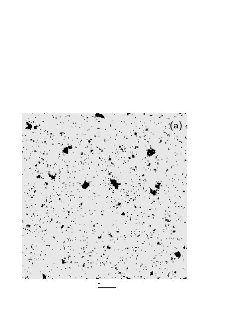
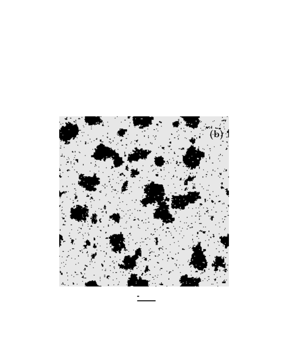
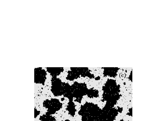
FIG. 1.: Snapshots showing the time evolution of the system configuration during a typical Monte Carlo (MC) simulation for $L$=250, $T$=0.8$T_{\rm c}$, and $|H|$=0.15, for which the lifetime $\tau\approx 392$ MCSS. Light gray represents the metastable spin direction and black the stable spin direction. While supercritical droplets in one snapshot can also be identified in the next, the subcritical fluctuations are uncorrelated between snapshots. The two characteristic lengths, $R_{0}\!\approx\!25$ and $R_{c}\!\approx\!2.5$, are shown by the long and short bar below each snapshot, respectively. (a) $t=80$ MCSS. A few supercritical droplets are seen, but most of the black pixels represent subcritical fluctuations. (b) $t=260$ MCSS. Many large supercritical droplets are growing against the metastable background. (c) $t=390$ MCSS$\approx\tau$. The magnetization is close to zero, several of the supercritical droplets have coalesced, and the stable phase is close to percolating. Microscopic equilibrium fluctuations appear as light specks inside the stable-phase regions. Figure courtesy of G. Korniss.

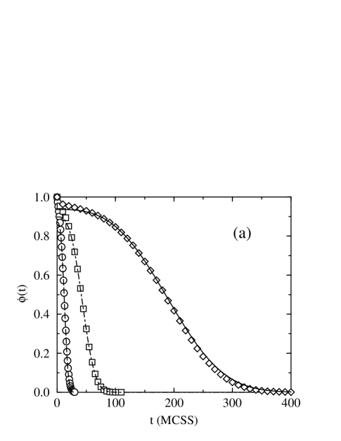
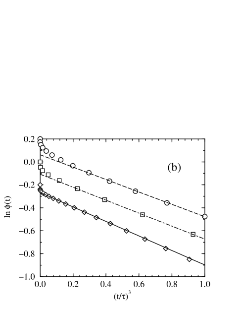
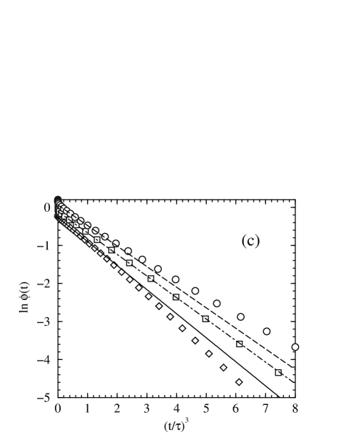
FIG. 2.: MC (points) and fitted KJMA results (lines) for the relaxation function of the Ising model, $\phi(t)$, for $L$=256 and $T$=0.8$T_{\rm c}$. Results are shown for $|H|$=0.2 ($\Diamond$ and solid curve) and 0.4 ($\Box$ and dot-dashed curve), both in the MD regime, and for $|H|$=0.8 ($\circ$ and dashed curve), slightly beyond the mean-field spinodal. The lifetimes are $\tau\approx 186$ MCSS for $|H|$=0.2, $\tau\approx 41$ MCSS for $|H|$=0.4, and $\tau\approx 12$ MCSS for $|H|$=0.8. (a) Linear scale vs $t$. Derivatives of data such as these provide estimates for transient currents in ferroelectric switching[26] and electrochemical potential-step experiments.[42, 43] (b) Semi-logarithmic scale vs $(t/\tau)^{3}$. For clarity, the data for $|H|$=0.8 and 0.2 have been displaced by $\pm 0.2$, respectively. (c) Same as (b), but plotted for $t/\tau\leq 2$ to show the expected deviations of the MC data from the KJMA approximation for later times.

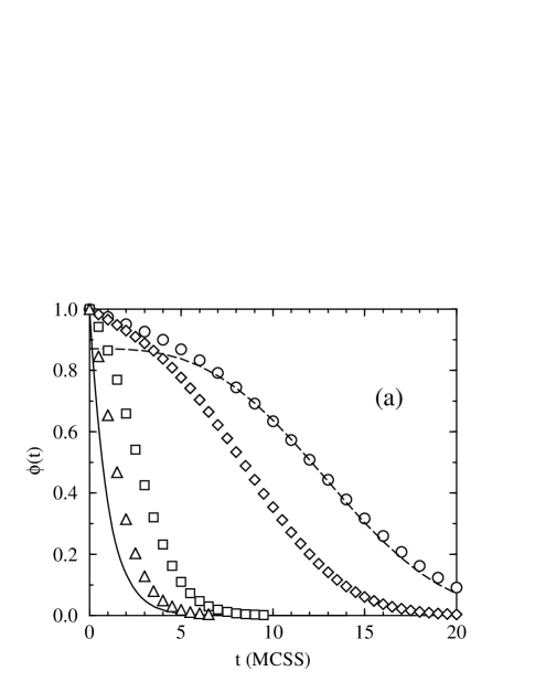
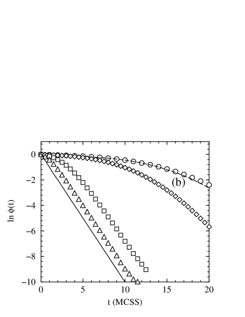
FIG. 3.: MC results for $\phi(t)$ in the strong-field regime at $|H|$=0.8 ($\circ$ and dashed curve, repeated from Fig. 2 for comparison), 1.0 ($\Diamond$), 2.0 ($\Box$), and 3.0 ($\triangle$). The lifetimes are $\tau\approx 8.42$ MCSS for $|H|$=1.0, $\tau\approx 2.70$ MCSS for $|H|$=2.0, and $\tau\approx 1.42$ MCSS for $|H|$=3.0. The solid curves represent exponential relaxation, which is the exact result in the limit $|H|\rightarrow\infty$. (a) Linear scale. (b) $\ln\phi(t)$ vs $t$, emphasizing the approach towards exponential decay with increasing $|H|$.

FIG. 4.: Stable magnetization, $m_{\rm s}$ ($\Diamond$), and metastable magnetization, $m_{\rm ms}$ ($\circ$ and $\Box$), shown vs $H$. The data points for $m_{\rm ms}$ represented as $\circ$ are based on the selection criterion (a) in Sec. IV A, and those represented as $\Box$ on criterion (b). The data are for $L\!=\!256$ except for $H\!=\!-0.15$ and $-$0.12, which correspond to $L\!=\!1024$. The thin solid curves are transfer-matrix (TM) results. For $H\!>\!0$ the curve represents the equilibrium magnetization as obtained for an $N\!\times\!\infty$ system with $N\!=\!9$, which is seen to be in complete agreement with the MC results. For $-0.2\!<\!H\!<\!0$ the curve represents the metastable magnetization corresponding to “the first lobe” [see Appendix B] for $N\!=\!9$, while the solid circles represent the maximum of this lobe for $N\!=\!5$, …, 9 from left to right. For $H\!<\!-0.2$ the curves and solid circles represent “the second lobe” for $N\!=\!5$, …, 9 from left to right.

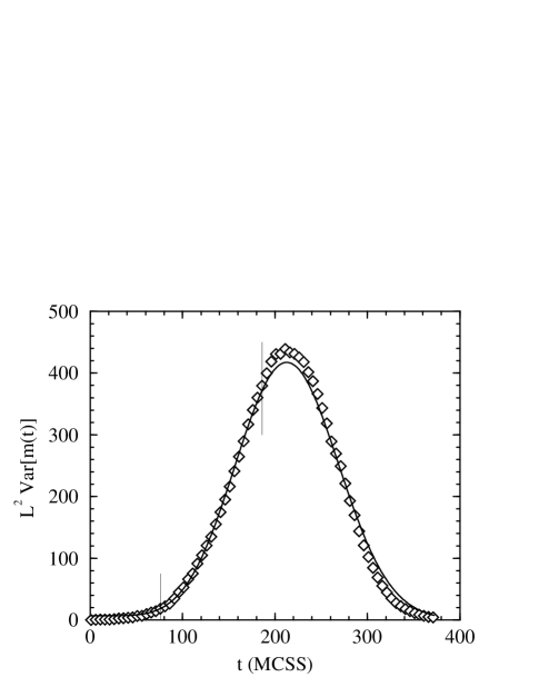
FIG. 5.: An example of $L^{2}$Var[$m(t)$] as obtained from a comparison of 100 independent MC simulations ($\Diamond$) and from a least-squares fit of the KJMA theoretical expression, Eq. (50), (solid curve). This particular result corresponds to $|H|$=0.2. The thin vertical lines mark the time interval $[t_{\rm min},\tau]$, over which the fitting was performed.

FIG. 6.: The average radial growth velocity of the domains of stable phase, $v(T,|H|)$, vs $|H|$. The circles and squares (corresponding to the same selection criteria as in Fig. 4) are the velocities obtained by fitting Eq. (50) to the MC results for $\mbox{Var}[m(t)]$. The diamonds are the velocities obtained in MC simulations of a growing plane interface in which nucleation inside the single-phase domains is suppressed – a “tame” interface. The thin dashed curve and the solid curve represent the analytical linear-response and nonlinear-response approximations for the “tame” interface velocities,[65] Eq. (C2).

FIG. 7.: The nucleation rate $I(T,|H|)$, computed using Eq. (54) with values of $b(|H|)$ and $v(|H|)$ obtained from fits to $\phi(t)$ and Var$[m(t)]$, respectively. The dashed curve is a one-parameter fit to the exact asymptotic result, Eq. (17).

FIG. 8.: MC and KJMA results for the correlation function $G(r,\tau(|H|))$ for $|H|$=0.2 ($\Diamond$, solid curve), $|H|$=0.4 ($\Box$, dot-dashed curve), and $|H|=0.8$ ($\circ$, dashed curve).

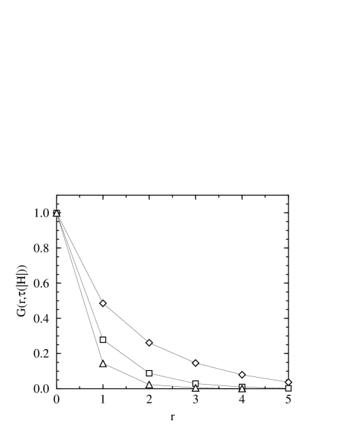
FIG. 9.: MC results for the correlation function $G(r,\tau(|H|))$ in the strong-field regime for $|H|$=1.0 ($\Diamond$), $|H|$=2.0 ($\Box$), and $|H|$=3.0 ($\triangle$). The lines connecting the data points are merely guides to the eye. Note the very short ranges of these correlation functions.

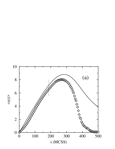
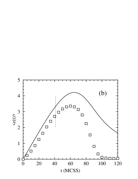
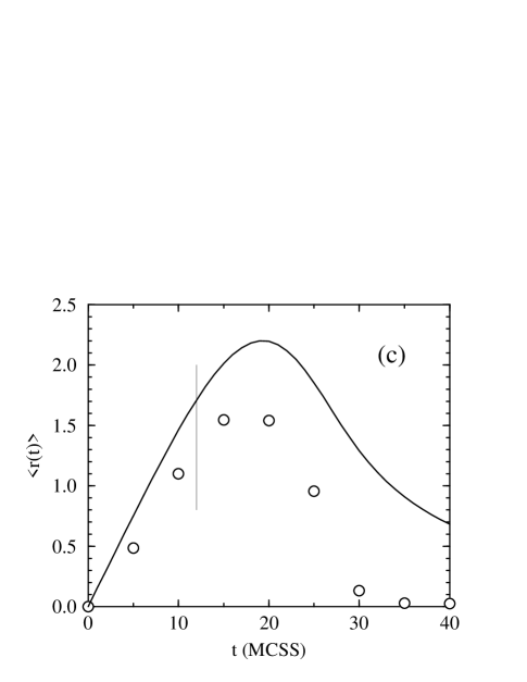
FIG. 10.: MC and KJMA results for the first moment of $G(r,t)$, $\langle r(t)\rangle$. Note the reasonable agreement at early and intermediate times. The rapid decrease of the MC characteristic length at late times reflects the acceleration of the decay of the metastable phase due to interface-tension effects during the droplet-coalescence regime. In each panel the thin vertical line marks $\tau(|H|)$. (a) $|H|$=0.2. (b) $|H|$=0.4. (c) $|H|$=0.8.

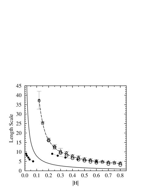
FIG. 11.: Field dependence of the characteristic lengths: the critical droplet diameter $2R_{c}$ (solid curve), the mean separation between droplets of stable phase $R_{0}$ ($\Diamond$, $\bigtriangleup$, and dashed curve) and twice the maximum of $\langle r(t)\rangle$, $2r_{\rm max}$ ($\circ$). Two sets of estimates for $R_{0}$ are shown: A$v/(Iv^{2})^{1/3}$ ($\Diamond$ with error bars) and $v\tau$ ($\bigtriangleup$ and dashed curve). The lengths that characterize the mesoscopic structure, $R_{0}$ and $r_{\rm max}$, remain proportional over the whole range of fields studied. The two chains of solid circles relate the strip widths $N$ of the transfer-matrices used to calculate $m_{\rm ms}$ (Sec. IV A and Appendix B) to the values of $H$ for which $m_{\rm ms}$ so calculated has a maximum. The data points correspond to those shown by the same symbols in Fig. 4. The chain between $H\!=\!0$ and 0.1 represents the first lobe, and the chain between $H\!=\!0.2$ and 0.6 represents the second lobe; in both cases $N\!=\!9$, $...$, 5 from left to right. Comparison of $N$ to the characteristic lengths indicate that the first lobe samples only subcritical fluctuations, while the second lobe also samples rare supercritical fluctuations in the constrained ensemble represented by the TM eigenspaces.

FIG. 12.: Two-parameter scaling plot of the normalized correlation function $G\left(r,\tau(|H|)\right)/G_{\rm KJMA}\left(0,\tau(|H|)\right)$. The data points are MC results and the solid curve is the scaling form of the KJMA correlation function $\Gamma(r,t)$, Eq. (55). The MC results are shown for $|H|$=0.2 and $t$=185 MCSS ($\Diamond$), and for $|H|$=0.25 and $t$=110 MCSS ($\Box$). These fields and times are chosen such that ${r_{0}}/R_{0}$$\approx$0.97 in both cases.

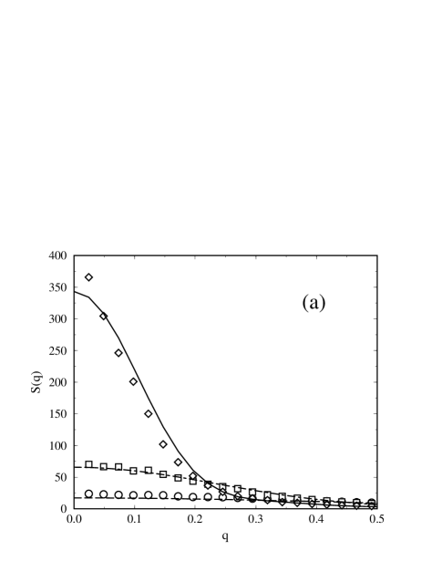
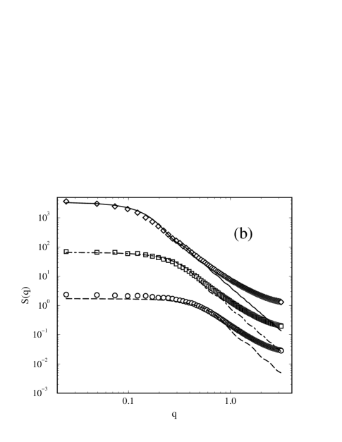
FIG. 13.: The structure factor $S\left(q,\tau(|H|)\right)$. The data points correspond to MC results and the curves to theoretical results calculated by taking the Fourier transform of the KJMA results for $G(r,t)$. Results are shown for $|H|$=0.2 ($\Diamond$, solid curve), $|H|$=0.4 ($\Box$, dotdashed curve), and $|H|$=0.8 ($\circ$, dashed curve). (a) Linear scale. (b) Log-log scale. For clarity, the results for $|H|$=0.2 and 0.8 have been offset by $\pm$ two decades, respectively.

FIG. 14.: The nineteen largest transfer-matrix eigenvalues $\lambda_{\alpha}$, plotted vs $H$ as $-(T/N)\ln|\lambda_{\alpha}|$ for $N\!=\!6$. The lowest-lying branch (dot-dashed line), which corresponds to the dominant eigenvalue $\lambda_{0}$, is the equilibrium free energy per spin. The metastable branch is represented by the heavy curve segments. The solid circles represent the points along each segment, where the magnetization $m_{\alpha}(T,H)$ has its extremum. These points correspond to those similarly marked in Figs. 4 and 11.

REFERENCES

-
[1]
Permanent address:
University of Puerto Rico, Mayaguez, PR 00681.
Electronic address: raf ramos@rumac.upr.clu.edu. - [2] Permanent address: Florida State University, Tallahassee, FL, 32306-4130. Electronic address: rikvold@scri.fsu.edu. URL: http://www.scri.fsu.edu/rikvold.
-
[3]
Electronic address:
novotny@scri.fsu.edu.
URL: http://www.scri.fsu.edu/novotny. - [4] A. N. Kolmogorov, Bull. Acad. Sci. USSR, Phys. Ser. 1, 355 (1937).
- [5] W. A. Johnson and P. A. Mehl, Trans. Am. Inst. Mining and Metallurgical Engineers 135, 416 (1939).
- [6] M. Avrami, J. Chem. Phys. 7, 1103 (1939); 8, 212 (1940); 9, 177 (1941).
- [7] U. R. Evans, Trans. Faraday Soc. 41, 365 (1945).
- [8] By October, 1998, The Institute of Scientific Information (ISI) Science Citation Index database lists over 2100 journal citations to the first article in Ref. [6]. This number does not include citations in books.
- [9] F. P. Price and W. J. H. J. Phys. Chem. 75, 2839 (1971).
- [10] C. P. Yang and J. F. Nagle, Phys. Rev. A 37, 3993 (1988); W. W. Vanosdol, Q. Ye, M. L. Johnson, and R. L. Biltonen, Biophysical J. 63, 1011 (1992).
- [11] K. Jouppila, J. Kansikas, and Y. H. Roos, J. Dairy Sci. 80, 3152 (1997); C. J. Kedward, W. Macnaughtan, J. M. V. Blanshard, and J. R. Mitchell, J. Food Science 63, 192 (1998).
- [12] T. Huang, T. Tsuji, M. R. Kamal, and A. D. Rey, Phys. Rev. B 58, 789 (1998).
- [13] M. Hort, B. D. Marsh, and T. Spohn, Contributions to Mineralogy and Petrology 114, 425 (1993).
- [14] K. R. Elder, F. Drolet, J. M. Kosterlitz, and M. Grant, Phys. Rev. Lett. 72, 677 (1994).
- [15] Y. Yamada, N. Hamaya, J. D. Axe, and M. Shapiro, Phys. Rev. Lett. 53, 1665 (1984).
- [16] J. D. Axe and Y. Yamada, Phys. Rev. B 34, 1599 (1986).
- [17] H. Hermann, N. Mattern, S. Roth, and P. Uebele, Phys. Rev. B 56, 13888 (1997).
- [18] J. M. Rickman, W. S. Tong, and K. Barmak, Acta Materialia 45, 1153 (1997).
- [19] H.-J. Jou and M. T. Lusk, Phys. Rev. B 55, 8114 (1997).
- [20] Y. Ishibashi and Y. Takagi, J. Phys. Soc. Jpn. 31, 506 (1971).
- [21] P. Chandra, Phys. Rev. A 39, 3672 (1989).
- [22] H. M. Duiker and P. D. Beale, Phys. Rev. B 41, 490 (1990).
- [23] P. D. Beale, Integrated Ferroelectrics 4, 107 (1994).
- [24] H. Orihara and Y. Ishibashi, J. Phys. Soc. Jpn. 61, 1919 (1992).
- [25] H. Orihara, S. Hashimoto, and Y. Ishibashi, J. Phys. Soc. Jpn. 63, 1031 (1994); S. Hashimoto, H. Orihara, and Y. Ishibashi, J. Phys. Soc. Jpn. 63, 1601 (1994).
- [26] L. Mitoseriu, V. Tura, and A. Stancu, Phys. Lett. A 196, 272 (1994).
- [27] D. Ricinschi et al., J. Phys.: Condens. Matter 10, 477 (1998).
- [28] V. Shur, E. Rumyantsev, and S. Makarov, J. Appl. Phys. 84, 445 (1998).
- [29] A. A. Hirsch and G. Galeczki, J. Magn. Magn. Mater. 114, 179 (1992).
- [30] H. L. Richards, S. W. Sides, M. A. Novotny, and P. A. Rikvold, J. Magn. Magn. Mater. 150, 37 (1995).
- [31] H. L. Richards, M. A. Novotny, and P. A. Rikvold, Phys. Rev. B 54, 4113 (1996).
- [32] H. L. Richards et al., Phys. Rev. B 55, 11521 (1997).
- [33] P. A. Rikvold, M. A. Novotny, M. Kolesik, and H. L. Richards, in Dynamical Phenomena in Unconventional Magnetic Systems, edited by A. T. Skjeltorp and D. Sherrington (Kluwer, Dordrecht, 1998), p. 307.
- [34] X. Kou, M. A. Novotny, and P. A. Rikvold, submitted to IEEE Trans. Magn.
- [35] S.-B. Choe and S.-C. Shin, J. Appl. Phys. 81, 5743 (1997); Appl. Phys. Lett. 70, 3612 (1997); Phys. Rev. B 57, 1085 (1998); J. Appl. Phys. 83, 6952 91998).
- [36] E. Bosco and S. K. Rangarajan, J. Chem. Soc., Faraday Trans. 1 77, 1673 (1981); B. Bhattacharjee and S. K. Rangarajan, J. Electroanal. Chem. 302, 207 (1991); E. Bosco, J. Chem. Phys. 97, 1542 (1992).
- [37] M. H. Hölzle, U. Retter, and D. M. Kolb, J. Electroanal. Chem. 371, 101 (1994).
- [38] M. S. Maestre et al., J. Electroanal. Chem. 373, 31 (1994).
- [39] C. Saravanan, P. Sunthar, and E. Bosco, J. Electroanal. Chem. 375, 59 (1994).
- [40] T. Dretschkow and T. Wandlowski, Ber. Bunsenges. Phys. Chem. 101, 749 (1997).
- [41] T. Fukuda and A. Aramata, J. Electroanal. Chem. 440, 153 (1997).
- [42] P. A. Rikvold, A. Wieckowski, and R. A. Ramos, in Electrochemical Materials Synthesis and Modification, Mat. Res. Soc. Symp. Proc. Ser., Vol. 451, edited by P. C. Andricacos et al. (Materials Research Society, Pittsburgh, 1997), p. 61.
- [43] P. A. Rikvold, G. Brown, M. A. Novotny, and A. Wieckowski, Colloids and Surfaces A 134, 3 (1998).
- [44] N. Fanelli, S. Zalis, and L. Pospisil, Microchem. J. 59, 9 (1998).
- [45] A. C. Finnefrock, et al., Phys. Rev. Lett. 81, 3459 (1998).
- [46] O. M. Becker, J. Chem. Phys. 96, 5488 (1992).
- [47] B. D. Marsh, J. Petrology 39, 553 (1998); R. Morishita, Mathematical Geology 30, 409 (1998).
- [48] M. Karttunen, N. Provatas, T. Ala-Nissilä, and M. Grant, J. Stat. Phys. 90, 1401 (1998).
- [49] K. Sekimoto, Phys. Lett. A 105, 390 (1984); J. Phys. Soc. Jpn. 53, 2545 (1984); Physica 135A, 328 (1986); Int. J. Mod. Phys. B 5, 1843 (1991).
- [50] S. Ohta, T. Ohta, and K. Kawasaki, Physica 140A, 478 (1987).
- [51] S. W. Sides, R. A. Ramos, P. A. Rikvold, and M. A. Novotny, J. Appl. Phys. 79, 6482 (1996); J. Appl. Phys. 81, 5597 (1997).
- [52] S. W. Sides, P. A. Rikvold, and M. A. Novotny, J. Appl. Phys. 83, 6494 (1998); Phys. Rev. Lett. 81, 834 (1998); Preprint cond-mat/9809136, Submitted to Phys. Rev. E.
- [53] V. Garrido and D. Crespo, Phys. Rev. E 56, 2781 (1997).
- [54] H. J. Meyer, R. Lacmann, and H. Zimmermann, J. Crystal Growth 135, 571 (1994).
- [55] V. Sessa, M. Fanfoni, and M. Tomellini, Phys. Rev. B 54, 836 (1996).
- [56] V. A. Shneidman, K. A. Jackson, and K. M. Beatty, Phys. Rev. B, in press.
- [57] P. A. Rikvold and B. M. Gorman, in Annual Reviews of Computational Physics I, edited by D. Stauffer (World Scientific, Singapore, 1994), p. 149, and references cited therein.
- [58] C. M. Newman and L. S. Schulman, J. Math. Phys. 18, 23 (1977).
- [59] R. J. McCraw and L. S. Schulman, J. Stat. Phys. 18, 293 (1978).
- [60] V. Privman and L. S. Schulman, J. Phys. A 15, L231 (1982); J. Stat. Phys. 31, 205 (1982).
- [61] C. C. A. Günther, P. A. Rikvold, and M. A. Novotny, Phys. Rev. Lett. 71, 3898 (1993).
- [62] C. C. A. Günther, P. A. Rikvold, and M. A. Novotny, Physica A 212, 194 (1994).
- [63] J. S. Langer, Ann. Phys. (N.Y.) 41, 108 (1967); Phys. Rev. Lett. 21, 973 (1968); Ann. Phys. (N.Y.) 54, 258 (1969).
- [64] N. J. Günther, D. A. Nicole, and D. J. Wallace, J. Phys. A 13, 1755 (1980).
- [65] P. A. Rikvold and M. Kolesik, in preparation.
- [66] D. M. Townsley, M. A. Novotny, M. Kolesik, and P. A. Rikvold, in preparation.
- [67] E. N. M. Cirillo and J. L. Lebowitz, J. Stat. Phys. 90, 211 (1998).
- [68] L. Onsager, Phys. Rev. 65, 117 (1944).
- [69] C. N. Yang, Phys. Rev. 85, 808 (1952).
- [70] C. N. Yang and T. D. Lee, Phys. Rev. 87, 404 (1952), ; 87, 410 (1952). The term “lattice gas” was apparently first used and its equivalence to the Ising model first discussed in these two papers.[71].
- [71] R. K. Pathria, Statistical Mechanics, Second Edition (Butterworth-Heinemann, Oxford, 1996).
- [72] R. J. Glauber, J. Math. Phys. 4, 294 (1963).
- [73] K. Binder and D. W. Heermann, Monte Carlo Simulation in Statistical Physics. An Introduction. Third Edition. (Springer, Berlin, 1997).
- [74] N. Metropolis et al., J. Chem. Phys. 21, 1087 (1953).
- [75] G. Brown, P. A. Rikvold, M. A. Novotny, and A. Wieckowski, J. Electrochem. Soc., in press.
- [76] G. Brown, P. A. Rikvold, S. J. Mitchell, and M. A. Novotny, in Interfacial Electrochemistry: Theory, Experiment, and Applications, edited by A. Wieckowski (Marcel Dekker, New York, 1999).
- [77] K. Binder, Phys. Rev. B 8, 3423 (1973).
- [78] P. A. Rikvold, H. Tomita, S. Miyashita, and S. W. Sides, Phys. Rev. E 49, 5080 (1994).
- [79] W. H. Press, S. A. Teukolsky, W. T. Vetterling, and B. P. Flannery, Numerical Recipes in C, Second Edition (Cambridge U. Press, Cambridge, 1992).
- [80] J. D. Gunton, M. San Miguel, and P. S. Sahni, in Phase Transitions and Critical Phenomena, Vol. 8, edited by C. Domb and J. L. Lebowitz (Academic, New York, 1983).
- [81] J. Lee, M. A. Novotny, and P. A. Rikvold, Phys. Rev. E 52, 356 (1995).
- [82] C. K. Harris, J. Phys. A 17, L143 (1984).
- [83] C. Rottman and M. Wortis, Phys. Rev. B 24, 6274 (1981).
- [84] R. K. P. Zia and J. E. Avron, Phys. Rev. B 25, 2042 (1982).
- [85] H. Tomita and S. Miyashita, Phys. Rev. B 46, 8886 (1992).
- [86] Y. C. Chiew and E. D. Glandt, J. Colloid Interface Sci. 99, 86 (1984); P. A. Rikvold and G. Stell, J. Colloid Interface Sci. 108, 158 (1985). These two papers discuss a generalization of Eq. (28) to volume fractions and specific interface areas in models of random two-phase materials and porous media.
- [87] C. D. Van Siclen, Phys. Rev. B 54, 11845 (1996); M. Tomellini and M. Fanfoni, Phys. Rev. B 55, 14071 (1997).
- [88] G. Yu and J. K. L. Lai, J. Appl. Phys. 79, 3504 (1996); G. Yu, Phil. Mag. Lett. 75, 43 (1997); G. Yu, S. T. Lee, J. K. L. Lai, and L. Ngai, J. Appl. Phys. 81, 89 (1997); G. Yu, Y. K. L. Lai, and W. Zhang, J. Appl. Phys. 82, 4270 (1997).
- [89] M. C. Weinberg, D. P. Birnie, and V. A. Shneidman, J. Non-Crystalline Solids 219, 89 (1997).
- [90] V. A. Shneidman and M. C. Weinberg, Ceramic Trans. 30, 225 (1993); J. Noncryst. Solids 160, 89 (1993).
- [91] A. Milchev, K. Binder, and D. W. Heermann, Z. Phys. B 63, 521 (1986).
- [92] Starting with systems fully magnetized parallel to the field, we sampled every 50 MCSS in runs of 10,000 MCSS, after first allowing 2000 MCSS for equilibration. Statistical errors were calculated in the standard way from the variance in each run.
- [93] Expression coined by K. Sekimoto, private communication.
- [94] P. Devillard and H. Spohn, Europhys. Lett. 17, 113 (1991).
- [95] This method is also used in Ref. [56].
- [96] M. Kardar, G. Parisi, and Y.-C. Zhang, Phys. Rev. Lett. 58, 2087 (1986).
- [97] B. Grossmann, H. Guo, and M. Grant, Phys. Rev. A 43, 1727 (1991).
- [98] I. M. Lifshitz, Zh. Éksp. Teor. Fiz. 42, 1354 (1962) [Sov. Phys. JETP 15, 939 (1962)].
- [99] S. M. Allen and J. W. Cahn, Acta Metall. 27, 1085 (1979).
- [100] W. H. Press, S. A. Teukolsky, W. T. Vetterling, and B. P. Flannery, Numerical Recipes in Fortran, Second Edition (Cambridge U. Press, Cambridge, 1992).
- [101] W. K. Burton, N. Cabrera, and F. C. Frank, Phil. Trans. Roy. Soc. (London) Ser. A 243, 299 (1951).
- [102] J. E. Avron, H. van Beijeren, L. S. Schulman, and R. K. P. Zia, J. Phys. A 15, L81 (1982).
- [103] R. A. Ramos, P. A. Rikvold, and M. A. Novotny, in Physical Phenomena at High Magnetic Fields II, edited by Z. Fisk, L. Gor’kov, D. Meltzer, and R. Schrieffer (World Scientific, Singapore, 1996), p. 380.
- [104] A. Guinier and G. Fournet, Small-Angle Scattering of X-rays (Wiley, New York, 1955).
- [105] C. Domb, Adv. Phys. 9, 149 (1960).
- [106] A. B. Bortz, M. H. Kalos, and J. L. Lebowitz, J. Comput. Phys. 17, 10 (1975).