[

Generalized Dielectric Breakdown Model

Abstract

We propose a generalized version of the Dielectric Breakdown Model (DBM) for generic breakdown processes. It interpolates between the standard DBM and its analog with quenched disorder, as a temperature like parameter is varied. The physics of other well known fractal growth phenomena as Invasion Percolation and the Eden model are also recovered for some particular parameter values. The competition between different growing mechanisms leads to new non-trivial effects and allows us to better describe real growth phenomena. Detailed numerical and theoretical analysis are performed to study the interplay between the elementary mechanisms. In particular, we observe a continuously changing fractal dimension as temperature is varied, and report an evidence of a novel phase transition at zero temperature in absence of an external driving field; the temperature acts as a relevant parameter for the “self-organized” invasion percolation fixed point. This permits us to obtain new insight into the connections between self-organization and standard phase transitions.

]

Fractal growth phenomena, such as viscous fingering, electric discharges in dielectrics, fracture propagation and fluid flow in porous media, have attracted much attention in recent years. In the study of these phenomena many models – the Diffusion Limited Aggregation (DLA) [1], Dielectric Breakdown Model (DBM) [2], and Invasion Percolation (IP)[3] to quote only but a few – have been introduced as a first step towards the understanding of the dynamic emergence of fractal structures in nature. These models have been quite successful in reproducing the essence of the above complex phenomena by capturing some key ingredients. Their simplicity has also allowed for analytical studies of the scale invariant properties of corresponding structures [4, 5].

To proceed further in this field there are two possible directions: One is to identify possible interrelations between these models and understand their eventual universality or fundamental differences. For example, these irreversible processes have a much lower degree of universality than their counterparts in equilibrium statistical mechanics, but still the basic “dynamical screening” mechanisms leading to fractal growth (as opposed to the growth of compact clusters) can be categorized in some generic classes, among them that arising from the external physical field (e.g. a Laplacian field in the DBM), or extremal dynamics and memory effects [4, 6]. The second is to make these models more realistic or closer to real phenomena. For example, the interplay between these different mechanisms has been hardly studied so far. For instance, it has been recently found that the combination of Laplacian screening and extremal dynamics, results in a much stronger screening effect than that of each single mechanism, leading to fractal dimensions lower than those characterizing the two different elementary mechanisms [7].

Here we present a step forward in both of the previous directions. On one hand, we introduce a generalization of the available models in a broader class which permits us the identification of relevant parameters in more realistic growth phenomena.

FIG. 1.: Schematic diagram showing the limiting cases of our model as a function of temperature and the parameter $\eta$.

On the other hand this broader class is theoretically important as it is able to cast in a coherent framework apparently unrelated physical situations. This gives a new perspective that permits us to clarify the roles of the single physical mechanisms in competition, namely external driving fields, quenched disorder, and thermal noise. The relative strengths of these effects are modulated in our model by three parameters, $\eta$, $a$ and $T$ respectively. For some particular values of these parameters different well known growth models are recovered (see figure 1). For $T=0$ we have QDBM, in the infinite $T$ limit the model reduces to the DBM; at $\eta=0$ and zero temperature we have IP, while for generic temperatures we have compact (EDEN [8]) growth with a temperature dependent correlation length.

Let us now present the model, that we name as Generalized Dielectric Breakdown Model (GDBM). The medium in which a breakdown process propagates is discretized as a regular (say hypercubic) lattice. The relevant degrees of freedom are placed on the bonds connecting lattice sites. Each of these bonds can either be broken or not. Unbroken bonds are characterized by a given variable, $s_{i}$, that can take different values (for instance, this can represent in a sketchy way the elongation of a spring at $i$). The simplest situation one can think of is that of $s_{i}$ being a spin-like variable $s_{i}=\pm 1$. We consider a cylindrical geometry with lateral periodic boundary conditions. This geometry, in fact, avoids all complications due to the discretized nature of the lattice, (like the anisotropy of growth along the diagonals of the lattice, relevant in geometries with radial symmetry [5]). We are interested in studying the process by which the bonds in the interface break down successively, and in how the cluster of broken bonds evolves.

The dynamics proceeds as follows. First of all we assume that the breakdown process is quasi-static, i.e. only one bond is broken at each time step, and it is in the interface of previously unbroken bonds, this is, the cluster of broken bonds is connected. As initial condition we take as broken all the bonds in the lower row of the cylinder. Secondly, there are two distinct processes going on during the breakdown, the time scales of which are widely separated. The first, slow process, is the dynamics of breakdown itself. The second, fast process, is the relaxation of the field configuration and of variables $s_{i}$ after a breakdown event. In between two consecutives breakings the bond variables relax to their associated equilibrium state, whose associated energy or Hamiltonian will be defined later. The separation of time-scales is a common ingredient in many models for fractal growth and self-organized criticality [9], and is physically a quite reasonable assumption.

We now define the fast dynamics in between two consecutive breakdowns. Every bond $i$ is subject to a stress Laplacian field $E_{i}$. As in the DBM this (electric) field is given by the solution of the Laplace equation with the appropriate boundary conditions on the growing fracture [2, 5], namely the potential is $1$ at the upper border of the cylinder (upper electrode) and $0$ on the lower one and on the broken bonds. This field acts over the bonds modulated by a parameter $\eta$ [2], $E_{i}^{\eta}$, for $\eta=0$ any dependency on the external field is canceled.

The second physical ingredient is quenched disorder. At each bond we define a random resistance $x_{i}$, distributed as $\pi(x)=ax^{a-1}$, $x\in[0,1]$ and $a\in[0,\infty)$. This gives an idea of the bond tolerance to applied stresses; the larger $x_{i}$ the larger the resistance. Other probability distributions can be used without affecting the properties of the model. We now define an effective local field accounting for the electric field and the disorder $h_{i}=E_{i}^{\eta}/x_{i}$ which acts on the local degree of freedom $s_{i}$ generating an interaction energy given by

$$H_{i}=h_{i}s_{i}.$$ (1)

There are looser bonds, with $x_{i}$ large, which can accommodate a larger stress $E_{i}^{\eta}$ induced by the Laplacian field, and tighter, or more fragile, bonds, with $x_{i}$ small.

In general one could also include nearest neighbor interactions, so that $H_{i}=h_{i}s_{i}+\sum_{j}Js_{i}s_{j}$ to account for material rigidity. However, for the situations we are interested in, the local stress fields are much larger than the coupling $J$ and $J$ can be neglected.

The equilibrium statistical mechanics of each bond variable among two successive breakdown processes is easily determined by introducing the temperature $T$. The partition function factorizes on the bonds: $Z(\{h_{i}\},T)=\prod_{i}z(h_{i},T)$ and

$\displaystyle z(h_{i},T)=\sum_{s_{i}=\pm 1}e^{-h_{i}s_{i}/T}=2\cosh(h_{i}/T).$

We can now calculate, as a function of $h_{i}$ and $T$, all averages. In particular

$\displaystyle\langle{s_{i}}\rangle=-T\frac{\partial}{\partial h_{i}}\ln z(h_{i},T)=\tanh(h_{i}/T)$

$\displaystyle\langle{\delta s_{i}^{2}}\rangle=1-\tanh^{2}(h_{i}/T)$

are of interest. It is clear that $\langle{s_{i}}\rangle$ is a measure of the stress exerted by the external field on the bond $i$ and $\langle{\delta s_{i}^{2}}\rangle$ measures the strength of thermal fluctuations.

We consider the breaking probability $P_{i}$ of a bond as an increasing function of the stress, and as a decreasing function of the amplitude of its thermal fluctuations; it is indeed when the local degree of freedom is thermally frozen in a stressed state, i.e. when it is very rigid, that breakdown is more likely to occur. On the other hand when the variance is large, the spin can better absorb stress and is more flexible.

Guided by these considerations, the simplest dimensionless expression for the breaking probability $P_{i}$ is

$$P_{i}\propto\frac{\langle{s_{i}}\rangle}{\sqrt{\langle{\delta s_{i}^{2}}\rangle}}=\sinh(h_{i}/T).$$ (2)

At each time step all the $P_{i}$ are calculated, and with the corresponding probabilities one bond is broken. After that, the boundary conditions are automatically modified and the field $E$ updated at each point. Using the hypothesis of time scale separation, $z(h_{i},T)$ and $P_{i}$ are automatically updated, a new bond breaks down in the interface, and the process is iterated.

The behavior of the model in some limiting cases can be analytically sorted out.

(i) For $T\gg 1$ one can expand Eq. (2) around $h_{i}=0$, and find $P_{i}\propto E_{i}^{\eta}/x_{i}$. In this limit the disorder does not play a relevant role and one obtains back the DBM (this same fact was already observed in [10]).

(ii) For $T\ll 1$, on the other hand, the argument of the $\sinh$ is very large and essentially only the bond with the largest $h_{i}$ has a finite probability to break as $T\to 0$. In this way an extremal dynamics is generated, namely the quenched version of the DBM [10, 11].

(iii) By setting $\eta=0$, the dependence on the physical field is canceled and we have a purely geometrical process. In fact, in that limit we obtain the IP extremal dynamics. For $T>0$ a characteristic length is generated in the dynamics as we will show later by performing numerical simulations, and one observes asymptotically compact clusters, i.e. EDEN [8] growth.

It is worth to stress that the previous limiting cases are quite general. For example one could also consider continuous degrees of freedom $\sigma_{i}$ taking values on a range $[-x_{i},x_{i}]$. The specific equations change but the limiting form of $P_{i}$ given by Eq. (2) for $T\gg 1$ and $T\ll 1$, remains unchanged.

In order to study the properties of our model in more detail in generic cases, we have performed numerical simulations. Each bond of the lattice is assigned a growth probability as in Eq. 2 and the dynamics starts from the lowest electrode, which represents the seed of the growth process. As soon as the fracture pattern reaches the upper limit of the lattice, the dynamics is stopped, and a new realization starts. We performed a set of about $50$ realizations of the dynamics of size $L\times 4L$ with $L\!=\!64,128$, for a wide range of values of the temperature $T$, and different values of $\eta$ and $a$. For each set of realizations we compute by using a box-counting method [12] the fractal dimension, $D_{f}$, of the resulting clusters. Data are collected only in the central $L\times 2L$ part of the lattice, which is sufficiently far from the lower transient regime and the upper interfacial region [5]. In Fig. 2a-b we show a plot of $D_{f}(T)$ vs. $T$ for $L\!=\!64$ and $L\!=\!128$ respectively and different values of $a$ and $\eta$, while in Tab. I we give some numerical values of $D_{f}(T)$ (for $\eta\!=\!1,a\!=\!1$). caca

$T$	$0.1$	$0.5$	$1.0$	$5.0$	$500.0$
$D_{f}(T)[L=64]$	$1.15(2)$	$1.32(3)$	$1.41(3)$	$1.56(3)$	$1.63(4)$
$D_{f}(T)[L=128]$	$1.14(2)$	$1.32(1)$	$1.44(2)$	$1.59(2)$	$1.65(2)$

TABLE I.: Fractal dimension of aggregates of size $L=64,128$ for different values of $T$ ($a=1,\eta=1$).

It can be verified that, as predicted, in the limits $T\to 0$ and $T\to\infty$ the model approaches the QDBM and DBM known values of $D_{f}$, $1.15$ and $1.66$ respectively [2, 10, 7, 5]. The transition from the QDBM-like behavior to the DBM-like one is smooth and continuous (Fig. 2), with continuously varying $D_{f}(T)$.

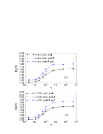
FIG. 2.: a) fractal dimension $D_{f}(T)$ of GDBM vs. the parameter $T$ (dimensionless) for system size $L=64$ (a) and $L=128$ (b) with different values of $\eta,a$. Note the irrelevance of $a$ (disorder) for high temperatures.

We have checked that the critical properties of the model become less and less sensible to the value of $a$ as the temperature $T$ is raised (see Fig. 2), in agreement with our previous arguments. In our picture of the breakdown phenomena, this means that for very high temperatures, the thermal disorder is more relevant that the quenched one.

When the Laplacian field is removed ($\eta=0$) the properties of the model change dramatically. We observe a transition from an IP-like behavior to an EDEN like behavior. For a value of $T=0.02$ (the smallest value that we are able to implement in simulations), we get already compact growth, with $D_{f}=1.98\pm 0.02$ for size $L=128$; observe that the slight deviation from $D_{f}=2$ being a finite size effect) (see Fig. 3)

FIG. 3.: Results of the box-counting analysis for a very small temperature $T=0.02$ and $\eta=0$. The values $D_{f}=1.97(2)$ for $L=64$ and $D_{f}=1.98(2)$ for $L=128$ we get correspond to asymptotically compact clusters and, are very far from the IP fractal dimension $D_{f}\sim 1.89$.

This result is not affected by changes of the disorder strength. In fact, it can be easily shown that the extremal dynamics we recover in the $T=0$ limit, is independent on the value of $a$ if there is no Laplacian field [7, 4].

To analyze in more detail the crossover from IP to EDEN model we studied the correlation properties of the clusters in the following way. A fractal structure is characterized by the presence of voids of all sizes with no characteristic length; that is precisely the situation for $T=0$ in our model. However, for $T>0$ voids are still present in the clusters but they have a characteristic, temperature dependent, size $s_{c}(T)$. Since voids are compact objects, the square root of $s_{c}(T)$ represents the correlation length $\xi(T)$ of our model. We have studied the void distribution of our model for different small $T$ and system size $L=128$. By collapse plot techniques we have obtained the behavior of $s_{c}(T)=\xi^{2}(T)$ shown in Fig. 4, and we have found a power law divergence of the correlation length as we approach $T=0$, with an associated anomalous exponent $\nu=1.07(6)$. This power law divergence of the correlation length can be interpreted as the hallmark of a second order phase transition along the temperature axis, with $T_{c}=0$. This is in line with recent results found for other self-organized models [9]. To test this hypothesis we studied the avalanche distribution $D(s)$ for different $T$’s (for a definition of avalanches see for example [4]). This distribution is fitted by the scaling function: $D(s)=s^{-\tau}f(s/s_{0})$ where $s$ is the avalanche size, $\tau$ is the avalanche exponent, $f(x)$ goes to a constant for $x\to 0$ and falls exponentially for $x\to\infty$, and $s_{0}$ is the cutoff size of the avalanches away from the critical point. By assuming $s_{0}\sim T^{-\frac{1}{\sigma}}\sim\xi^{D_{f}}$, and $\langle s\rangle\sim T^{-\gamma}$, where $\langle{s}\rangle=\sum_{1}^{\infty}sD(s)$, we obtain the usual scaling relations among avalanche exponents $\frac{1}{\sigma}=\nu D_{f}\,,\,\gamma=\frac{(2-\tau)}{\sigma}$. Our simulations give (Fig.4): $1/\sigma=1.69(5)$, $\gamma=0.72(5)$, $\tau=1.60(2)$, $D_{f}=1.87(3)$. These values together with the above estimation of $\nu$ are in good agreement with the scaling relations among exponents, and support the interpretation of the transition at $T=0$ from IP to EDEN model as a second order dynamical phase transition (a more detailed report on numerical as well as analytical results will be given in a forthcoming paper.

In summary, we have presented a general model which include DBM, QDBM, IP and EDEN models as limiting cases, and permits to interpolate among them by describing the the interplay between quenched disorder, thermal disorder and external stress fields. This represents a step towards an unification of the models actually used to describe fractal growth phenomena, under a common picture. We report a continuous change in the fractal dimension as temperature is risen interpolating from QDBM to DBM, and a novel phase transition from the extremal (self-organized) IP fixed point to EDEN type of growth. This can trace a connection between fractal growth dynamics and ordinary critical phenomena.

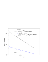
FIG. 4.: (a): $\log_{10}$-$\log_{10}$ plot of $s_{c}(T)=\xi^{2}(T)$ versus $T$ for the GDBM model without field. We find $\xi(T)\sim T^{-\nu}$ with $\nu=1.07(6)$. We interpret this as an evidence of a second order phase transition at $T_{c}=0$. (b): Scaling of $s_{0}$ and $\langle{s}\rangle$ vs. $T$.

ACKNOLEDGMENTS This work has been partially supported by TMR Network, contract number FMRXCT980183, and TMR grant ERBFMBICT960925 to M.A.M.

REFERENCES

- [1] T. A. Witten and L. M. Sander, Phys. Rev. Lett. 47, 1400 (1981).
- [2] L. Niemeyer, L. Pietronero and H. J. Wiessmann, Phys. Rev. Lett. 52,1033 (1984).
- [3] D. Wilkinson and J. F. Willemsen, J. Phys. A 16, 3365 (1983).
- [4] R. Cafiero, A. Gabrielli, M. Marsili and L. Pietronero, Phys. Rev. E 54, 1406 (1996); M. Marsili and M. Vendruscolo, Europhys. Lett. 37, 505 (1997).
- [5] A. Erzan, L. Pietronero and A. Vespignani, Rev. Mod. Phys. 67, 3 (1995).
- [6] M. Marsili, G. Caldarelli, and M. Vendruscolo, Phys. Rev. E 53, R1 (1996).
- [7] R. Cafiero, A. Gabrielli, M. Marsili, L. Pietronero and L. Torosantucci, Phys. Rev. Lett. 79, 1503 (1997).
- [8] M.Eden, 4th Berkeley Symp. on Mathematical Stat. and Prob., pag.223 (1961).
- [9] G.Grinstein, in Scale Invariance, Interfaces and Nonequilibrium Dynamics, Vol.344 of NATO ASI, series B, ed.s A.McKane et al. (Plenum, New York, 1995). A. Vespignani, R. Dickman, M. A. Muñoz, and S. Zapperi, Pre-print 1998.
- [10] F. Family, Y. C. Zhang and T. Vicsek, J. Phys. A 19, L733 (1986).
- [11] L. De Arcangelis, A. Hansen, H. J. Herrmann and S. Roux, Phys. Rev. B 40, 877 (1989).
- [12] K. J. Falconer, Fractal Geometry: Mathematical Foundation and Application J. Willey and sons, New York, 1990.