Zero temperature phase transitions in spin-ladders: phase diagram and dynamical studies of $\rm\bf Cu_{2}(C_{5}H_{12}N_{2})_{2}Cl_{4}$

Abstract

In a magnetic field, spin-ladders undergo two zero-temperature phase transitions at the critical fields $H_{c1}$ and $H_{c2}$. An experimental review of static and dynamical properties of spin-ladders close to these critical points is presented. The scaling functions, universal to all quantum critical points in one-dimension, are extracted from (a) the thermodynamic quantities (magnetization) and (b) the dynamical functions (NMR relaxation). A simple mapping of strongly coupled spin ladders in a magnetic field on the exactly solvable XXZ model enables to make detailed fits and gives an overall understanding of a broad class of quantum magnets in their gapless phase (between $H_{c1}$ and $H_{c2}$). In this phase, the low temperature divergence of the NMR relaxation demonstrates its Luttinger liquid nature as well as the novel quantum critical regime at higher temperature. The general behavior close these quantum critical points can be tied to known models of quantum magnetism.

1 Introduction

It is well known that long-range order is destroyed by quantum fluctuations in one-dimensional antiferromagnets. If the importance of quantum effects is ubiquitous in one-dimension, a wide variety of ground states can nevertheless be found in nature. Some systems have a continuum of low energy modes, some have an energy gap above a unique ground state, other dimerize. Where do these differences come from? In simple terms, the role of quantum effects is simply to ”connect” different classical ground states (for example the Néel states $|\uparrow,\downarrow,\uparrow,\downarrow,\ldots\rangle$ and $|\downarrow,\uparrow,\downarrow,\uparrow,\ldots\rangle$) by tunneling processes. Depending of the strength of the tunneling matrix elements, which can usually be measured by a coupling constant $g$, the system will be more or less localized around a classical ground states. As $g$ is varied, the system can delocalize at a critical value $g_{c}$. When the system delocalizes in spin space, the ground state becomes a rotationally invariant singlet and in all the cases which will be considered here, an energy gap $\Delta$ appears simultaneously in the energy spectrum. Many physical aspects determine the strength of quantum fluctuations. The integer or half-integer nature of the spin considered modify drastically selections rules for quantum-processesHaldane83 . This is why integer-spin chains for which $g$ exceed $g_{c}$ have an energy gap, while half-integer spin-chains remain gapless ($g\leq g_{c}$). Other physical parameters (exchange constants, applied magnetic fields) also enter in the precise determination of the coupling strength $g$. Systems for which the coupling constant can be continuously varied by an experimentally controllable parameter, such as a magnetic field, are rare. In this paper we review a few 1-D antiferromagnets where such zero temperature critical points have been observed, with a particular emphasis on $\rm Cu_{2}(C_{5}H_{12}N_{2})_{2}Cl_{4}$ (also known as CuHpCl)Chaboussant97a ; Chaboussant97b ; Chaboussant98 , a spin-ladder compound, where a complete set of experiments exist.

At a quantum critical point Hertz76 ; Chubukov94 ; Sachdev94 ; Sachdev97 ; Sondhi97 , the system switches from one ground state into another. Specifically when $g\leq g_{c}$, antiferromagnetic correlation functions decay as power laws and the system is nearly ordered. When $g$ is increased above $g_{c}$, a gap opens up and the range of antiferromagnetic correlation become finite, of the order of $\xi_{g}\simeq a/|g-g_{c}|$ ($a$ is the lattice constant). In the vicinity of $g_{c}$, one has to go to relatively long lengthscale, exceeding $\xi_{g}$ to be able to tell in which phase the system is. In other words, the nature of the ground state is manifest only at long lengthscale. At finite temperature spin-flip processes become possible. They cut spin-correlations off at a lengthscale $\xi_{T}$ which can be estimated in the quantum-disordered phase ($g\geq g_{c}$) as the mean distance between excitations. Since their energies are higher than the energy gap $\Delta\simeq 1/|g-g_{c}|$ above the ground state, their density is activated. Hence when $\mbox{$k_{\rm B}$}T<\Delta$, the mean distance between excitations $\xi_{T}$ greatly exceed $\xi_{g}$ and thermal fluctuations are not really relevant. On the other hand, when $\mbox{$k_{\rm B}$}T\geq\Delta$, their density is governed by the relative value of $\mbox{$k_{\rm B}$}T-\Delta$ compared to the bandwidth of the triplet excitations. When $\Delta$ is small compared to $\mbox{$k_{\rm B}$}T$ and this bandwidth, $\xi_{g}$ exceeds very rapidly $\xi_{T}$. In this case, the density of excitations are determined by $\mbox{$k_{\rm B}$}T$ alone which become the only relevant energy scale. In this limit, dynamical properties are similar to those of a simple paramagnet ($1/T_{1}\rightarrow cst$) while thermodynamics quantities remain nontrivial. This regime is (improperly) named the quantum critical regime, because most properties are determined by the single lengthscale $\xi_{T}$ as in ordinary phase transitions.

Figure 1: Phase diagram of spin-ladders in a magnetic field. The magnetic field (vertical axis), can be thought as a tuning parameter for the quantum coupling constant $g$. Below $H_{c1}\Leftrightarrow g_{c}$, the coupling constant $g$ exceeds $g_{c}$ ($H\leq H_{c1}\Leftrightarrow g\geq g_{c}$). This phase has a singlet ground state and an energy gap. Above $H_{c1}$, the coupling constant $g$ drops below $g_{c}$: the phase is magnetic and gapless and belongs to the same universality class as the Heisenberg XXZ model. The dotted lines represent the crossover lines where $\xi_{g}\simeq\xi_{T}$ separating two quantum regimes just described (where $\xi_{g}$ is the relevant quantum correlation length) from the quantum critical regime dominated by $\xi_{T}$. For the system discussed in this paper the quantum critical behavior at the upper critical field $H_{c2}$ is similar and will be discussed in the next sections. The shaded area between critical fields is a 3D ordered phase stabilized by transverse interactions (see Sec. 5).

To summarize, there are two-relevant lengthscales at a quantum critical point, the quantum correlation length $\xi_{g}$ and the thermal length $\xi_{T}$. Depending on their relative values, different regimes exists. They are represented graphically in Fig. 1, on the H-T phase diagram appropriate to spin-ladders. The regions dominated by quantum effects are (a) the gapped spin-liquid phase below line A, (b) the XXZ or Luttinger liquid phase to the left of line C and (c) the gapped polarized phase above line B. The quantum critical region is found to the right of these crossover line and extends down to $T=0$ at the critical fields $H_{c1}$ and $H_{c2}$. Each regime will clearly be identified using thermodynamic and $1/T_{1}$ NMR relaxation measurements which allow to place precisely the crossover lines on this phase diagram.

The differents sections are organized as follows: a brief description of several families of gapped antiferromagnets having an H-T phase diagram similar to the one shown in Fig. 1 can be found in Sec. 2. A description of the structure and the interactions relevant to CuHpCl, the 1D ladder system chosen for our case study, is given in Sec. 3. A mapping of strongly coupled ladder in a magnetic field onto the XXZ Heisenberg model is introduced in Sec. 4. It is used throughout the rest of the paper to fit and interpret experimental data. In Sec. 5, the different phases shown in Fig. 1 are identified using high-field magnetization data. The XXZ model is used to fit the low temperature data and to give a physical model for the ordered phase observed between $H_{c1}$ and $H_{c2}$. Section 6 is devoted to the dynamical processes entering in the NMR relaxation. The different regimes decribed in Fig. 1 are presented in Sec. 7 through $T_{1}^{-1}$ measurements across the entire phase diagram. The Luttinger liquid behavior between $H_{c1}$ and $H_{c2}$ is clearly seen for the first time and compared to the XXZ models. Finally the first scaling analysis for a 1D quantum critical point is presented in Sec. 8 and the paper concludes with some new perspectives.

2 Gapped 1-D antiferromagnets: a broad universality class

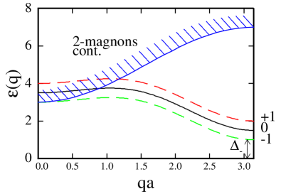
Figure 2: The lowest lying excitations form a triplet branch, split by the Zeeman field, or other anisotropic forces. They are separated from a unique singlet ground state by energy gaps $\Delta_{+},\Delta_{0},\Delta_{-}$. In absence of anisotropies, they are split by the Zeeman energy, $\Delta_{\pm}=\Delta_{0}\pm g\mu_{B}H$. The shape of the dispersion relation across the Brillouin zone depends on the exchange interactions specific to each 1-D system. In particular, the energy gap may be at $qa=\pi$ (S=1 chains, ladders) or at $q=0$ (dimerized chains with sufficiently large antiferromagnetic second-neighbor exchange). Similarly, a two-”magnons” continuum may intersect the triplet branch and have a lower energy in some region of the Brillouin zone. In this universality class, there are no singlet states in the gap.

There are three known families of quasi 1-D materials belonging to the same universality class, with an H-T phase diagram similar to Fig. 1. They can all be described by the same quantum-field theory, the O(3) non-linear $\sigma$-modelHaldane83 ; Affleck89 ; Levy97 in a magnetic field. Their excitation spectrumUhrig96 in a weak magnetic field is represented in Fig. 2. The lower critical field $H_{c1}$, is reached when the lowest energy gap $\Delta_{-}$ vanishes. The upper critical field $H_{c2}$ is usually reached when the highest energy state of the $\epsilon_{-}(q)$ branch is below the singlet energy. An approximate representation of their singlet ground-states are represented in Fig. 3.

The know families of 1-D antiferromagnets in this universality class are:
- (i) Quasi 1D-antiferromagnetic compounds with two alternating exchange constants $J_{1}$ and $J_{2}$ have been known for over two decades to have a gap (top of Fig. 3). For spin-1/2 alternating chains, the spectrum is identical to Fig. 2 and in the strong coupling limit ($J_{1}\gg J_{2}$), the energy gap is $\Delta\approx J_{1}-\frac{J_{2}}{2}-\frac{3}{8}\frac{J_{2}^{2}}{J_{1}}$. Very nice thermodynamic studiesDiederix79 of $Cu(NO_{3})_{2}.2.5H_{2}0$ have identified the existence of two critical fields $H_{c1}\approx J_{1}-J_{2}/2\simeq 2.8$ T and $H_{c2}\equiv 2J_{1}\simeq 4.5$ T. In spite of the modest value of $H_{c1}$ and $H_{c2}$, dynamical properties close to these critical points have never been thoroughly mapped out neither by NMR relaxation measurements nor by neutron scattering. Considering the interest in quantum phase-transition, this interesting compound should be revisited.
- (ii) Spin-1 Heisenberg antiferromagnetic chainsHaldane83 with a sufficiently weak planar anisotropy have in zero magnetic field a triplet excitation branch separated by an energy gap $\Delta\approx 0.41\times J$ from the unique singlet ground state. The most thoroughly studied compound in this family is NENPRenard87 . Because of the presence of a planar anisotropy, this system has three different lower critical fields (9.8, 13.3 and 14 Tesla)Ajiro89 ; Katsumata89 depending on the orientation of the field with respect to the anisotropy axes. The upper critical field which has not been measured should exceed 86 Tesla. Thermodynamic and dynamical measurementsFujiwara93 have been carried out at the lower critical field and provide very valuable insight on zero-temperature phase transitions.
- (iii) Spin-ladders are quasi-1D structures where a finite number of antiferromagnetic chains are coupled by a transverse antiferromagnetic exchange. Ladders with an odd-number of coupled chains are gapless and belong to the same universality class as the spin-1/2 Heisenberg chain Dagotto96 . On the other hand, spin-1/2 ladders with an even number of legs are gapped and form a singlet ground-state with short ranged spin correlations (spin-liquid). While several compounds with ladder-like magnetic structure exist Azuma94 ; Hiroi95 , the only system where the quantum critical point $H_{c1}$ is experimentally accessible is CuHpCl, a coordination compound made up by stacking binuclear molecules in a ladder structureChiari90 . ThermodynamicChaboussant97a ; Hammar98 and dynamic quantitiesChaboussant97b ; Chaboussant98 have been measured over the entire phase diagram and give a relatively complete experimental picture of a zero-temperature phase transition.

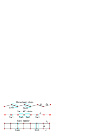
Figure 3: Three families of gapped antiferromagnets. Top, dimerized chains: the antiferromagnetic bond $J_{1}$ dominates $J_{2}$. Singlet valence bonds are preferentially localized on these bonds. Middle, integer spin chains. The ground state can also be viewed as a product of valence bondsAffleck87 , by decomposing each spin 1 in two spin-1/2 and forming valence bonds with the pair of spin-1/2 at the extremity of each bonds (valence bond solid). Bottom: spin ladders. In the strong coupling limit ($J_{\perp}\gg J_{\parallel}$), singlet bonds are localized on the rungs of the ladder.

We now describe its structure, and the relevant magnetic interactions in this material.

3 CuHpCl, a 1-D spin ladder in the strong coupling limit

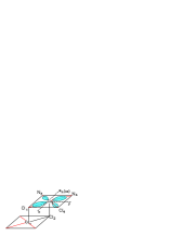
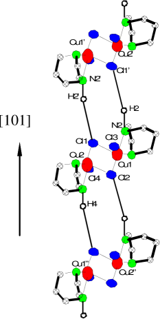
Figure 4: Top: Representation of the parallel plane geometry of the $Cu^{++}$ orbitals. Bottom: stacking of the molecular units in a ladder structure along the $[101]$ axis.

The molecular unit is a binuclear structure with two $Cu^{++}$ ions (spin 1/2) each lying in a middle of two parallel distorted square-structuresChiari90 . At the vertices of each square, one finds two chlorine and two nitrogen ions as depicted in the top of Fig. 4. There are two super-exchange paths through the chlorine ions $Cl_{1}$ and $Cl_{2}$ bridging the copper ions. However, the $p_{z}$ orbitals of the chlorine ions are nearly orthogonal to the $Cu^{++}$ $d_{xy}$ orbital. The resulting exchange constant between the copper ions $J_{\perp}\approx 13.5\>K$, is found to be weaker than in other materials with similar $Cu-Cu$ distance. The organic rings, on the outside of the ionic-core just described, contribute further to the delocalization of the unpaired $Cu^{++}$ orbital. Each molecular unit stacks up in the [101] direction of this $P2_{1}/c$ molecular crystal (see Fig. 4). In addition to the van-der-Vaals forces, the organic rings allow a weak hydrogen bonding between molecules, along which a super-exchange path can propagate. In spite of the relatively large intermolecular $Cu-Cu$ distance, the orbital overlaps are favorable and lead to an intermolecular-exchange interaction $J_{\parallel}\approx 2.45\>K$ along the ladder. Strictly speaking, due to the low symmetry, there are small differences in $Cu-Cu$ distances along the ladder above and below each molecular unit. Because the bridging entities have the same symmetries, these small differences are not expected to modulate significantly the exchange ($J_{\parallel}$) along the legs. The translational invariance is nevertheless naturally broken, making any additional lattice (spin-Peierls) instabilities less favorable. Comparison of thermodynamic properties to numerical simulationsHawyard96 have demonstrated that the other possible magnetic cross-bondings between the legs are weak and need not be considered. On the other hand, it is now clear that there is also a weak inter-ladder super-exchange, probably also mediated by a weak hydrogen bonding between organic rings. If it is not relevant in the gapped phases, it induces at low-T a 3D-ordered phase in the gapless region between $H_{c1}$ and $H_{c2}$Hammar98 . While this phase has been observed in specific heat measurements, its actual structure has not been determined experimentally.

4 Hamiltonian representations of strongly-coupled spin-ladders

For most purposes, it will be sufficient to consider a quasi-1D ladder Hamiltonian in a magnetic field ${\mathcal{H}}={\mathcal{H}}_{1}+{\mathcal{H}}_{2}+{\mathcal{H}}_{Z}$, where

$${\mathcal{H}}_{1} = J_{\perp}\sum_{i=1}^{N}{\vec{S}}_{2i-1}\cdot{\vec{S}}_{2i}$$ (1)

$${\mathcal{H}}_{2} = J_{\parallel}\sum_{i=1}^{2N}{\vec{S}}_{i}\cdot{\vec{S}}_{i+2},$$ (2)

(even spins are on one leg and odd spins are on the other). The weak $g$-factor anisotropy ($g_{\perp}\approx 2.03,g_{\parallel}\approx 2.11$) observed in EPR measurementsChaboussant97a may be retained in the Zeeman Hamiltonian, ${\mathcal{H}}_{Z}=\sum_{i=1,\alpha}^{2N}g_{\alpha}\mu_{B}S_{i}^{\alpha}H_{\alpha}$. In the strong coupling limit ($J_{\perp}\gg J_{\parallel}$), it is possible to give a straightforward description of the low-energy states in a magnetic field, treating ${\mathcal{H}}_{2}$ as a perturbationTotsuka98 ; Mila98 . The eigenstates of ${\mathcal{H}}_{1}+{\mathcal{H}}_{Z}$ which describes isolated dimers in a magnetic field, are built from the singlet (valence bonding) and triplets $\makebox[5.0pt]{ \put(0.0,-2.0){\line(0,1){3.0}} \put(0.0,4.0){\line(0,1){3.0}} \put(0.0,-2.0){\circle*{2.5}} \put(0.0,7.0){\circle*{2.5}}}_{+1}$, $\makebox[5.0pt]{ \put(0.0,-2.0){\line(0,1){3.0}} \put(0.0,4.0){\line(0,1){3.0}} \put(0.0,-2.0){\circle*{2.5}} \put(0.0,7.0){\circle*{2.5}}}_{0}$, $\makebox[5.0pt]{ \put(0.0,-2.0){\line(0,1){3.0}} \put(0.0,4.0){\line(0,1){3.0}} \put(0.0,-2.0){\circle*{2.5}} \put(0.0,7.0){\circle*{2.5}}}_{-1}$ (antibonding) on each rung. Since we are interested in the critical region, where the Zeeman energy is of the order of $J_{\perp}$, it is legitimate to project ${\mathcal{H}}_{2}$ on the restricted Hilbert space generated by the lowest dimers states, and $\makebox[5.0pt]{ \put(0.0,-2.0){\line(0,1){3.0}} \put(0.0,4.0){\line(0,1){3.0}} \put(0.0,-2.0){\circle*{2.5}} \put(0.0,7.0){\circle*{2.5}}}_{-1}$. The matrix elements of ${\mathcal{H}}_{2}$ between neighboring dimers can be represented on this subspace by a $2\times 2$ matrix, which is expressed in second-quantized notation as

$${\mathcal{H}}_{2}^{\rm eff}=\frac{J_{\parallel}}{2}\sum_{r=1}^{N}\left(t^{\dagger}_{r}t_{r+1}+t_{r}t^{\dagger}_{r+1}+n_{r}n_{r+1}\right).$$ (3)

The fermionic operator $t^{\dagger}$ creates the triplet state $\makebox[5.0pt]{ \put(0.0,-2.0){\line(0,1){3.0}} \put(0.0,4.0){\line(0,1){3.0}} \put(0.0,-2.0){\circle*{2.5}} \put(0.0,7.0){\circle*{2.5}}}_{-1}$ on bond $r\equiv[2i,2i+1]$ (only one triplet per bond is allowed), while $t$ destroys a triplet, leaving a singlet on bond r. The operator $n_{r}\equiv{t^{\dagger}}_{r}t_{r}$ counts the triplet occupation of bond r. In the fermion language, the first two terms represent the kinetic energy while the last term is a short range repulsion between fermions. Since $S^{2}$ and $S_{z}$ are good quantum numbers (${\vec{S}}$ is the total spin), it is convenient to divide the Hilbert space into sectors with a given value of $S_{z}$. In the restricted Hilbert space, each sector specifies the total fermionic occupation since

$$S_{z}=\sum_{r}n_{r}.$$ (4)

The singlet sector is not coupled by ${\mathcal{H}}_{2}^{\rm eff}$ and the singlet eigenstate remains the dimer product $|S=0\rangle=|\makebox[5.0pt]{ \put(0.0,-2.0){\line(0,1){9.0}} \put(0.0,-2.0){\circle*{2.5}} \put(0.0,7.0){\circle*{2.5}}}\makebox[5.0pt]{ \put(0.0,-2.0){\line(0,1){9.0}} \put(0.0,-2.0){\circle*{2.5}} \put(0.0,7.0){\circle*{2.5}}}\ldots\rangle$ with energy $E_{0}=-\frac{3}{4}NJ_{\perp}$. This ground state energy may be compared to a serie expansion in $J_{\parallel}/J_{\perp}$Reigrotzki94 . For the parameters appropriate to CuHpCl, the corresponding singlet energy is only 1.6% lower than in the previous estimate. The reduction of ${\mathcal{H}_{2}}$ to Eq. 3 is therefore appropriate to CuHpCl, at least for qualitative answers.

In the $S=1$ (1-fermion) sector, the Hamiltonian ${\mathcal{H}}_{2}^{\rm eff}$ can also be diagonalized in Fourier space, since the interaction term $n_{r}n_{r+1}$ does not contribute. The dispersion relation of this triplet state is,

$$E_{S_{z}=-1}(q) = J_{\perp}-g_{z}\mu_{B}H+J_{\parallel}\cos(qa),$$ (7)

$$|1,q\rangle = \sum_{r}\exp(iqr)|\makebox[5.0pt]{ \put(0.0,-2.0){\line(0,1){9.0}} \put(0.0,-2.0){\circle*{2.5}} \put(0.0,7.0){\circle*{2.5}}}\ldots\makebox[5.0pt]{ \put(0.0,-2.0){\line(0,1){9.0}} \put(0.0,-2.0){\circle*{2.5}} \put(0.0,7.0){\circle*{2.5}}}_{r-1}\makebox[5.0pt]{ \put(0.0,-2.0){\line(0,1){3.0}} \put(0.0,4.0){\line(0,1){3.0}} \put(0.0,-2.0){\circle*{2.5}} \put(0.0,7.0){\circle*{2.5}}}_{r}\makebox[5.0pt]{ \put(0.0,-2.0){\line(0,1){9.0}} \put(0.0,-2.0){\circle*{2.5}} \put(0.0,7.0){\circle*{2.5}}}_{r+1}\ldots\rangle.$$ (8)

For fields below $g_{z}\mu_{B}H_{c1}\approx\Delta_{0}=J_{\perp}-J_{\parallel}$, there is an energy gap $\Delta_{-}=\Delta_{0}-g_{z}\mu_{B}H$ between the singlet and the $q=\pi/a$ minimum of the triplet branch, as shown in Fig. 2. For fields above $H_{c1}$ or temperatures above the gap $\Delta_{-}/\mbox{$k_{\rm B}$}$, it is necessary to explore the energy spectrum of ${\mathcal{H}}_{2}$ at finite fermion density. In the low-energy sector of the Hilbert space ($\makebox[5.0pt]{ \put(0.0,-2.0){\line(0,1){9.0}} \put(0.0,-2.0){\circle*{2.5}} \put(0.0,7.0){\circle*{2.5}}},\makebox[5.0pt]{ \put(0.0,-2.0){\line(0,1){3.0}} \put(0.0,4.0){\line(0,1){3.0}} \put(0.0,-2.0){\circle*{2.5}} \put(0.0,7.0){\circle*{2.5}}}_{-1}$), a finite fermion density raises the energy of ${\mathcal{H}}_{1}+H_{z}$ with respect to the ground state by an amount proportional to the triplet (fermion) density

$$\delta E=(J_{\perp}-g_{z}\mu_{B}H)\sum n_{r}.$$ (9)

In other words, $\mu\equiv J_{\perp}-g_{z}\mu_{B}H$ acts as the chemical potential for the triplets.

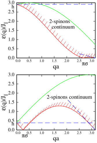
Figure 5: Energy spectrum of transverse excitations in a magnetic field. Top panel: $H\geq H_{c1}$, the incommensurate wavevector is close to the antiferromagnetic point. Lower panel: $H\simeq(H_{c1}+H_{c2})/2$, the incommensurate wave-vector is close the zone center. On both plots, the spin-stiffness $\rho_{s}\propto\sin(\pi-Q_{\sigma})$ is the slope of the bottom edge of the spectrum at $q=\pi$.

The low energy spectrum of ${\mathcal{H}}_{2}^{\rm eff}$ can be described exactly on the restricted Hilbert space: Eq. (3) can be recognized as the fermion representation of the $S=\frac{1}{2}$ XXZ Heisenberg model

$${\mathcal{H}}_{\rm eff} = J_{\parallel}\sum_{i}\left(S_{r}^{x}S_{r+1}^{x}+S_{r}^{y}S_{r+1}^{y}+\frac{1}{2}S_{r}^{z}S_{r+1}^{z}\right)$$ (10)

$$+ H_{\rm eff}\sum_{r}S_{r}^{z}+N\frac{J_{\perp}}{8},$$

in an effective field

$$H_{\rm eff}=J_{\perp}+\frac{J_{\parallel}}{2}-g_{z}\mu_{B}H.$$ (11)

$H_{\rm eff}$ is zero at the midpoint between $H_{c1}=J_{\perp}-J_{\parallel}$ and the upper critical field $H_{c2}\equiv J_{\perp}+2J_{\parallel}$Chaboussant97a . The spin eigenstates of this effective Hamiltonian are a representation of the triplet-singlet subspace ($|\uparrow\rangle\equiv\makebox[5.0pt]{ \put(0.0,-2.0){\line(0,1){3.0}} \put(0.0,4.0){\line(0,1){3.0}} \put(0.0,-2.0){\circle*{2.5}} \put(0.0,7.0){\circle*{2.5}}}_{-1},|\downarrow\rangle\equiv\makebox[5.0pt]{ \put(0.0,-2.0){\line(0,1){9.0}} \put(0.0,-2.0){\circle*{2.5}} \put(0.0,7.0){\circle*{2.5}}}$) on each rung and have nothing to do with the original spin-1/2. In this model, the excitations which carry $\hbar/2$ angular momentum (spinons), have a semionic character, i.e. can only be observed in pairs. In non-zero effective fields ($H_{\rm eff}\neq 0$) the longitudinal and transverse excitations must be distinguished.

Figure 6: The $k=\pi/2$ (a) and $k=\pi$ (c) ground states are superposition of the singlet-triplet configurations shown. The wavevector $k$ refers to the wavevector in the XXZ representation. In ladder representation shown, this wavevector is $k/2$. Excitations are built as Bloch wave of the soliton-antisoliton pairs represented on (b) and (d).

The continuous spectrum of transverse excitations (1-magnon or 2-spinons) is represented on Fig. 5 at two different magnetic fields. At fields just above $H_{c1}$ (Fig. 5, top panel) a new minimum in the spectrum develops at $Q_{\sigma}a=\pi\sigma$, where $\sigma=M(H_{\rm eff})/M_{sat}$ is the spin-polarization of the XXZ-model in an effective field $H_{\rm eff}$. The lower critical field $H\approx H_{c1}$ correspond to the saturation field of the XXZ model, $H_{\rm eff}^{sat}\approx 3J_{\parallel}/2$: the spin-polarization $\sigma$ in $H_{\rm eff}^{\rm sat}$ is $-1$ and the ladder magnetization $m$ is zero. Just above $H_{c1}$, the soft modes at $\pi/a$ and $Q_{\sigma}$ are very close: the spin stiffness $\rho_{s}\propto(1+\sigma)\propto m$ goes to zero and a large low-energy spectral weight exists close to the antiferromagnetic point. The situation is quite different close to $H_{\rm eff}=0$ (i.e. half-way between $H_{c1}$ and $H_{c2}$), where the incommensurate wave-vector $Q_{\sigma}$, is close to the zone center (Fig. 5, lower panel). For longitudinal fluctuations, the incommensurate minima in the two cases considered are essentially interchanged with respect to transverse fluctuations.

It is useful to ”translate” the XXZ incommensurate states just described into the valence bond representation of ladder states. The pictorial images of the incommensurate ground states shown in Fig. 6, close to $J_{\perp}-J_{\parallel}/4$ and $J_{\perp}+J_{\parallel}/2$, are appropriate on short lengthscales (quantum fluctuations destroy the periodicity $Q_{\sigma}$ on long lengthscales). Low energy excitation above the ground state are Bloch waves of the soliton-antisoliton defects depicted on Fig. 6: this builds a coherent superposition $\alpha\makebox[5.0pt]{ \put(0.0,-2.0){\line(0,1){9.0}} \put(0.0,-2.0){\circle*{2.5}} \put(0.0,7.0){\circle*{2.5}}}+\beta\makebox[5.0pt]{ \put(0.0,-2.0){\line(0,1){3.0}} \put(0.0,4.0){\line(0,1){3.0}} \put(0.0,-2.0){\circle*{2.5}} \put(0.0,7.0){\circle*{2.5}}}_{-1}$ (transverse fluctuation) at wavevector $Q_{\sigma}$.

Since so many exact results are known for the XXZ model, the mapping discussed here will prove to be extremely useful in the analysis experimental data. The high field magnetization of CuHpCl clearly establishes the correspondence with the phase diagram show in Fig. 1.

5 Identification of the different phases with high-field magnetization measurements

The weak g-factor anisotropy and the monoclinic symmetry of this crystal, allow a straightforward determination of the magnetization by torque magnetometry: if the field is applied along the ${\hat{z}}$ axis, which does not coincide with the principal axes ${\hat{a}},{\hat{b}},{\hat{c}}$, the magnetization is not collinear with H, and a torque $\tau\propto M\times H$ can be measured. The magnetization curves of a $100\mu g$ monocrystal have been measured with an ultrasensitive AC torque magnetometerCrowell96 ; Chaboussant97a .

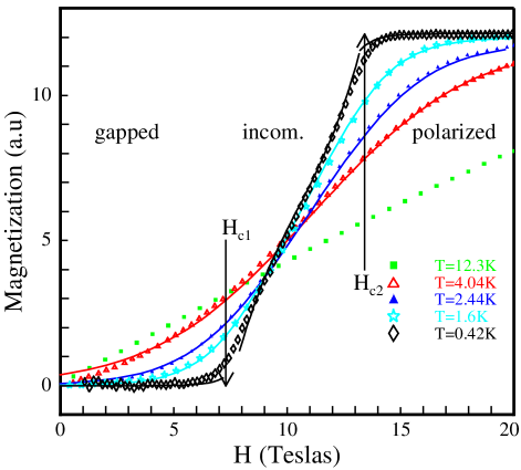
Figure 7: Magnetization of CuHpCl between 0 and 20 T, at different temperatures. The symbols are experimental data points, while the solid lines are the fits to the XXZ model described in the text, using the procedure outlined in appendix B. From the lowest temperature curve, two critical fields $H_{c1}$ and $H_{c2}$ are identified. Below $H_{c1}$, the system is unmagnetizable, i.e. forms a singlet ground state separated from $S\neq 0$ excitations. Above $H_{c2}$, the system is fully polarized. The ”incommensurate phase” is between $H_{c1}$ and $H_{c2}$.

It is straightforward to identify the critical field $H_{c1}$ and $H_{c2}$ from the $T=0.42K$ magnetization curve shown in Fig. 7. Below $H_{c1}$, the magnetization is thermally activated with an effective gap $\Delta_{-}$ (this is shown in Fig. 8). Similarly, above $H_{c2}$, the deviation from the saturated magnetization are activated with an energy gap $g_{z}\mu_{B}(H-H_{c2})$ (see NMR section). In appendix A, the energy spectrum of excitations carrying one unit less angular momentum than the fully polarized state are determined. In a ladder, there are two spins in the unit cell, and hence two spin-wave modes. Since the polarized phase is unstable when the lowest energy of these spin-waves drops below the energy of the polarized state, the upper critical field can be specified exactly

$$g_{z}\mu_{B}H_{c2}=J_{\perp}+2J_{\parallel}.$$ (12)

The observed behavior of the magnetization in the different field regions coincides precisely with the zero temperature phases specified on the y-axis of Fig. 1. Quantitatively, the exchange parameters $J_{\perp}\approx 13.5\>K$, $J_{\parallel}\approx 2.45\>K$ are most accurately determined from the values of $H_{c1}$ and $H_{c2}$. $J_{\perp}$ can be identified independently as the magnetic field at which the NMR relaxation rate is maximum in the high temperature limit (see Sec. 7). These numbers have also been checked against (a) the low and high temperature dependence of the susceptibilityChaboussant97a ; Weihong97 , (b) the gap suppression of the low temperature specific heat and (c) the overall bandwidth ($2J_{\parallel}$) of the triplet branch (H=0)Hammar98 measured by neutron scattering. In a numerical study of the ladder magnetization, the presence of a weak cross-exchange coupling between legs has also been investigatedHawyard96 . The conclusion is that this coupling is weak and if non-zero, ferromagnetic. Considering all the experimental and numerical uncertainties, it seems at present unnecessary to keep any additional exchange coupling in the analysis.

The thermodynamic properties for the XXZ model can be computed exactly by the Bethe AnsatzYang66 ; Takahashi72 and the magnetization curves have been evaluated numerically using the procedure described in Appendix B. At temperature below $J_{\perp}$,hightemp the results (Fig. 7, solid lines) agree very well with the experimental magnetization. Considering that there are no adjustable parameters, the mapping of strongly-coupled spin-ladders onto the XXZ model appears to be excellent. In particular, the quantum critical behavior of ladders at $H_{c1}$ is acurately reproduced by this model, a point which is emphasized further in Sec. 8 by constructing explicitly the scaling plots for the magnetization. In the gapped phase, the XXZ mapping progressively loses its validity at small Zeeman splitting (compared to $\Delta$)hightemp . In this limit, it is instructive to compare the temperature dependent magnetization to the free-fermion model proposed by Troyer et al.Troyer94 ; Chaboussant97a where

$$\frac{M}{M_{sat}}=\frac{2z(\beta)\sinh(\beta g_{z}\mu_{B}H)}{1+[2\cosh\beta g_{z}\mu_{B}H]z(\beta)}$$ (13)

and $z(\beta)\approx\exp(-\beta J_{\perp})I_{0}(\beta J_{\parallel})$ In this model, the statistical weights are adjusted in order to reproduce the full spin entropy at high temperature, but the nearest-neighbor repulsion is ignored. Fig 8 shows that, at high temperature, the experimental magnetization is systematically higher that inferred by the free-fermion model (solid lines). At finite temperature, interactions between fermions increase the value of the chemical potential (which is negative in the gapped phase, $\mu\geq-|\Delta_{-}|$). Hence at higher temperature, the effective gap ($|\mu|$) becomes smaller and a higher fermion density is possible. The role of interactions will be further emphasized with the identification of the NMR relaxation processes: the dominant relaxation channel (staggered process) when $H\rightarrow H_{c1}$ would not be possible without interactions.

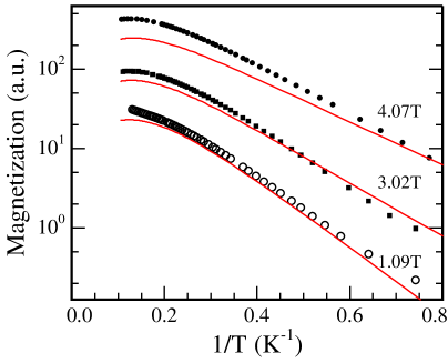
Figure 8: Magnetization of CuHpCl in the gapped phase as a function of $1/T$, at different magnetic fields. The experimental points are compared to the free fermion model of Troyer (solid lines). A systematic deviation from the free-fermion model is observable when their density becomes significant: this emphasize the role of the short range repulsion between fermions.

5.1 Ordered phase

Down to $T=0.1\>K$, magnetization curves show no plateaux nor slope changes which could indicate a 3D ordering transition. The 1D models appear to give a precise account of the magnetization at all temperature. On the other hand, small but sharp peaks in the specific heat have been observed above $H_{c1}$ at low temperatureHammar98 ; Calemzuck98 . After integration of the specific heat at constant field, it is found that the entropy per spin associated to this transition is very small ($<10^{-2}\mbox{$k_{\rm B}$}$/spin). In light of these experimental facts, a second order phase transition appears at low-T between $H_{c1}$ and $H_{c2}$, involving a small change in spin-entropy and no detectable change in magnetization.

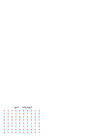
Figure 9: Suggested ordered dimer-state close to half-filling: triplet and singlet bonds form a 3D antiferromagnetic lattice.

When 3D coupling are ignored, the XXZ mapping (Sec. 4) gives a representation in terms of an interacting 1D fluid of spinless fermions (Luttinger liquid). Since there is no magnetization change, the 3D transition takes place at constant fermion density. A very common 3D instability for a 1D Luttinger liquid is a charge density wave ordering. In a valence-bond language, this transition can be viewed as a valence-bond ordering of the 1D $\makebox[5.0pt]{ \put(0.0,-2.0){\line(0,1){3.0}} \put(0.0,4.0){\line(0,1){3.0}} \put(0.0,-2.0){\circle*{2.5}} \put(0.0,7.0){\circle*{2.5}}}_{-1}$ states in a 3D-lattice. This would hardly affect the magnetization which measures the density of $\makebox[5.0pt]{ \put(0.0,-2.0){\line(0,1){3.0}} \put(0.0,4.0){\line(0,1){3.0}} \put(0.0,-2.0){\circle*{2.5}} \put(0.0,7.0){\circle*{2.5}}}_{-1}$ bonds (fermion density) while the quenching of their kinetic energy would be manifest in the specific heat. For a 3D-charge ordering, repulsive interactions between fermions are usually necessary. Antiferromagnetic superexchange between ladders, introduce very naturally an additional repulsion between fermions on different ladders. This antiferromagnetic super-exchange may be represented by,

$${\mathcal{H}}_{inter}=J_{inter}\sum_{\langle k,l\rangle}{\vec{S}}_{k}\cdot{\vec{S}}_{l}$$ (14)

where the sum $\langle k,l\rangle$ is carried over nearest-neighbor spins belonging to different ladders. The physics of a low-T transition should be described by the projection of (14) on the restricted Hilbert space, i.e.

$${\mathcal{H}}_{inter}^{\rm eff}=-\frac{J_{inter}}{4}\sum_{\langle k,l\rangle}\left(t^{\dagger}_{k}t_{l}+t_{k}t^{\dagger}_{l}-n_{k}n_{l}\right),$$ (15)

which has, up to a sign, the same form as ${\mathcal{H}}_{2}^{\rm eff}$. A gauge transformation, switching the phase of hopping operators $t_{2r+1}\rightarrow-t_{2r+1}$ every other rungs, restores an effective antiferromagnetic coupling in the spin model. In the spinless fermion model, a transition to a charge density wave state can only be established close to half filling [$H=(H_{c1}+H_{c2})/2$]Georges98 . It is not known whether this transition persist at low fermion densities. Since this model arise in many context, it will be important to determine its complete phase diagram. Of particular relevance is the commensurate or incommensurate nature of the 3D charge density. The physics of this model is in fact relevant to almost all quasi-1D quantum magnets. For example, in the spin-Peierls compounds $CuGeO_{3}$, there is also a transition to a 3D incomensurate phase, with no change in total magnetization. At the transition, only the local distribution of magnetization changesFagot96 . Eßler and TsvelikEssler97 have shown that the 3D phonon-couplings present in this family of materials can be represented as a transverse exchange between chains in an effective magnetic Hamiltonian. From the point of view of magnetism, this ”charge density wave” ordering cannot be distinguished from a real spin-Peierls transition recently proposed by several authorsCalemzuck98 . It is therefore natural to expect ordered phases with similar structures in all compounds within this universality class.

From the point of view of magnetism, this is an original magnetic state, with a 3D ordered structure of valence bonds. Fig. 9 gives a pictorial representation of this state at half-filling ($(H=H_{c1}+H_{c2})/2$). From this discussion, it is clear that further experimental and theoretical studies of the 3D ordering of strongly coupled ladder are called for.

6 Assigment of NMR lines and identification of the dynamical relaxation processes in the gapped phase

NMR is an ideal tool to probe the low-energy dynamics of quantum magnetsChaboussant97b . When nuclei (here protons) are located at different sites than the electronic spins, the interaction between electronic and nuclear spins are mostly dipolar: the dipolar field ${\vec{h}}_{ij}(t)$ produced by the electronic spin $i$ on the nuclear spin $j$ serves a probe for the dynamical properties. The time-averaged $z$-component $\sum_{i}\langle h^{z}_{ij}\rangle$ of this local field shifts the value of the magnetic field felt by the nucleus by an amount proportional to the local electronic susceptibility $\chi_{i}$

$$K_{j}=\sum_{i}A_{ij}\chi_{i}.$$ (16)

$K_{j}$ depends on the position of the nuclei in the unit-cell through the dipolar sum

$$A_{ij}\propto-\gamma_{e}\gamma_{n}\hbar^{2}\frac{1-3\cos^{2}\theta_{ij}}{|r_{ij}|^{3}}$$ (17)

where $\theta_{ij}$ is the angle between ${\vec{r}}_{ij}$ and $\vec{H}$. $K_{j}$ will be positive if ${\vec{h}}_{j}$ is mostly parallel to H, and negative if its antiparallel. $CuHpCl$ contains 24 protons spins in the unit cell: in the NMR spectrum at $16\>T$ (i.e. in the polarized phase) shown in Fig. 10, there are indeed 24 resolved lines. Their position depends on temperature and follow the T-dependence of the local magnetization. For 16 nuclei the hyperfine shift $K_{j}$ is positive and negative for the 8 remaining. For proton sites which are nearly equivalents, the lines are close together as the local fields (and their fluctuations) are nearly identical. Using the proton positions calculated from X-ray data, it is possible to determine the dipolar sum on each site and assign it to a corresponding line. For example, the outermost line labeled I arise from nuclei $H_{14}\>\&\>H_{23}$ ($A_{I}\approx 2950\>G$) while line II arise from proton $H_{2}$ ($A_{II}\approx-2400\>G$).

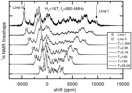
Figure 10: Temperature dependence of the NMR spectrum measured at 16T. The intensities have been normalized to compensate for the gap suppression. Most $T_{1}^{-1}$ measurements have been carried out on Line I and II, which are always located at the extremities of the spectrum for all fields and temperatures. They can be identified with nuclei $H_{14}\>\&\>H_{23}$ (line I) and nuclei $H_{2}$ (line II).

The hyperfine shift is also a measure of the local electronic spin susceptibility $M_{j}/H$. Its temperature dependence is shown in Fig. 11. Below $H_{c1}$ there is, at low temperature, an exponential drop of the hyperfine shift consistent with an activated behavior with a characteristic energy gap $\Delta_{-}$. The dependence observed at $8.7\>T$, just above $H_{c1}$, shows an increase of the local magnetization as the temperature is raised, a very unusual behavior for a magnetic phase (e.g. the magnetization of canted antiferromagnets always decrease with temperature). At low temperature ($\mbox{$k_{\rm B}$}T<J_{\perp}$) it is meaningful to use the XXZ representation, where the system can be viewed as a Luttinger liquid of triplets: in this limit, the presence of a continuum of longitudinal excitation carrying an angular momentum $\hbar$ (see Sec. 4) contributes to an increase of the triplet occupation with temperature. At higher fields, the density of states at small wavevectors gets smaller and a more classical behavior is recovered. In quantitative term, the hyperfine shift observed below $6K\approx J_{\perp}/2$ agrees well with the XXZ mapping and the thermodynamic measurements of $M/H$ (see Fig. 11).

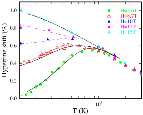
Figure 11: Temperature dependence of the hyperfine shift at different magnetic fields. The thermodynamic measurement of $M/H$ at H=5, 8 and 15T are plotted on the same graph as solid lines. The comparison of the NMR shift to the value of $M/H$ inferred from the XXZ mapping (Sec. 4) at low temperature are drawn as dotted lines. At 8.7 T, in the gapless XXZ-phase, there is first an increase of the local magnetization with temperature, an unusual behavior for a magnetic state.

Temporal fluctuations of the local fields ${\vec{h}}_{ij}(t)$ at the nuclear precession frequency (essentially zero energy) provide the dominant relaxation channel for nuclear spins. The longitudinal spin-lattice relaxation rate of the nucleus i

$$\frac{1}{T_{1}}\bigg{|}_{i} = \int\exp(-i\omega_{n}t)dt\sum_{j}\langle h_{ij}^{+}(t)h_{ij}^{-}(0)\rangle$$

$$= \frac{(\gamma_{n}\gamma_{e}\hbar)^{2}}{2}\sum_{q}\left[F_{\perp}^{i}(q){\mathcal{S}}_{\perp}(q,\omega_{n})\right.$$

$$+ \left.F_{z}^{i}(q){\mathcal{S}}_{z}(q,\omega_{n})\right]$$ (19)

is sensitive to the transverse and longitudinal structure factors

$${\mathcal{S}}_{\perp}(q,\omega_{n}) = \int\exp(-i\omega_{n}t)dt\langle S_{q}^{+}(t)S_{-q}^{-}(0)\rangle,$$ (20)

$${\mathcal{S}}_{z}(q,\omega_{n}) = \int\exp(-i\omega_{n}t)dt\langle S_{q}^{z}(t)S_{-q}^{z}(0)\rangle$$ (21)

through the form factors $F_{z}^{i}$ and $F_{\perp}^{i}$. These quantities are simply the Fourier transform of $|A_{ij}|^{2}$ defined in Eq. 17. They are most easily computed in real space as geometrical dipolar sums: the longitudinal and transverse components of the resultant local field on site i, ${\vec{h}}_{i}=\sum_{j}{\vec{h}}_{ij}$, depend on the actual position of the nucleus i in the unit cell. Depending on the proton site selected, the relative magnitude of the form factors $F_{z}^{i}$ and $F_{\perp}^{i}$ can change by one order of magnitude: this provides a unique way to measure separately all components of the structure factor at $\omega=\omega_{n}$.

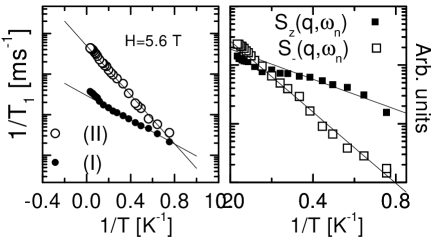
Figure 12: Temperature dependence of the $T_{1}^{-1}$ relaxation rate of sites I and II in the gapped phase ($H=5.6\>T$). At high temperature the relaxation at site II is an order of magnitude faster than at site I, but decreases exponentially at lower temperature with an activation energy $\Delta_{II}\approx 6.8\>K$, twice as large as for site I, $\Delta_{I}\approx 3.4\>K$.

Fig.12 illustrates how different the relaxation on different proton sites can be in the gapped phase ($H=5.6\>T$). If the $T_{1}^{-1}$ behavior of both lines I and II are activated, the activation energy for line II, $\Delta_{II}\approx 6.8\>K$, is twice as large as the activation energy for line I, $\Delta_{I}\approx 3.4\>K$. In a field of $5.6\>T$, the smallest activation energy is $\Delta_{-}=\Delta-g\mu_{B}H\ \approx 3.0\>K$ between the triplet branch $|1,q\rangle$ and the ground state, close to the measured energy $\Delta_{I}$ for line I.

The contribution of one-magnon states $|1,q\rangle$ (cf. Eq. 7) to the structure factor are proportional to $\delta(\omega-E_{1}(q))$: their spectral weight at the nuclear frequency is zero. On the other hand, these states are by no-means exact eigenstates and a number of low-energy scattering processes between magnons can generate a finite spectral weight at low energy. Among them, there are (i) finite matrix elements of ${\mathcal{H}}_{2}$ between triplet states which are ignored in the reduction to the effective Hamiltonian ${\mathcal{H}}_{2}$, (ii) density-density interactions (last term in Eq. 3), which contribute as the square of the density of thermally excited magnons, (iii) other interactions such as interchain couplings and impurity scattering.

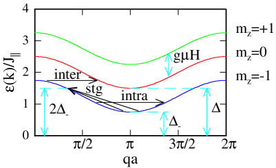
Figure 13: Schematic representation of multi-magnon scattering processes which can drive the NMR relaxation. The intrabranch processes leave $m_{z}$ unchanged and contribute only to ${\mathcal{S}}_{z}$. The interbranch process which involve a spin flip, contribute to ${\mathcal{S}}_{\perp}$ and are quenched one the Zeeman energy ($7.6\>K$ at $5.6\>T$) exceed the triplet bandwidth ($2J_{\parallel}\approx 5\>K$). In the staggered process, two magnons from the bottom of the band $-1$ are scattered into a magnon state at twice the energy: it is governed by the square of the magnon density $n_{-}^{2}\propto\exp(2\Delta_{-})$.

It is instructive to follow the classification of low-energy processes proposed by Sagi and AffleckSagi96 in the context of Haldane $S=1$ spin-chains. Only three relevant channels need to be examined
- (i) The simplest processes are the spin-conserving two-magnons processes (intrabranch) represented in Fig. 13: the magnons states $\pi-q/2$ and $\pi+q/2$ within a magnon branch of a given $m_{z}$ are coupled by the hyperfine interaction which relaxes the nuclear spins. At low temperature, only states in the $m_{z}=-1$ branch are thermally occupied with a density $\propto\exp(-\Delta_{-}/\mbox{$k_{\rm B}$}T)$. This occupation factor dominates the temperature dependence of this relaxation channel. In this limit, this process contributes to the longitudinal structure factor ${\mathcal{S}}(\omega_{n}\approx 0,q\approx 0)$ (no spin-flip).
- (ii) The spin non-conserving processes (interbranch) couple magnons with energies $>\Delta$ in the $m_{z}=0$ and $m_{z}=-1$ branches. They contribute to the transverse structure factor (there is a spin-flip), with an activation energy set by the full gap $\Delta$. When the Zeeman energy exceeds the one-magnon bandwidth ($2J_{\parallel}$), which is the case at $5.6\>T$, this process is completely quenched since there are no states left in $m_{z}=0$ and the $m_{z}=-1$ branches with the same energies.
- (iii) Since the magnons states used do not constitute a real representation for the eigenstates of the full Hamiltonian, various processes quadratic in the magnon-density can occur. The lowest order process contributing to the transverse structure factor is a three-magnon process where two-occupied magnons at the bottom of the $m_{z}=-1$ band are scattered into a magnon with twice the energy via a large momentum transfer. The extra angular momentum being absorbed by the nuclear spin, this process contributes to the transverse structure factor ${\mathcal{S}}_{\perp}(\omega_{n}\approx 0,q)$, where $q$ is large and will be taken as $\pi$ in the rest of the analysis. This process is governed by a quadratic thermal occupation factor $\propto n^{2}=\exp(-2\Delta_{-}/\mbox{$k_{\rm B}$}T)$ and requires to have a final state in the $m_{z}=-1$ branch available at energy $2\Delta_{-}$: this is the case when the bandwidth $2J_{\parallel}$ exceeds the gap $\Delta-$, i.e. sufficiently close to $H_{c1}$. There are other relevant quadratic processes: four magnons scattering (Eq. 3) processes at the bottom of the $m_{z}=-1$ band have the same temperature dependence but are spin-conserving and hence enter only in the longitudinal structure factor.

To summarize, the dominant processes in an intermediate field range are
- for the longitudinal structure factor ${\mathcal{S}}_{z}$, the intrabranch two-magnon process, ${\mathcal{S}}_{z}\propto n_{-}\propto\exp(-\Delta_{-}/\mbox{$k_{\rm B}$}T)$
-for the transverse structure factor ${\mathcal{S}}_{\perp}$, the 3-magnons staggered process represented in Fig. 13, ${\mathcal{S}}_{\perp}\propto n_{-}^{2}\propto\exp(-2\Delta_{-}/\mbox{$k_{\rm B}$}T)$.

In this simple picture, two numbers ${\mathcal{S}}_{z}(q=0)$ and ${\mathcal{S}}_{\perp}(q\approx\pi)$ are sufficient to specify the $T_{1}^{-1}$ relaxation of all lines at a given field and temperature

$$\frac{1}{T_{1}}\bigg{|}_{i}\propto F^{i}_{z}(0){\mathcal{S}}_{z}+F^{i}_{\perp}(\pi){\mathcal{S}}_{\perp}.$$ (22)

The value of the form factors $F$ appropriate for line I and II are given in Table 1. Since $F_{\perp}^{II}\gg F_{z}^{II}$, line II is dominated by the transverse structure factor, i.e. is governed by the staggered processes $\propto\exp(2\Delta_{-}/\mbox{$k_{\rm B}$}T)$ in this field range: this is fully consistent the observed activation energy. While longitudinal and transverse fluctuations contribute to line I, the linear system (22) can be solved explicitly and the different component of the structure factor, plotted in Fig. 12, show very clearly the two different activation energies, corresponding to the two dominant processes.

Table 1: The form factors for lines I and II, computed as dipolar sums, are expressed in units of $10^{-4}$Å^-6. The uncertainties which are of the order of 20%-30% have a number of origins and are discussed elswhereChaboussant97b .

	$F_{z}(0)$	$F_{\perp}(\pi)$
Line I	13	6
Line II	4	70

At high temperature, when the thermally excited fermion density is important, the staggered processes dominate by an order of magnitude. Since the fermion density is likewise large above the critical field $H_{c1}$, staggered processes dominate the relaxation in the XXZ phase, a result which is consistent with all theoretical analysisSagi96 ; Chitra97 ; Sachdev94 and the data presented in Fig. 15.

The relaxation rate $T^{-1}$ in the polarized phase (above $H_{c2}$) is also activated as shown in Fig.14. The measured activation energy is close to $g\mu_{B}(H-H_{c2})$ in good agreement with the exact low energy spectrum described in appendix A. Hence, this polarized phase has no Goldstone mode and in this sense is not a ferromagnet. There are two magnons modes above the polarized state (two spins per unit cell): hence, the structure of the spectrum above $H_{c2}$ and below $H_{c1}$ is qualitatively different, indicating that the XXZ model which reproduces correctly the low-energy behavior in the gapless phase, cannot be taken literally over the entire phase diagram.

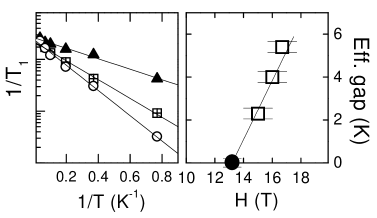
Figure 14: Left: activated behavior of $T^{-1}$ (line I) in the high field phase. Right: effective gap as a function of magnetic field. The intercept on the field axis coincide with the value of $H_{c2}=13.2\>T$.

7 Incommensurate phase and quantum critical regime

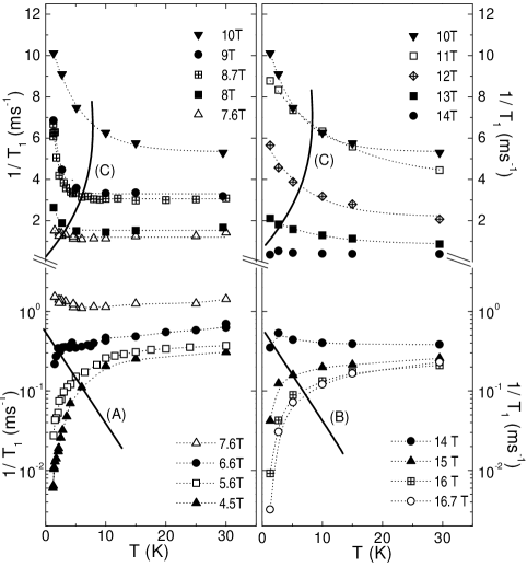
Figure 15: Left panel : temperature dependence of $1/T_{1}$ through the critical field $H_{c1}$. In the lower part, the $T_{1}^{-1}$ dependence in the singlet gapped phase ($H<H_{c1}$) is displayed, while its behavior in the magnetic phase ($H>H_{c1}$) is shown in the upper part. The dashed lines are guides to the eyes. Lines labeled (A) and (C) correspond to the crossover lines of Fig. 1. Right panel: temperature dependence of $1/T_{1}$ through the critical field $H_{c2}$. The upper part shows the behavior in the magnetic phase below $H_{c2}$ while the lower part is in the ”fully polarized” gapped phase ($H>H_{c2}$).

Fig. 15 gives the overall temperature and field dependence of the NMR relaxation rate (line I) through the entire phase diagram. In the left panel, the dependence of the $T_{1}^{-1}$ rate through the lower critical field is displayed. In the lower part, the behavior in the gapped phase is reproduced over a broader temperature range. Two distinct regimes can immediately be recognized. When the temperature is raised at constant field through the effective gap $\Delta_{-}$, the exponential suppression of the $T_{1}^{-1}$ crosses over to the temperature independent value of the relaxation rate expected in a classical system. Comparing with Fig. 1, this crossover can be recognized as line (A) (defined as $\mbox{$k_{\rm B}$}T=\Delta_{-}$) separating the gapped phase, controlled by quantum fluctuation, and the quantum critical phase where $\xi_{T}$ is the only relevant lengthscale. When the field is raised above $H_{c1}$, the behavior at high temperature is qualitatively the same but at low temperature $T_{1}^{-1}$ starts to diverge. Again, it is possible to place a crossover line (C) separating the two regimes. At high temperature, one recognizes the same quantum critical phase controlled solely by thermal fluctuation, while at low temperature, the spectrum of low energy fluctuation in the gapless magnetic phase controls the NMR relaxation. When the magnetic field is raised and crosses $H_{c2}$ (Fig. 15, right panel), the same features are qualitatively observed, with possibly a weaker divergence of $T_{1}^{-1}$ at low temperature in the gapless phase. What is the origin of this critical behavior of $T_{1}^{-1}$ throughout the gapless phase?

Because of the broken rotational symmetry, transverse (${\mathcal{S}}_{\perp}$) and longitudinal fluctuations (${\mathcal{S}}_{z}$) involve different processes (cf. Sec. 6) which do not have the same temperature dependence. Since staggered processes, entering ${\mathcal{S}}_{\perp}$, were found to dominate the $T_{1}^{-1}$ just below $H_{c1}$, it is natural to first examine the transverse low energy modes in the gapless phase. In the XXZ mapping for strongly coupled ladders (Sec. 4), two soft modes (transverse in the valence bond $\makebox[5.0pt]{ \put(0.0,-2.0){\line(0,1){9.0}} \put(0.0,-2.0){\circle*{2.5}} \put(0.0,7.0){\circle*{2.5}}},\makebox[5.0pt]{ \put(0.0,-2.0){\line(0,1){3.0}} \put(0.0,4.0){\line(0,1){3.0}} \put(0.0,-2.0){\circle*{2.5}} \put(0.0,7.0){\circle*{2.5}}}_{-1}$ basis) were found (Fig. 5). One mode is always at $Q=\pi$, and generates the staggered process which was already found to be strongly relevant. The other mode is at an incommensurate wavevector $Q_{\sigma}=\pi\sigma$, which is near $\pi$ when $H$ is close to $H_{c1}$ (top panel, Fig. 5). In Chitra97 , it was argued that this mode was gapped and did not contribute to transverse spin-spin correlation, in apparent contradiction with the spectrum of the XXZ model discussed in Sec. 4. On the other hand, this incommensurate soft mode in this model is a transverse singlet-triplet wave. For physically obscure reasons, the transverse spin-spin correlator in this state is indeed found to have zero spectral weight at the incommensurate wavevector. This point is crucial since it introduces a fundamental difference between spin-ladders and integer spin-chains which otherwise belong to the same universality class. This has also important consequences for neutron-scattering studies of spin-ladders. For NMR, the staggered process ($Q=\pi$) becomes the only relevant soft mode for (transverse) relaxation. If the temperature exceeds the maximum of the lower edge of the spectrum between $Q_{\sigma}=\pi\sigma$ and $\pi$ (Fig. 5, top panel), many additional modes contribute to ${\mathcal{S}}_{\perp}$. Hence the $Q=\pi$ soft mode is only relevant for temperature below the spin-stiffness constant $\rho_{s}$,

$$\rho_{s}\equiv\frac{\pi}{2}J_{\parallel}\frac{M}{M_{sat}}\approx\sqrt{J_{\parallel}g\mu_{B}(H-H_{c1})},$$ (23)

where the approximation is valid close to $H_{c1}$. The condition $kT\approx\rho_{s}$ specifies the crossover line between the ’Luttinger liquid’ and the quantum critical regime (Fig. 1 and 15 , line C). As the temperature is lowered, the spectral weight in the $Q=\pi$ soft mode increases giving the divergent contribution to

$$\frac{1}{T_{1}}\bigg{|}_{\perp}\propto\left(\frac{\rho_{s}}{\mbox{$k_{\rm B}$}T}\right)^{\eta-1},$$ (24)

where $\eta$ is the exponent governing the power law decay of the correlation functionsChitra97 . At $H_{c1}$ and $H_{c2}$, the exponent $\eta$ is known to be $\eta=1/2$ Sachdev94 and depends smoothly on the magnetization in between. The precise dependence of $\eta$ with $H$ is not known for ladders and could differ from Haldane systemsSakai91 , where the incommensurate mode at $Q_{\sigma}$ is relevant. The experimental $T_{1}^{-1}$ divergence observed at low temperature appears to be fully consistent with a square-root singularity (see Fig. 18). While there could also be additional critical fluctuations associated to the 3D ordering occurring at very low temperature, the divergence of $T_{1}^{-1}$ which is clearly noticeable below $5K$ ($\equiv 2J_{\parallel}$) has to involve 1D fluctuations.

At temperature above $\rho_{s}$, the relaxation rate gradually crosses over to a constant. This high temperature limit of the relaxation rate has a maximum around $10\>T$, field at which $g\mu_{B}H\approx J_{\perp}$.

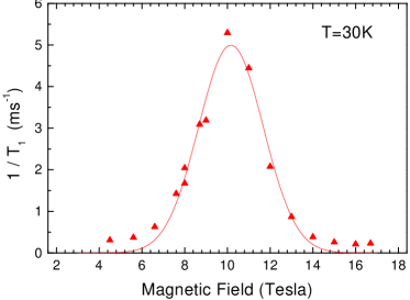
Figure 16: Field dependence of the longitudinal relaxation rate $T_{1}{-1}$ as a function of magnetic field. The maximum at $10$T is an independent measure of $J_{\perp}$.

In classical NMR theoryMoriya56 , the high temperature limit of the $T^{-1}$ relaxation rate is proportional to the second moment of the spectral distribution of excited states. This quantity is peaked precisely in the middle of the triplet band ($m_{z}=-1$). At high temperature where dimers are decorrelated, it is thereore natural to find a maximum in the relaxation rate as a function of field (shown in Fig. 16) at the level crossing between the $\makebox[5.0pt]{ \put(0.0,-2.0){\line(0,1){3.0}} \put(0.0,4.0){\line(0,1){3.0}} \put(0.0,-2.0){\circle*{2.5}} \put(0.0,7.0){\circle*{2.5}}}_{-1}$ and states. Since this ”classical” contribution is proportional to the zero frequency spectral weight, its temperature dependence is expected to be weak. It is anyway unrelated to the hydrodynamic soft mode at $Q=\pi$, which is a manifestation of the quasi long-range correlation along the ladder.

The longitudinal fluctuations (${\mathcal{S}}_{z}$) have also a contribution to the $T_{1}^{-1}$ relaxation rate originating from the $Q=0$ uniform mode. They have been shown to be non-criticalChitra97

$$\frac{1}{T_{1}}\bigg{|}_{\parallel}\propto\frac{\mbox{$k_{\rm B}$}T}{\rho_{s}}.$$ (25)

Since this contribution is noticeable only close to $H_{c1}$, where it is weak (see Fig. 15), it will not be discussed further.

Since in the experimental data shown in Fig. 15, we are clearly able to identify the scaling parameters $x_{<}=\Delta_{-}/\mbox{$k_{\rm B}$}T$ for $H<H_{c1}$ and $x_{>}=\rho_{s}/\mbox{$k_{\rm B}$}$ for $H>H_{c1}$ (line A and C) on each side of the critical field, it is natural to construct the scaling plots appropriate to this quantum critical point.

8 Scaling plots in the quantum critical regime

The concept of scaling at a quantum phase transition, one of the most beautiful idea in condensed matter physics, was developed in the context of the metal-insulator transition in disordered systemsAbrahams79 , where it has been brilliantly applied to doped semiconductorsPaalanen82 . But it is in two-dimensions that the concept has found the most spectacular applications: disordered superconducting films Haviland89 ; Hebard90 go directly from a superconducting to an insulating state through a $T=0$ quantum phase transition as a function of disorder. Josephson-junction arrays have a field tune vortex delocalization transition at a critical fraction of the flux quantum $f_{c}$Chen95 . In a two-dimensional electron gas, the transitions between quantum Hall plateaux or to a Hall-insulating stateShardar97 are also governed by zero temperature fixed pointsSondhi97 . More recently, the scaling properties of a novel metal-insulator transitionKravchenko96 in silicon MOSFET’s have also been thoroughly investigated. In light of this, it is surprising to find so few experimental studiesHaviland98 of quantum phase transitions in one dimension. On the other hand, many 1D systems have Lorentz invariance: this confers unique properties to their quantum critical points. In particular, their zero temperature critical behavior can be extended to any temperature via conformal mappingSachdev94 . This enables to give a precise description of the finite temperature ”quantum critical regime” discussed in the introduction, which is most easily revealed by a scaling analysis.

In the last section, the scaling parameters $x_{>}=\rho_{s}/\mbox{$k_{\rm B}$}$ and $x_{<}=\Delta_{-}/\mbox{$k_{\rm B}$}T$ above and below $H_{c1}$ have been identified using NMR. They are also appropriate to scale the magnetization curves (shown in Fig. 7): the resulting plot is shown in Fig. 17. Considering the overall quality of the scaling, the variable $x_{<}$ and $x_{>}$ are appropriate to this quantum critical point. Furthermore, the $0.42$K curve which crosses into the ordered phase just above $H_{c1}$ can also be included in this plot.

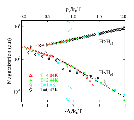
Figure 17: Magnetization scaling plot. Below $H_{c1}$ all curves collapse on a single curve when plotted in terms of the dimensionless scaling variable $(\Delta-g\mu_{B}H)/\mbox{$k_{\rm B}$}T$. As expected, the straight line with slope $-1$ for $x>1$ reproduces the exponential suppression of the magnetization with an effective gap $\Delta_{-}$ at low temperatures. Above $H_{c1}$, the scaling is also excellent (even in the ordered phase) using the parameter $\frac{\rho_{s}}{\mbox{$k_{\rm B}$}T}=\frac{\sqrt{g\mu_{B}(H-H_{c1})J_{\parallel}}}{\mbox{$k_{\rm B}$}T}$.

A similar scaling analysis of the longitudinal relaxation rate is also possible. Below $H_{c1}$, it is straightforward to scale all the experimental $T_{1}{-1}$ curves in terms of the single parameter $x_{<}$, as shown in Fig. 18 (lower curve). On this plot, the crossover line (A) shown on Fig 1 and 15 reduces to the single point $x=1$. For $x>1$, the exponentially activated behavior with energy $\Delta_{-}$ is the straight line shown with slope $-1$. Although all curves scale nicely for all $x$, the quantum critical regime is in principle limited to $\mbox{$k_{\rm B}$}T\leq 2J_{\parallel}$. Above $H_{c1}$, the appropriate scaling function is harder to construct because there are noncritical (classical) contributions to $T_{1}^{-1}$ which need to be subtracted. For all data shown on Fig. 15, these contributions were determined so that all curves have, after subtraction, the same asymptotic limit at high temperature. The field dependent constant $C(H)$ substracted was chosen to coincide with the single high-T value of $T_{1}^{-1}$ observed in the gapped phase ($H<H_{c1}$, $T\rightarrow\infty$) and is close to the high temperature limit of $T_{1}{-1}$ plotted in Fig. 16. In this way the $T\rightarrow\infty$ limit coincides with the $x_{<}=x_{>}=0$ point of the two scaling functions (above and below $H_{c1}$). After subtraction, all data for $H>H_{c1}$ also collapse on a unique scaling curve when expressed in terms of the scaling parameter $x_{>}$. Data points with $x>1$ are in the Luttinger liquid regime and a square-root divergence for $T_{1}^{-1}$ (line shown) agrees well with the experimental data. The precise scaling function can in principle be constructed for all $x$ from the zero temperature dynamicsChubukov94 and compared to this experimental scaling plot.

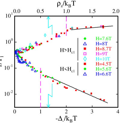
Figure 18: Scaling plot. Below $H_{c1}$ all the $T_{1}^{-1}$ measurements collapse on a single curve when plotted in terms of the dimensionless scaling variable $(\Delta-g\mu_{B}H)/\mbox{$k_{\rm B}$}T$. The point x=1 delimits the quantum critical regime from the quantum disordered phase. For $x>1$, the straight line with slope $-1$ drawn reproduces precisely the exponential suppression of the $T_{1}^{-1}$ rate. Above $H_{c1}$, after subtraction of a constant $C(H)$ to the $T_{1}^{-1}$ rate, it is possible to scale the remaining critical contributions to the $T_{1}^{-1}$ relaxation in terms of the scaling variable $\frac{\rho_{s}}{\mbox{$k_{\rm B}$}T}=\frac{\sqrt{g\mu_{B}(H-H_{c1})J_{\parallel}}}{\mbox{$k_{\rm B}$}T}$. In the Luttinger liquid regime ($x>1$), the data is consistent with a scaling function $R(x)=\sqrt{x}$ (solid line).

9 Conclusions

In this work, several clean experiments on spin-ladders have been used to illustrate the physics of quantum phase transitions. Much physical insight could be drawn using a mapping of strongly coupled ladders on a much studied model of quantum magnetism, the XXZ model. For a simple ladder, the anisotropy $\delta=J_{z}/J_{x}=1/2$ puts the system in the planar (X-Y) universality class between the critical fields $H_{c1}$ and $H_{c2}$. Any frustrating coupling (antiferromagnetic cross-bonding between legs) increases $\delta$. When $\delta>1$, the interactions between fermions (triplets bonds $\makebox[5.0pt]{ \put(0.0,-2.0){\line(0,1){3.0}} \put(0.0,4.0){\line(0,1){3.0}} \put(0.0,-2.0){\circle*{2.5}} \put(0.0,7.0){\circle*{2.5}}}_{-1}$) are very large and the system switches over to an Ising universality class with long range order. When an Ising gap is present, plateaux appear in the magnetization curve in the vicinity of $H_{\rm eff}=0$ ($\Leftrightarrow H=(H_{c1}+H_{c2})/2$, half filling), as the magnetic field has to overcome the Ising gap induced by the interactions. This problem has also been investigated theoretically by more general meansCabra97 . An interesting possibility raised in this paper is that similar physics could be induced by much smaller 3D antiferromagnetic coupling and may already have been observed in specific heat experimentsHammar98 ; Calemzuck98 on CuHpCl.

In the incommensurate gapless phase, low energy dynamical properties are dominated by the $Q=\pi$ soft mode in the transverse excitation spectrum (cf. Fig. 5). These fluctuations are not completely quenched in the gapped phase, since a three-magnons process, which can easily be identified by the temperature dependence of the NMR relaxation rateChaboussant97b , remains very strong close to $H_{c1}$ ($T_{1}^{-1}\propto\exp(-2\Delta_{-}/\mbox{$k_{\rm B}$}T)$). At finite temperature, spin-flip processes introduce a natural cutoff of the spin-spin correlations. When $\mbox{$k_{\rm B}$}T$ is larger than a characteristic quantum energy (the effective gap $\Delta_{-}$ below $H_{c1}$ or the spin-stiffness $\rho_{s}$ above $H_{c1}$), spin correlation have the same nature : this is the quantum critical regimeChubukov94 . All dynamical properties have in this limit a universal behavior which should be common to quantum phase transition in 1D with a continuous symmetry. The scaling properties of the NMR relaxation data on CuHpClChaboussant98 analyzed in this work should serve as a reference for future studies of 1D quantum critical points.

In spite of this almost idyllic picture, some questions remain open. In the gapless phase, the incommensurate soft mode should have observable consequences, probably requiring different experimental probes than the ones considered here. The nature of the low temperature ordered phase appears to hold the answer to several key issues in strongly correlated systems. One question to be answered is: can 1D quantum correlation persist in some form in 3D ordered phases? Finally, other compounds with more frustrated magnetic structures can potentially open new horizons in quantum magnetism: for example, there are new universality classes which have not been considered so far. There are indeed known modelsWaldtmann98 exhibiting an energy gap between singlet and triplet sectors but no gaps in the singlet sector. The experimental realization of such systems represents a unique challenge in this field.

The GHMFL is a Laboratoire Conventionné aux Universités J Fourier et INPG Grenoble I.

Appendix A: upper critical field

The energy of the fully polarized state $|f\rangle=|\uparrow,\uparrow,\ldots\rangle$ is

$$E_{F}=\langle F|{\mathcal{H}}|F\rangle=N\left(\frac{J_{\perp}}{4}+\frac{J_{\parallel}}{2}-g_{z}\mu_{B}H\right)$$

The most general state with one unit of angular momentum less than the completely polarized state is

$$|\psi\rangle=\sum_{j=1}^{N}\left(u_{j}S_{2j}^{-}+v_{j}S_{2j-1}^{-}\right)|F\rangle,$$ (26)

where the $u_{j}$ and $v_{j}$ are respectively the amplitude on the lower and upper legs. They are specified by the condition that $\psi\rangle$ should be an eigenstate of $\mathcal{H}$ with energy $E_{-}$, or equivalently

$$E_{F}-E_{-}=\sum_{j=1}^{N}\left[u_{j}S_{2j}^{-}+v_{j}S_{2j-1}^{-},{\mathcal{H}}\right]|F\rangle.$$ (27)

This condition yields a set of two coupled equations for the $u_{j}$ and $v_{j}$, which are easily solved in Fourier space. The dispersion relations for the corresponding spin-wave modes $\epsilon^{\alpha}(k)=E_{F}-E^{\alpha}_{-}(k)$ are

$$\epsilon^{o}(k) = g_{z}\mu_{B}H-J_{\parallel}(1-\cos k),$$ (28)

$$\epsilon^{a}(k) = g_{z}\mu_{B}H-J_{\perp}-J_{\parallel}(1-\cos k).$$ (29)

In the strong coupling limit, the ’acoustic’ mode (29) becomes soft first at wavevector $k=\pi$, when the field drops below the field which specifies $H_{c2}$ (12). It is straightforward to generalize the argument to more complex systems.

Appendix B: thermodynamics of the XXZ model

This problem has been completely set out by Takahashi and SuzukiTakahashi72 . For an anisotropy factor of $J_{z}/J_{x}=1/2$, all thermodynamic quantities can be computed from the solution of the coupled set of integral equations for the functions $\eta(x)$ and $\kappa(x)$,

$$\ln\eta(x) = 3\sqrt{3}\frac{J_{\parallel}}{\mbox{$k_{\rm B}$}T}+s(x)*\ln(1+u(x))$$

$$u(x) = 2\kappa(x)\cosh\frac{3g\mu_{B}H_{eff}}{2\mbox{$k_{\rm B}$}T}+\kappa^{2}(x)$$ (30)

$$\ln\kappa(x) = s(x)*\ln(1+\eta(x))$$ (31)

where $s(x)=\frac{1}{4}{\rm sech}\frac{\pi x}{2}$ and $*$ is the convolution product of two functions. For each value of the temperature and of the effective field, the thermodynamics is specified by the value $\kappa(0)$, i.e. the free-energy per spin is

$$\frac{F}{N}=-\frac{J_{\parallel}}{4}-\mbox{$k_{\rm B}$}T\ln\kappa(0).$$ (32)

We solved Eqs. (31) iteratively from the known solutions, $\eta(x)=3$ and $\kappa(x)=2$ for $J_{\parallel}=0$ and $H_{eff}=0$. We checked our results against the power series expansion in $J/T$Takahashi72

$$\frac{F}{N} = -\mbox{$k_{\rm B}$}T\ln\left(2\cosh\frac{g\mu H}{2\mbox{$k_{\rm B}$}T}\right)-\frac{J}{8}\frac{1}{\cosh^{2}\left(\frac{g\mu H}{2\mbox{$k_{\rm B}$}T}\right)}$$

$$- \frac{3J^{2}}{32\mbox{$k_{\rm B}$}T}\left\{\frac{1}{\cosh^{2}\left(\frac{g\mu H}{2\mbox{$k_{\rm B}$}T}\right)}-\frac{1/4}{\cosh^{4}\left(\frac{g\mu H}{2\mbox{$k_{\rm B}$}T}\right)}\right\}$$

The comparison with the experimental results shown in Fig. 7 is really excellent.

References

- (1) F.D.M. Haldane, Phys. Rev. Lett 50 (1983) 1153. F.D.M. Haldane, Phys. Lett. 93A, (1983) 464.
- (2) G. Chaboussant, P.A. Crowell, L.P. Lévy, O. Piovesana, A. Madouri, and D. Mailly, Phys. Rev. B 55, (1997) 3046.
- (3) G. Chaboussant, M.-H. Julien, Y. Fagot Revurat, L.P. Lévy, C. Berthier, M. Horvatić, and O. Piovesana, Phys. Rev. Lett. 79, (1997) 925.
- (4) G. Chaboussant, Y. Fagot-Revurat, M.-H. Julien, M.E. Hanson, C.Berthier, M. Horvatić, L.P. Lévy, and O. Piovesana, Phys. Rev. Lett 80 2713 (1998).
- (5) J.A. Hertz, Phys. Rev. B 14, (1976) 1165.
- (6) A.V. Chubukov, S. Sachdev and J. Ye, Phys. Rev. B 49, (1994) 11919.
- (7) S. Sachdev, T. Senthil and R. Shankar, Phys. Rev. B 50, (1994) 258.
- (8) S. Sachdev, Phys. Rev. B 55, (1997) 142.
- (9) S.L. Sondhi, S.M. Girvin, J.P. Carini, and D. Shahar, Rev. Mod. Phys. 69, 315 (1997).
- (10) R. Chitra and T. Giamiarchi, Phys. Rev. 55, (1997) 5816.
- (11) in Champs, Cordes et Phénomènes Critiques, E. Brézin and J. Zinn-Justin eds., Elsiever (1989).
- (12) L.P. Lévy in Magnétisme et Supraconductivité, Interéditions (1997), 232-238.
- (13) G.S. Uhrig and H.J. Schulz, Phys. Rev. B 54, (1996) 9624.
- (14) I. Affleck, T. Kennedy, E. Lieb and H. Tasaki, Phys. Rev. Lett. 59, (1987) 799.
- (15) K. M. Diederix, H. W. J. Blöte, J. P. Groen, T. O. Klaassen and N. J. Poulis, Phys. Rev. B 19 (1979) 420.
- (16) J.P. Renard, M. Verdaguer, L.P. Regnault, W.A.C. Erkelens, J. Rossat-Mignod and W.G. Sterling, Europhysics Lett. 3, (1987) 945 .
- (17) Y. Ajiro, T. Goto, H. Kikuchi, T. Sakakibara and T. Inami, Phys. Rev. Lett 63, (1989) 1424.
- (18) K. Katsumata, H. Hori, T. Takeuchi, M. Date, A. Yamagishi and J.P. Renard, Phys. Rev. Lett. 63, (1989) 86.
- (19) N. Fujiwara, T. Goto, S. Maegawa and T. Kohmoto, Phys. Rev. B 47, (1993) 11860.
- (20) E. Dagotto and T.M. Rice, Science 271, (1996) 618.
- (21) M. Azuma, Z. Hiroi, M. Takano, K. Ishida, and Y. Kitaoka, Phys. Rev. Lett. 73, (1994) 3463.
- (22) Z. Hiroi and M. Takano, Nature 377, (1995) 41.
- (23) B. Chiari, O. Piovesana, T. Tarentelli, and P.F. Zanazzi, Inorg. Chem. 29, (1990) 1172.
- (24) C. Hawyard, D. Poilblanc and L.P. Lévy, Phys. Rev. 54, (1996) 12649.
- (25) K. Totsuka, Phys. Rev. B 57 (1998) 3454.
- (26) F. Mila, cond-mat/9805029.
- (27) M. Reigrotzki, H. Tsunetsugu and T.M. Rice, J. Phys. C: Cond. Matt. 6, (1994) 9325.
- (28) P. Crowell, A. Madouri, M. Specht, G. Chaboussant D. Mailly and L.P. Lévy, Rev. Sci. Inst. 67, (1996) 4161.
- (29) Z. Weihong, R.R.P. Singh, J. Oitmaa, Phys. Rev. 55, (1997) 8052.
- (30) P.H. Hammar, D.H. Reich, C. Broholm and F. Trouw, Phys. Rev. B 57 (1998) 7846.
- (31) R. Calemzuck, et al., cond-mat/9805237.
- (32) C.N. Yang and C.P. Yang, Phys. Rev. 150, (1966) 321; ibid. 151, (1966) 258.
- (33) M. Takahashi and M. Suzuki, Prog. Theor. Phys. 48, (1972) 2187; M. Takahashi, Prog. Theor. Phys. 50, (1973) 1519.
- (34) M. Troyer, H. Tsunetsugu and D. Würtz, Phys. Rev. B 50, (1994) 13515.
- (35) Since all the high-energy states are excluded in the XXZ mapping, its validity is limited to temperatures below the .Similarly, the Zeeman splitting must be sufficiently large (say ) to avoid admixture with higher energy states.
- (36) A. Georges, private communication.
- (37) J. Sagi and I. Affleck, Phys. Rev. B 53, (1996) 9188.
- (38) T. Sakai and M. Takahashi, Phys. Rev. B 43, (1991) 13383.
- (39) Y. Fagot-Revurat, M. Horvatić, C. Berthier, P. Segransan, G. Dhalenne and A. Revcolecvshi, Phys. Rev. Lett. 77 (1996) 1861.
- (40) F.H.L. Essler, A.M. Tsvelik and G. Delfino, Phys. Rev. B 56 (1997) 11001.
- (41) T. Moriya, Prog. Theor. Phys. 16, (1956) 23.
- (42) E. Abrahams, P.W. Anderson, D.C. Licciardello and T.V. Ramakrishnan, Phys. Rev. Lett. 42, (1979) 673.
- (43) M.A. Paalanen, T.F. Rosenbaum, G.A. Thomas and R.N. Bhatt, Phys. Rev. Lett. 48, (1982) 284. T.F. Rosenbaum et al., Phys. Rev. B 27, (1983) 7509. H. Stupp, M. Hornung, M. Lakner, O. Madel, and H. v. Löhneysen, Phys. Rev. Lett. 71, (1993) 634. M.P. Sarachik et al., cond-matt/9706309.
- (44) D.B. Haviland, Y. Liu, and A.M. Goldman, Phys. Rev. Lett. 62, (1989) 2180.
- (45) A. F. Hebard and M.A. Paalanen, Phys. Rev. Lett. 65 (1990) 927.
- (46) C.D. Chen, P. Delsing, D.B. Haviland, Y. Harada, and T. Claeson, Phys. Rev. B 51, (1995) 15645.
- (47) D. Shardar, D.C. Tsui, M. Shayegan, E. Shimshomi, S.L. Sondhi, Phys. Rev. Lett. 79, (1997) 479. T. Wang, K.P. Clark, G.F. Spencer, A.M. Mack, and W.P. Kirk, Phys. Rev. Lett. 72, (1994) 709.
- (48) S.V. Kravchenko, D. Simonian, M.P. Sarachick, W. Mason, and J.E. Furneaux, Phys. Rev. Lett. 77, (1996) 4938. D. Popovic, A.B. Fowler, and S. Washburn, Phys. Rev. Lett. 79, (1997).
- (49) D. B. Haviland and P. Delsing, unpublished.
- (50) D. Cabra, A. Honecker, P. Pujol, Phys. Rev. Lett. 79, (1997) 5126 and cond-mat/9802035.
- (51) Ch. Waldtmann, H.-U. Everts, B. Bernu, P. Sindzingre, C. Lhuillier, P. Lecheminant and P. Pierre, cond-mat/9802168.