Phonons from neutron powder diffraction

Abstract

The spherically averaged structure function $S(|\mathbf{q}|)$ obtained from pulsed neutron powder diffraction contains both elastic and inelastic scattering via an integral over energy. The Fourier transformation of $S(|\mathbf{q}|)$ to real space, as is done in the pair density function (PDF) analysis, regularizes the data, i.e. it accentuates the diffuse scattering. We present a technique which enables the extraction of off–center ($|\mathbf{q}|\neq 0$) phonon information from powder diffraction experiments by comparing the experimental PDF with theoretical calculations based on standard interatomic potentials and the crystal symmetry. This procedure (dynamics from powder diffraction(DPD)) has been successfully implemented for two systems, a simple metal, fcc Ni, and an ionic crystal, CaF₂. Although computationally intensive, this data analysis allows for a phonon based modeling of the PDF, and additionally provides off–center phonon information from powder neutron diffraction.

For a variety of physical questions it is significant to obtain information on off-center phonons in crystals. This is particularly important in complex materials where local effects modify the macroscopic properties, as for example in high temperature superconductors, colossal magneto–resistive materials, ferroelectrics, intermetallic alloys and many more. Until this study the only available method to obtain off–center phonon data has been inelastic neutron scattering, which is intensity limited, hence time consuming, and for detailed studies, relies on the availability of large single crystals (triple axis measurements). Here we show how to obtain similar data from powder neutron diffraction.

Historically, the purpose of powder (polycrystalline) neutron diffraction has been the exact determination of the average crystal structure using modern crystallographic analysis techniques like Rietveld refinement, see e. g. [1]. Within this type of refinement only a limited range of the momentum transfer $q$ is necessary. More recently, however, the availability of pulsed sources has made possible the measurement of $S(|\mathbf{q}|)$ up to very large values of $q$. The PDF analysis [2] has made use of this additional information to investigate local atomic deviations from an average crystallographic structure.

To model the peak positions in the PDF analysis one calculates interatomic distances from the crystallographic unit cell. The peak shape is commonly fitted to the experimentally obtained PDF, $\rho^{exp}(r)$, using Gaussians. Since the experimental PDF contains additional information from the diffuse scattering, observed differences have been successfully attributed to local structural deformations like e. g. polarons [3]. This type of modeling of the PDF does not take into account the intrinsic peak widths caused by coherent excitations in solids like phonons or spin waves, and how the peak widths are modified by a finite momentum transfer cut–off. Other attempts to relate the measured PDF peak widths to the intrinsic phonon dynamics in a real space approach [4] were not intended to address the inverse problem, i. e. extracting the phonon parameters from the PDF. In a real space approach, it is considerably more difficult to take into account possible extinction rules for inelastic scattering caused by the point group symmetry of the reciprocal lattice, as has been recently shown [5]. Also in reciprocal space the instrumental resolution function is easier taken care of. In addition to information on lattice dynamics we provide an extended modeling of the PDF based on the estimated phonon parameters.

Triple axis neutron scattering is the most direct way to measure phonons. Indirect measurements on powders are either based on a detailed analysis of the peak shape in $S(|\mathbf{q}|)$, as is done in the analysis of thermal diffuse scattering (TDS) [6], or via a reconstruction of $S(|{\bf q}|,\omega)$ from time–of–flight (TOF) experiments, see e.g. [7]. Inelastic experiments are intensity limited, and the TDS analysis relies on a very good representation of the background. In this letter, we show how to extract information on off–center phonons in a reliable way from $S(|\mathbf{q}|)$ determined from TOF experiments. This is achieved via a parameterization of the phonon dispersion curves and eigenvectors using a suitable model (as is standard in the presentation of triple axis data, see e.g. [8, 9]), from which we can calculate a theoretical $S(|\mathbf{q}|)$. The data are then regularized by transforming to real space to obtain a theoretical PDF, $\rho^{theo}(r)$. A reverse Monte Carlo procedure is then used to estimate the parameters from a comparison with the experimental data, $\rho^{exp}(r)$, and to give data driven error bars.

The measured quantity is the powder (angular) averaged structure factor $S(|\mathbf{q}|)$ (normalized by the neutron scattering lengths). For simplicity we assume that the incoherent effects can be neglected, and decompose the total structure factor into elastic and one–phonon inelastic contributions: $S^{tot}_{coh}({\bf q})\approx S_{coh}^{elastic}({\bf q})+S_{coh}^{1}({\bf q})$. Note that $S^{tot}_{coh}(\mathbf{q})$ contains all dynamic information as an integral over frequency[10]. The elastic part is given by [11]

$$S_{coh}^{elastic}({\bf q})=\frac{(2\pi)^{3}}{N_{b}v_{0}}\frac{1}{\overline{b}^{2}}\sum_{{\bf G},d}\delta({\bf q}-{\bf G})\overline{b}_{d}e^{i{\bf q}.{\bf d}-W_{d}({\bf q})}$$ (1)

and the one–phonon inelastic part by

$$S_{coh}^{1}({\bf q}) = \frac{\hbar(2\pi)^{3}}{2N_{{\bf k}}N_{b}v_{0}}\frac{1}{\overline{b}^{2}}\sum_{{\bf G}}\sum_{{\bf k}\in BZ,j}\left|F_{j}({\bf q})\right|^{2}$$ (2)

$$\times \delta({\bf q}-{\bf G}+{\bf k})\frac{\coth(\frac{\beta}{2}\hbar\omega_{{}_{j}}({\bf k}))}{\omega_{j}({\bf k})}\;,$$

where $F_{j}({\bf q})=\sum_{d}\frac{\overline{b_{d}}}{\sqrt{M_{d}}}({\bf q}.\boldsymbol{\sigma}^{j}_{d}({\bf k}))e^{-W_{d}({\bf q})+i{\bf q}.{\bf d}}$, the sum over $\mathbf{G}$ runs over all vectors of the reciprocal lattice, $\mathbf{k}$ describes a Brillouin zone integral over $N_{{\bf k}}$ points, $d$ runs over atoms in the cell and $j$ counts the branches. $\overline{b_{d}}$ is the average scattering length and $M_{d}$ the mass of the $d$’th atom, $v_{0}$ the unit cell volume, and $W(\mathbf{q})$ is the Debye-Waller factor defined as $W_{d}({\bf q})=\frac{\hbar}{4N_{k}M_{d}}\sum_{{\bf k}\in BZ,j}\frac{\left|{\bf q}.\boldsymbol{\sigma}^{j}_{d}({\bf k})\right|^{2}}{\omega_{j}({\bf k})}\coth(\frac{\beta\hbar}{2}\omega_{j}({\bf k}))\;$. The phonons enter eqns (1) and (2) via the dispersion relations $\omega_{j}(\mathbf{k})$ and the eigenvectors $\boldsymbol{\sigma}_{d}^{j}(\mathbf{k})$. The powder averaged structure function $S(|{\bf q}|)\equiv\frac{1}{4\pi}\int_{|{\bf q}|=const}d\Omega_{{\bf q}}\>S(\mathbf{q})$ must be obtained numerically, and is CPU time consuming for the inelastic part of eqn(2). To compare to the experimental situation it is necessary to convolute $S(|\mathbf{q}|)$ with a suitably chosen resolution function[2] which depends on the instrument.

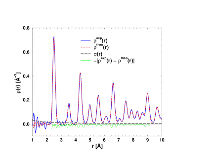
FIG. 1.: The experimental $\rho^{exp}(r)$ compared with the theoretical $\rho^{theo}(r)$ calculated for the expectation values $\{\overline{f_{i}}\}$ resulting from the DPD procedure for Ni at room temperature. $\sigma(r)$ are the experimental errors in the $\chi^{2}$ estimator (4).

The extraction of the lattice dynamics described by $\omega_{j}({\bf q})$ and $\boldsymbol{\sigma}_{d}^{j}({\bf q})$ using a comparison of TOF experimental data with a theoretical $S(|\mathbf{q}|)$ is difficult in reciprocal space because $S(|\mathbf{q}|)$ is a superposition of elastic scattering, i.e. the Bragg peaks, and inelastic scattering, both of which are vastly different in amplitude. A direct comparison in reciprocal space is further complicated by the unavoidable instrument background which is superimposed on the data. Both problems can be greatly reduced by transforming $S(|\mathbf{q}|)$ into the real space pair density function $\rho(r)$ via Fourier transform

$$\rho(r)=\rho_{0}+\frac{1}{2\pi^{2}r}\int_{0}^{\infty}dq\>\left[S(|{\bf q}|)-1\right]q\sin(qr)\;.$$ (3)

Pulsed sources provide a high enough momentum transfer to reduce the truncation error in eqn (3) and in turn, allow for a proper normalization of the data. Due to the properties of a Fourier transform the peaks in $\rho(r)$ are all of comparable height which eliminates the problem with the large amplitude fluctuations in $S(|\mathbf{q}|)$, i.e. it regularizes the data analysis problem. As a useful byproduct, all features in $S(|\mathbf{q}|)$ with inverse length scales larger than $\frac{2\pi}{a_{0}}$, i.e. most of the background, are transformed into distances in $\rho(r)$, which are smaller than the shortest interatomic distance $a_{0}$, and can therefore be neglected in the parameter estimation.

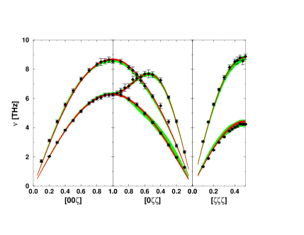
FIG. 2.: The phonon dispersion curves for room temperature Ni. The symbols are triple axis data from [13]. The shaded bands are the one–sigma error intervals of the dispersion curves obtained by our procedure. The green bands result from just reproducing the PDF, and the red bands are from constraining the reverse Monte Carlo to agree with the measured elastic constants within their error bars.

We use a $\chi^{2}$–functional in the parameter estimation process defined by

$$\chi^{2}\left(\{f_{i}\}\right)=\int_{r_{a}}^{r_{b}}dr\>\frac{\left[\rho^{exp}(r)-\rho^{theo}(r;\{f_{i}\})\right]^{2}}{\sigma(r)^{2}}\;$$ (4)

where $\sigma(r)$ is the error in $\rho^{exp}(r)$, which can be assumed to be $\frac{\sigma_{0}}{r}$ [2]. The variational parameters are the parameters describing the lattice dynamics $\{f_{i}\},$ which depend on a theoretical model (see below for concrete examples). $r_{a}$, $r_{b}$ define the range over which the PDFs are compared. We use a Monte Carlo procedure [12] which gives statistical estimators for the parameters $\overline{f_{i}}$, and also error bars $(\Delta f_{i})^{2}\equiv{\overline{f_{i}^{2}}-\overline{f_{i}}^{2}}$. The $\Delta f_{i}$ are controlled by the quality of the phonon model (a bad model also giving a large $\chi^{2}$, i.e. systematic error), and by the quality of the data, the statistical error. Due to the nature of our data, the experimental PDF, the dynamics is obtained by averaging over the whole reciprocal space, not just along symmetry directions, as is usually done, when triple axis data are fitted.

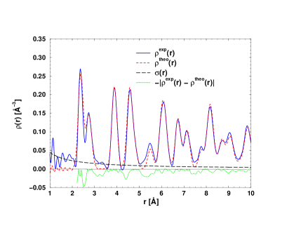
FIG. 3.: The same as Fig. 1 but for $CaF_{2}$ at room temperature.

The parameterization of the lattice dynamics involves the choice of a theoretical model. There exists a large variety of models which describe the measured dispersions from triple axis data [8, 9]. To validate our procedure we chose to perform the above analysis on two materials with very different models for the lattice dynamics. The first example is fcc Ni, whose phonon dispersion can be described by a simple force constant model [13, 14]. In Fig. 1, the PDF determined from the diffraction data is compared with the PDF calculated from the estimated parameters. The agreement is excellent and indicates that this procedure does indeed reproduce both the peak position and peak shape of a PDF measurement. A comparison of the force constants resulting from our analysis with existing triple axis data is shown in Table 1. Given the force constants and their standard deviations we can easily calculate the resulting phonon dispersion curves. In Fig. 2 we show those curves together with published triple axis data [13]. Again the agreement is excellent proving that we managed to extract the dynamical information contained in $S(|\mathbf{q}|)$. Adding more information, e.g elastic constants, to the functional (4) reduces the errors in our parameter estimation. The additional constraints lead to smaller error bars, and a slight improvement in the overall shape of the dispersions.

As a second example we took $CaF_{2}$, since it involves a fairly ionic system, which necessitates a different interatomic force model. Also the phonons are a lot more complicated due to the presence of optical branches. The phonons were parameterized by ionic shell models, as described in Elcombe & Pryor [15]. This is a more challenging problem as we now have a much higher dynamic range (phonon energies up to $14$THz ), and the optical modes show an unusually large dispersion. The results of the DPD analysis are presented together with some available triple axis data in Table 2 for the force constants, and in Figs. 3 and 4 for the comparison of PDFs and dispersions, respectively. Again, the agreement is remarkable and shows that we can obtain reliable off-center phonon information even for non-trivial systems.

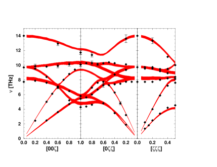
FIG. 4.: The phonon dispersion curves for $CaF_{2}$ at room temperature. The symbols are measured data from [16]. The shaded bands are one–sigma intervals of the dispersion curves obtained by our procedure. .

In this letter we have shown how dynamical information present in $S(|\mathbf{q}|)$ data can be extracted. The success of the present analysis relies on high quality data and on intelligent modeling of the lattice dynamics. Noisy data or bad normalization will result in large error bars. The models can easily be extended and modified if the error analysis indicates through an unusually large $\chi^{2}$-value that the model is incompatible to the data. Such extensions may include more shells, or a totally different modeling based on pseudopotential calculations. As additional constraints to the functional in eqn.(4) we can use further data from zone center experiments, like elastic constants and Raman data. At very low temperatures where the one-phonon processes are not thermally activated, the information is not in the data. If necessary, more sophisticated Placzek corrections and the incoherent scattering can be included in the analysis. Our results are very encouraging, and we will pursue this effort on more complicated materials, where triple axis data are sparse or non-existent.

TABLE I.: Generalized force constants $f\pm\Delta f$ for Ni at room temperature (in $10^{4}$ dyn/cm) from reverse Monte Carlo runs with (a) the elastic constants constraints, (b) without , and from a triple-axis measurement Ref. [14]. The errors in the force constants in Ref. [14] are estimated at about $\pm 0.04\times 10^{4}$ dyn/cm. The notation follows Ref. [14].

	(a)				(b)				Ref. [14]
1XX	1	.755 ${}\pm{}$	0	.018	1	.683 ${}\pm{}$	0	.024	1	.7319
1ZZ	-0	.054 ${}\pm{}$	0	.019	-0	.039 ${}\pm{}$	0	.019	-0	.0436
1XY	1	.878 ${}\pm{}$	0	.017	1	.869 ${}\pm{}$	0	.159	1	.9100
2XX	0	.067 ${}\pm{}$	0	.023	0	.122 ${}\pm{}$	0	.046	0	.1044
2YY	-0	.011 ${}\pm{}$	0	.008	-0	.085 ${}\pm{}$	0	.031	-0	.0780
3XX	0	.071 ${}\pm{}$	0	.007	0	.102 ${}\pm{}$	0	.013	0	.0842
3YY	0	.031 ${}\pm{}$	0	.004	0	.044 ${}\pm{}$	0	.006	0	.0263
3XZ	0	.045 ${}\pm{}$	0	.001	0	.027 ${}\pm{}$	0	.020	0	.0424
3YZ	-0	.010 ${}\pm{}$	0	.005	-0	.009 ${}\pm{}$	0	.005	-0	.0109

TABLE II.: The parameters of the shell model used for CaF₂. The notation follows Ref. [15] and the ionic charge Z(Ca) was fixed at $2e$ (shell model III in Ref. [15]).

	Units	RMC of PDF				Ref. [15]
$A_{1}$	$e^{2}/v$	16	.00 ${}\pm{}$	0	.25	15	.12 ${}\pm{}$	0	.17
$B_{1}$		-1	.84 ${}\pm{}$	0	.09	-1	.70 ${}\pm{}$	0	.08
$A_{2}$		1	.30 ${}\pm{}$	0	.11	1	.30 ${}\pm{}$	0	.11
$B_{2}$		0	.09 ${}\pm{}$	0	.01	0	.09 ${}\pm{}$	0	.03
$A_{3}$		0	.22 ${}\pm{}$	0	.02	0	.23 ${}\pm{}$	0	.17
$B_{3}$		-0	.28 ${}\pm{}$	0	.03	-0	.28 ${}\pm{}$	0	.06
$A_{4}$		-0	.18 ${}\pm{}$	0	.02	-0	.18 ${}\pm{}$	0	.04
$B_{4}$		0	.062 ${}\pm{}$	0	.006	0	.061 ${}\pm{}$	0	.014
$\alpha$(Ca)	$e$	1	.66 ${}\pm{}$	0	.16	1	.63 ${}\pm{}$	0	.11
$d$(Ca)	$\AA^{3}$	-0	.25 ${}\pm{}$	0	.02	-0	.25 ${}\pm{}$	0	.03
$\alpha$(F)	$e$	0	.45 ${}\pm{}$	0	.04	0	.45 ${}\pm{}$	0	.04
$d$(F)	$\AA^{3}$	0	.065 ${}\pm{}$	0	.006	0	.063 ${}\pm{}$	0	.015

REFERENCES

- [1] Edited by R. A. Young, The Rietveld Method (Oxford University Press, Oxford, 1993).
- [2] T. Egami, Mater. Trans 31, 163 (1990); B. H. Toby and T. Egami, Acta Cryst. A 48, 336 (1991).
- [3] D. Louca et al., Phys. Rev. B 56, R8475 (1997); D. Louca, G. H. Kwei, and J. F. Mitchel, Phys. Rev. Lett. 80, 3811 (1998).
- [4] J. S. Chung and M. F. Thorpe, Phys. Rev. B 55, 1545 (1997).
- [5] J. M. Perez–Mato et al., Phys. Rev. Lett. 82, 2462 (1998).
- [6] P. Schofield and B. T. M. Willis, Acta Cryst. A 43, 803 (1987), C. J. Carlisle and B. T. M. Willis, Acta Cryst. A 45, 708 (1989).
- [7] U. Buchenau, H. R. Schober, and R. Wagner, Journal de Physique C6, 395(1981); U. Buchenau et al., Phys. Rev. B 27, 955 (1983); M. Heiroth et al., Phys. Rev. B 34, 6681 (1986).
- [8] H. Biltz and W. Kress, Phonon Dispersion Relations in Insulators (Springer Verlag, New York, 1979).
- [9] Landolt–Börnstein, Numerical Data and Functional Relationships in Science and Technology (Springer Verlag, Berlin, 1974), Vol. V13a.
- [10] The data that we are using are obtained from TOF measurements at the IPNS on the GLAD diffractometer and MLNSC on the HIPD diffractometer, where the information is calculated assuming elastic scattering with Placzek corrections (In G. L. Squires, Introduction to the Theory of Thermal Neutron Scattering, Dover, New York, 1996).
- [11] S. W. Lovesey, Theory of Neutron Scattering from Condensed Matter (Clarendon Press, Oxford, 1985), Vol. 1.
- [12] R. L. McGreevy, Nucl. Inst. and Meth. A 354, 1 (1995).
- [13] R. J. Birgeneau, J. Cordes, G. Dolling, and A. D. B. Woods, Phys. Rev. 136, A1359 (1964).
- [14] G. A. DeWit and B. Brockhouse, J. Appl. Phys. 39, 451 (1968).
- [15] M. M. Elcombe and A. W. Pryor, J. Phys. C 3, 492 (1970).