Ground state instability in systems of strongly interacting fermions

Abstract

We analyze stability of a fermion system with model repulsive pair interaction potential. The possibility for different types of restructuring of the Fermi ground state (at sufficiently great coupling constant) is related to the analytic properties of such potential. In particular, for the screened Coulomb law it is shown that the restructuring cannot be of the Fermi condensation type, known earlier for some exactly solvable models, and instead it belongs to the class of topological transitions (TT). For this model, a phase diagram has been built in the variables ”screening parameter - coupling constant” which displays two kinds of TT: a ${}^{5}/_{2}$-kind similar to the known Lifshitz transitions in metals, and a 2-kind characteristic for a uniform strongly interacting system.

PACS: 71.10.-w, 71.10.Hf

The common ground state of isotropic Fermi gas with density $\rho$ is described (at zero temperature) by the stepwise Fermi function $n_{{\textrm{F}}}(p)=\theta(p_{{\textrm{F}}}-p)$, dropping discontinuously from 1 to 0 at the Fermi momentum $p_{{\textrm{F}}}=(3\pi^{2}\rho)^{1/3}$ (in the units where $\hbar=1$). The Landau theory of an interacting Fermi liquid started from the assumptions that the quasiparticle distribution function $n(p)$ coincides with the one of an ideal gas, while the single particle spectrum $\varepsilon_{p}$ is similar to that of ideal gas, being characterized by the effective mass $M^{*}$ [1].

But these $n_{{\textrm{F}}}(p)$ and $\varepsilon_{p}$ can be broken down under certain circumstances. The best known example is the Cooper pairing at arbitrarily weak attractive interaction with subsequent formation of the pair condensate and gapped quasiparticle spectrum [2], but also a repulsive interaction, if sufficiently strong, can produce non-trivial ground states. The first example of such restructuring for a Fermi system with model repulsive interaction [3] revealed existence of a critical value $\alpha_{cr}$ for the interaction constant $\alpha$, such that at $\alpha=\alpha_{cr}$ the stability criterion $s(p)=(\varepsilon_{p}-\varepsilon_{{\textrm{F}}})/(p^{2}-p_{{\textrm{F}}}^{2})>0$ fails just at the Fermi surface: $s(p_{{\textrm{F}}})=0$ ($p_{{\textrm{F}}}$-instability). Then at $\alpha>\alpha_{cr}$ an exact solution exists of a variational equation for $n(p)$ (following from the Landau energy functional $E[n(p)]$), exhibiting a certain finite interval $(p_{1},p_{2})$ around $p_{{\textrm{F}}}$ where the distribution function $n(p)$ varies continuously and takes intermediate values between $1$ and $0$, while the single-particle excitation spectrum $\varepsilon_{p}$ has a flat plateau,

$$\frac{\delta E[n(p)]}{\delta np)}=\varepsilon_{p}=\mu;\;\;\;p_{1}\leq p\leq p_{2},$$ (1)

with $\mu$ being the chemical potential. It is seen from eq. (1) that the occupation numbers $n(p)$ become variational parameters, deviating from the Fermi function in order to minimize the energy $E$. This phenomenon was called fermion condensation (FC) and soon several model forms for $E[n(p)]$ were proposed [4]-[8] providing similar solutions. However, these models do not answer the question whether there exist other types of phase transitions related to a rearrangement of the Fermi function $n_{{\textrm{F}}}(p)$ and the single particle spectrum $\varepsilon_{p}$. It is pertinent to note that the idea of multiconnected Fermi sphere, with production of new, interior segments of the Fermi surface, has been considered already [9, 10]. This determines an interest to examine the overcritical regimes $\alpha>\alpha_{cr}$ for the models displaying alternative types of instability.

The main goal of this Letter is to consider possible types of rearrangement of the Fermi ground state. We shall relate the types of such rearrangement to analytic properties of the single particle potential of a system in question and show that there can exist phase transitions of different type from FC.

The general scheme of Refs. [3]-[7] for a homogeneous system of non-polarized fermions with mass $M$ and model isotropic interaction potential $U(p)$ considers the energy functional $E[n(p)]$:

$$E[n(p)]=\int\frac{p^{2}}{2M}n(p)\frac{d{\textbf{p}}}{(2\pi)^{3}}+\frac{1}{2}\int\int n(p)U(|{\textbf{p}}-{\textbf{p}}^{\prime}|)n(p^{\prime})\frac{d{\textbf{p}}d{\textbf{p}}^{\prime}}{(2\pi)^{6}},$$ (2)

and the related quasiparticle dispersion law:

$$\varepsilon_{p}=\frac{p^{2}}{2M}+\int U(|{\textbf{p}}-{\textbf{p}}^{\prime}|)n(p^{\prime})\frac{d{\textbf{p}}^{\prime}}{(2\pi)^{3}}.$$ (3)

Performing the angular integration and passing to the dimensionless variables: $x=p/p_{{\textrm{F}}}$, $y=2M\varepsilon_{p}/p_{{\textrm{F}}}^{2}$, $z=2\pi^{2}ME/p_{{\textrm{F}}}^{5}$, eqs. (2,3) can be presented in a simpler form:

$$z[\nu(x)]=\int[x^{4}+\frac{1}{2}x^{2}V(x)]\nu(x)dx,$$ (4)

$$y(x)=x^{2}+V(x),$$ (5)

with the single particle potential $V(x)$ being given by,

$$V(x) = \frac{1}{x}\int x^{\prime}\nu(x^{\prime})u(x,x^{\prime})dx^{\prime},$$ (6)

$$u(x,x^{\prime}) = \frac{M}{\pi^{2}p_{F}}\int\limits_{|x-x^{\prime}|}^{x+x^{\prime}}u(t)tdt.$$

Here $u(x)\equiv U(p_{{\textrm{F}}}x)$, and the distribution function $\nu(x)\equiv n(p_{{\textrm{F}}}x)$ is positive, obeys the normalization condition:

$$\int x^{2}\nu(x)dx=1/3,$$ (7)

and the Pauli principle limitation $\nu(x)\leq 1$. The latter can be lifted using, e.g., the ansatz: $\nu(x)=$ $[1+\tanh\eta(x)]/2$, then the system ground state should correspond to the minimum of the functional:

$$f[\eta(x)]=\int[1+\tanh\eta(x)]\{x^{4}-\mu x^{2}+\frac{1}{4}x\int x^{\prime}[1+\tanh\eta(x^{\prime})]u(x,x^{\prime})dx^{\prime}\}dx,$$ (8)

containing a Lagrange multiplier $\mu$, with respect to an arbitrary variation of the auxiliary function $\eta(x)$. This permits to present the necessary condition of extremum $\delta f=0$ as:

$$x^{2}\nu(x)[1-\nu(x)][y(x)-\mu]=0,$$ (9)

which means that either $\nu(x)$ takes only the values $0$ and $1$ or the dispersion law is flat [3]: $y(x)=\mu$, in accordance with eq. (1). The last possibility just corresponds to FC. As it is seen from eq. (1), the single particle spectrum $\varepsilon_{p}$ in this case cannot be analytic function of complex $p$ in any open domain, containing the FC interval $\Delta p=[p_{1},p_{2}]$. In fact, all the derivatives of $\varepsilon_{p}$ with respect to $p$ should be zero along $\Delta p$, while this is not the case along the real axis outside $\Delta p$. For instance, in the FC model with $U(p)=U_{0}/p$ [3] the kernel, eq. (6), results non-analytic:

$$u(x,x^{\prime})=\frac{MU_{0}}{\pi^{2}p_{{\textrm{F}}}}(x+x^{\prime}+|x-x^{\prime}|)$$ (10)

which eventually causes non-analyticity of the potential $V(x)$.

On the other hand, as it follows from eq. (5), the single particle spectrum will be an analytic function along the whole real axis, provided $V(x)$ is such a function. In this case FC is forbidden and the only alternative to the Fermi ground state (if the stability criterion gets broken) leaves in a topological transition (TT) between the topologically unequal states with $\nu(x)=0,1$ [12]. Generally, all such states are classified by the indices of connectedness (known as Betti numbers in algebraic topology [13]) for the support of $\nu(x)$. In fact, for an isotropic system, these numbers are simply to count the separate (concentric) segments of the Fermi surface. Then the system ground state will correspond to such a multiconnected distribution (Fig. 1):

$$\nu(x)=\sum_{i=1}^{n}\theta(x-x_{2i-1})\theta(x_{2i}-x),\,$$ (11)

that the parameters $0\leq x_{1}<x_{2}<\ldots<x_{2n}$ obey the normalization condition:

$$\sum_{i=1}^{n}(x_{2i}^{3}-x_{2i-1}^{3})=1,$$ (12)

and the related $z$, eq. (4),

$$z=\frac{1}{2}\sum_{i=1}^{n}\int\limits_{x_{2i-1}}^{x_{2i}}x^{2}[x^{2}+y(x)]dx$$ (13)

has the absolute minimum with respect to $x_{1},\ldots,x_{2n-1}$ and to $n\geq 1$.

\psfrag{v}[3]{$\nu(x)$}\psfrag{1}[3]{1}\psfrag{0}[3]{0}\psfrag{a}[t][3]{$x_{1}$}\psfrag{b}[t][3]{$x_{2}$}\psfrag{c}[t][3]{$x_{3}$}\psfrag{d}[t][3]{$x_{4}$}\psfrag{e}[t][3]{$x_{2n-1}$}\psfrag{f}[t][3]{$x_{2n}$}\psfrag{h}[3]{$\cdots$ }\includegraphics{fig1.eps}

Figure 1: Occupation function for a multiconnected distribution.

Differentiating eq. (13) in the parameters $x_{1},\ldots,x_{2n-1}$ with use of the relations:

$$\frac{{\partial}x_{2n}}{{\partial}x_{k}}=(-1)^{k-1}(\frac{x_{k}}{x_{2n}})^{2},\,\,\,1\leq k\leq 2n-1,$$ (14)

by virtue of eq. (12), and taking into account that the potential $V(x)$ in the dispersion law $y(x)$ in fact also depends on these parameters:

$$V(x)=\frac{1}{x}\sum_{i=1}^{n}\int_{x_{2i-1}}^{x_{2i}}x^{\prime}u(x,x^{\prime})dx^{\prime},$$ (15)

we present the necessary conditions of extremum as:

$$\frac{{\partial z}}{{\partial}x_{k}}=(-1)^{k}x_{k}^{2}[y(x_{k})-y(x_{2n})]=0,\,\,\,1\leq k\leq 2n-1.$$ (16)

Hence the multiconnected ground state is controlled by the evident rule of unique Fermi level: $y(x_{k})=y(x_{2n})$, for all $1\leq k\leq 2n-1$ (except for $x_{1}=0$). In principle, given the kernel $u(x,x^{\prime})$ all the $(2n-1)$ unknown parameters $x_{k}$ can be found from eqs. (16,5,15). Then, the sufficient stability conditions: $\partial^{2}z/\partial x_{i}\partial x_{j}=\alpha_{i}\delta_{ij}$, $\alpha_{i}>0$, provide the generalized stability criterion: the dimensionless function

$$\sigma(x)=2Ms(p)=\frac{y(x)-y\left(x_{2n}\right)}{x^{2}-x_{2n}^{2}}$$ (17)

should be positive within filled and negative within empty intervals, turning zero at their boundaries in accordance with eqs. (16). It can be proved rigorously that for given analytic $u(x,x^{\prime})$ this criterion uniquely defines the system ground state.

In what follows we shall label each multiconnected state, eq. (11), by an entire number related to the binary sequence of empty and filled intervals read from $x_{2n}$ to $0$. Thus, the Fermi state with a single filled interval $[x_{2}=1,\;x_{1}=0]$ reads as unity, the state with a void at origin: (filled $[x_{2},\;x_{1}]$ and empty $[x_{1},\;0]$) reads as $(10)=2$, the state with a single gap: $(101)=3$, etc. Note that all even phases have a void at the origin and odd phases have not.

For free fermions $V(x)=0$, $y(x)=x^{2}$, eqs. (16) only yield the trivial solution corresponding to the Fermi state $1$. In order to pass to non-trivial realizations of TT, we choose $U(p)$ corresponding to the common screened Coulomb potential:

$$U(p)=\frac{4\pi e^{2}}{p^{2}+p_{0}^{2}}.$$ (18)

The related explicit form for the kernel

$$u(x,x^{\prime})=\alpha\ln\frac{(x+x^{\prime})^{2}+x_{0}^{2}}{(x-x^{\prime})^{2}+x_{0}^{2}},$$ (19)

with the dimensionless screening parameter $x_{0}=p_{0}/p_{{\textrm{F}}}$ and the coupling constant $\alpha=2Me^{2}/\pi p_{{\textrm{F}}}$, evidently displays the necessary analytical properties for existence of TT.

With use of eqs. (15) and (19), the potential $V\left(x\right)$ is expressed in elementary functions:

$$V(x)=\sum_{i=1}^{n}V(x;x_{2i-1},x_{2i}),$$ (20)

$$V(x;x^{\prime},x^{\prime\prime})=\alpha\left\{2\left[x^{\prime\prime}-x^{\prime}-x_{0}\arctan\frac{2x_{0}\left(x^{\prime\prime}-x^{\prime}\right)\left(x^{2}+x_{0}^{2}+x^{\prime}x^{\prime\prime}\right)}{\left(x^{2}+x_{0}^{2}-x^{\prime 2}\right)\left(x^{2}+x_{0}^{2}-x^{\prime\prime 2}\right)}\right]\right.+$$

$$\left.+\frac{1}{2x}\left[\left(x^{\prime\prime 2}+x_{0}^{2}-x^{2}\right)\ln\frac{\left(x+x^{\prime\prime}\right)^{2}+x_{0}^{2}}{\left(x-x^{\prime\prime}\right)^{2}+x_{0}^{2}}-\left(x^{\prime 2}+x_{0}^{2}-x^{2}\right)\ln\frac{\left(x+x^{\prime}\right)^{2}+x_{0}^{2}}{\left(x-x^{\prime}\right)^{2}+x_{0}^{2}}\right]\right\}.$$

Then, the straightforward analysis of eqs. (16) shows that their non-trivial solutions only appear when the coupling parameter $\alpha$ exceeds a certain critical value $\alpha^{*}$. This corresponds to the moment when the stability criterion [3] $\sigma(x)=(y_{{\textrm{F}}}(1)-y_{{\textrm{F}}}(x))/(1-x^{2})>0$ calculated with the Fermi distribution, $y_{{\textrm{F}}}(x)=x^{2}+V(x;0,1)$, fails in a certain point $0\leq x_{i}<1$ within the Fermi sphere: $\sigma(x_{i})\to 0$. There are two different types of such instability depending on the screening parameter $x_{0}$ (Fig. 2). For $x_{0}$ below certain threshold value $x_{th}\approx 0.32365$ (weak screening regime, WSR) the instability point $x_{i}$ sets rather close to the Fermi surface: $1-x_{i}\ll 1$, while it drops in a critical way to zero at $x_{0}\to x_{th}$ and pertains zero for all $x_{0}>x_{th}$ (strong screening regime, SSR). The critical coupling $\alpha^{*}(x_{0})$ results a monotonically growing function of $x_{0}$, having the asymptotics $\alpha^{*}(x_{0})\approx\left(\ln 2/x_{0}-1\right)^{-1}$at $x_{0}\to 0$ and staying analytic at $\alpha_{th}=\alpha^{*}(x_{th})\approx 0.91535$, where it only exhibits an inflexion point.

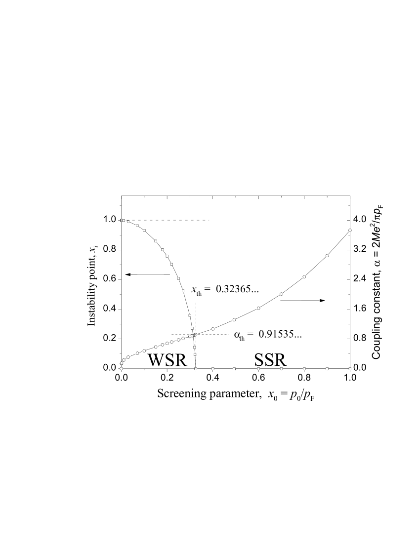
Figure 2: Critical coupling $\alpha^{*}$ and instability point $x_{i}$ as functions of screening. The regions of weak screening (WSR) and strong screening (SSR) are separated by the threshold value $x_{th}$ (note that $x_{th},\,\alpha_{th}$ is the triple point between the phases 1, 2, 3 in Fig. 3).

These two types of instability give rise to different types of TT from the state $1$ at $\alpha>\alpha^{*}$: at SSR a void appears around $x=0$ ($1\to 2$ transition), and at WSR a gap opens around $x_{i}$ ($1\to 3$ transition). Further analysis of eqs. (16) shows that the point $x_{th},\;\alpha_{th}$ represents a triple point in the phase diagram in variables $x_{0},\;\alpha$ (Fig. 3) where the phases $1$, $2$, and $3$ meet. Similarly to the onset of instability in the Fermi state $1$, each TT to higher order phases with growing $\alpha$ is manifested by that $\sigma(x)$, eq. (17), turns zero at some point $0\leq x_{i}<x_{2n}$ different from the existing interfaces. If this occurs at the very origin, $x_{i}=0$, the phase number rises at TT by $1$, corresponding to opening of a void (passing from odd to even phase) or to emerging ”island” (even $\to$ odd). For $x_{i}>0$, a thin spherical gap opens within a filled region or a thin filled spherical sheet emerges within a gap, then the phase number rises by $2$, not changing the parity. A part of the whole diagram shown in Fig. 3 demonstrates that with decreasing $x_{0}$ (weaken screening) all the even phases terminate at certain triple points. This agrees in particular with the numeric study of the considered model along the line $x_{0}=0.07$ at growing $\alpha$ [10], where only the sequence of odd phases $1\to 3\to 5\to\ldots$ was indicated (shown by the dashed arrow in Fig. 3).

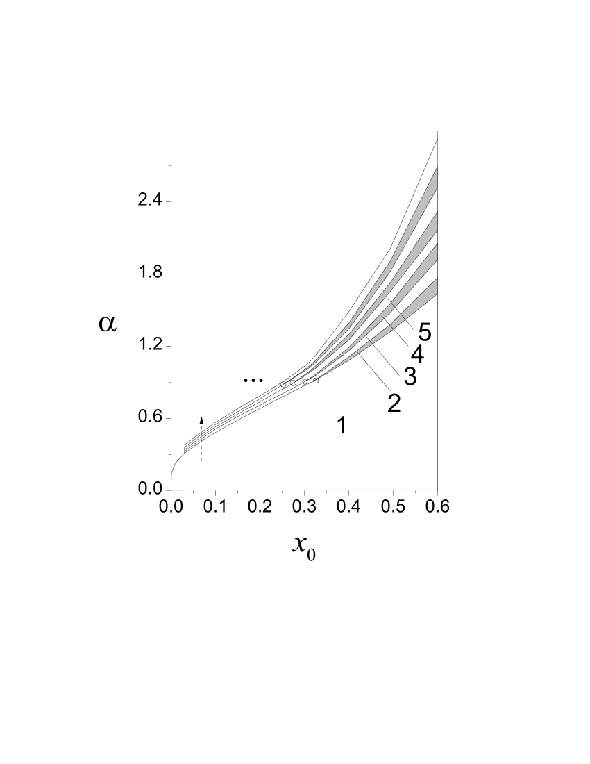
Figure 3: Phase diagram in variables “screening-coupling”. Each phase with certain topology is labeled by the total number of filled and empty regions (see Fig. 1). Even phases (shadowed) are separated from odd ones by “${}^{5}/_{2}$-kind” topological transition (TT) lines, while 2-kind TT lines separate odd phases. Triple points, where two ${}^{5}/_{2}$-TT and one 2-TT meet, are shown by circles. The dashed arrow indicates the phase trajectory studied numerically in Ref. [10].

The energy gain $\Delta\left(\tau\right)$ at TT as a function of small overcriticality parameter $\tau=\alpha/\alpha^{*}-1$ is evidently proportional to $\tau$ times the volume of a new emerging phase region (empty or filled). The analysis shows that the radius of a void (or an island) for a TT with change of parity is $\sim\tau^{1/2}$. Consequently we have $\Delta\left(\tau\right)\sim\tau^{5/2}$ which indicates a similarity of this situation to the known ”${}^{5}/_{2}$-kind” phase transitions in the theory of metals [11], but its specific character is that the new segment of Fermi surface opens at very small momentum values, which can dramatically change the system response to, e.g., electron-phonon interaction. On the other hand, this segment may have a pronounced effect on the thermodynamical properties of ${}^{3}{\textrm{He}}$ at low temperatures, especially in the case of $P$-pairing.

For a TT with unchanged parity, the width of a gap (or a sheet) is found $\sim\tau$, hence the energy gain results $\Delta\left(\tau\right)\sim\tau^{2}$, and such TT can be assigned 2 kind. It follows from the above consideration that each triple point in the $x_{0}-\alpha$ phase diagram is a point of confluence of two ${}^{5}/_{2}$-kind TT lines into one 2-kind line. The latter type of TT was already discussed in literature [9, 10], and we only mention here that its ocurrance on a whole continuous surface in the momentum space is rather specific for systems with strong fermion-fermion interaction, while the known TT’s in metals, under the effects of crystalline field, occur typically at separate points in the quasimomentum space.

It is of interest to note that in the limit $x_{0}\to 0,\alpha\to 0$, reached along a line $\alpha=kx_{0}$, we attain the exactly solvable model: $U(p)\to(2\pi)^{3}U_{0}\delta(p)$ with $U_{0}=k/(2Mp_{{\textrm{F}}})$, which is known to display FC at all $U_{0}>0$ [3]. The analytic mechanism of this behavior consists in that the poles of $U(p)$, eq. (18) tend to zero, thus restoring the analytical properties necessary for FC. Otherwise, the FC regime corresponds to the phase order $\to\infty$, when the density of infinitely thin filled (separated by empty) regions approaches some continuous function $0<\nu(x)<1$ [10] and the dispersion law turns flat by eq. (16).

A few remarks are in order at this point. First, the considered model formally treats $x_{0}$ and $\alpha$ as independent parameters, though in fact a certain relation between them can be imposed. Under such restriction, the system ground state should depend on a single parameter, say the particle density $\rho$, along a certain trajectory $\alpha(x_{0})$ in the above suggested phase diagram. For instance, with the simplest Thomas-Fermi relation for the free electron gas: $\alpha(x_{0})=x_{0}^{2}/2$, this trajectory stays fully within the Fermi state $1$ over all the physically reasonable range of densities. Hence a faster growth of $\alpha(x_{0})$ is necessary for realization of TT in any fermionic system with the interaction, eq. (18).

Second, the single particle potential $V(p)$ of a real system cannot be an entire function of $p$ around $p_{{\textrm{F}}}$ because of the stepwise form of the quasiparticle distribution. Therefore, as the coupling constant moves away from the critical value $\alpha^{*}$ within the WSR domain, the concentric Fermi spheres will be taken up by FC. A close look at the role of the density wave instability, which sets in at sufficiently large $\alpha$, shows that this is true [8]. In fact, these arguments do not work in the case of SSR. Thus, it is quite possible to observe the two separate Fermi sphere regimes. There is a good reason to mention that neither in the case when the FC phase transition takes place nor in the case when types of TT are present the standard Kohn-Sham scheme [14] is no longer valid. Beyond the FC or TT phase transitions the occupations numbers of quasiparticles serve as variational parameters. Thus, to get a reasonable description of the system, one has to consider the ground state energy as a functional of the occupation numbers $E[(n(p)]$ rather then a functional of the density $E[\rho]$ [15]. A more detailed study of such systems, including the finite temperature effects, is in order.

We thank V.A. Khodel and G.E. Volovik for valuable discussions.

This research was supported in part by the Portuguese program PRAXIS XXI through the project 2/2.1/FIS/302/94 and under Grant BPD 14226/97 and in part by the Russian Foundation for Basic Research under Grant 98-02-16170.

References

- [1] L.D. Landau, JETP 30, 1058 (1956).
- [2] J. Bardeen, L. N. Cooper, and J. R. Schrieffer, Phys. Rev. 108, 1175 (1957).
- [3] V.A. Khodel and V.R. Shaginyan, JETP Lett. 51, 553 (1990).
- [4] G.E. Volovik, JETP Lett. 53, 222 (1991).
- [5] P. Nozières, J. Phys. I (Paris) 2, 443 (1992).
- [6] V.A. Khodel, V.R. Shaginyan, and V.V. Khodel, Phys. Rep. 249, 1 (1994).
- [7] D.V. Khveshchenko, R. Hlubina, and T.M. Rice, Phys. Rev. B 48, 10766 (1993).
- [8] V.A. Khodel’, V.R. Shaginyan, and M.V. Zverev, JETP Lett. 65, 253 (1997).
- [9] M. de Llano, J. P. Vary, Phys. Rev. C19, 1083 (1979); M. de Llano, A. Paustino, J.G. Zabolitsky, Phys. Rev. C20, 2418 (1979).
- [10] M.V. Zverev and M. Baldo, cond-mat/9807324, 24 Jul 1998.
- [11] I.M. Lifshitz, Sov. Phys. JETP 11, 1130 (1960).
- [12] We recall that a system with FC also presents a different topological structure (of its Green’s function) from that common for ordinary Fermi liquid, marginal Fermi liquid, and Luttinger liquid [4].
- [13] M. Nakahara, Geometry, topology and physics, IOP Publ., Bristol (1990).
- [14] W. Kohn and L. J. Sham, Phys. Rev. 140, A1133 (1965); see, also, W. Kohn and P. Vashishta, in Theory of the Inhomogeneous Electron Gas, edited by S. Lundqvist and N. H. March (Plenum, New York, 1983); J. Callaway and N. H. March, Solid State Phys. 38, 135 (1983).
- [15] V.R. Shaginyan, JETP Lett. 68, 491 (1998).