Dynamics of Highly Supercooled Liquids

Abstract

The diffusivity of tagged particles is demonstrated to be heterogeneous on time scales comparable to or less than the structural relaxation time in a highly supercooled liquid via 3D molecular dynamics simulation. The particle motions in the relatively active regions dominantly contribute to the mean square displacement, giving rise to a diffusion constant systematically larger than the Stokes-Einstein value. The van Hove self-correlation function $G_{s}(r,t)$ is shown to have a large $r$ tail which can be scaled in terms of $r/t^{1/2}$ for $t\lesssim 3\tau_{\alpha}$, where $\tau_{\alpha}\cong$ the stress relaxation time. Its presence indicates heterogeneous diffusion in the active regions. However, the diffusion process eventually becomes homogeneous on time scales longer than the life time of the heterogeneity structure ($\sim 3\tau_{\alpha}$).

Introduction

Molecular dynamics (MD) simulations can be powerful tools to gain insights into relevant physical processes in highly supercooled liquids. In particular, a number of recent MD simulations have detected dynamic heterogeneities in supercooled model binary mixtures Muranaka ; Harrowell ; Yamamoto_Onuki1 ; Yamamoto_Onuki98 ; yo_prl ; Donati . That is, rearrangements of particle configurations in glassy states are cooperative, involving many molecules, owing to configuration restrictions. Recently, we succeeded in quantitatively characterizing the dynamic heterogeneities in two (2D) and three dimensional (3D) model fluids via MD simulations. We examined bond breakage processes among adjacent particle pairs and found that the broken bonds in an appropriate time interval ($\sim$ the stress relaxation time or the structural $\alpha$ relaxation time $\tau_{\alpha}$) are very analogous to the critical fluctuations in Ising spin systems with their structure factor being excellently fitted to the Ornstein-Zernike form Yamamoto_Onuki1 ; Yamamoto_Onuki98 . The correlation length $\xi$ thus obtained is related to $\tau_{\alpha}$ via the dynamic scaling law, $\tau_{\alpha}\sim\xi^{z}$, with $z=4$ in 2D and $z=2$ in 3D. The heterogeneity structure in the bond breakage is essentially the same as that in jump motions of particles from cages or that in the local diffusivity, as will be discussed below. In this paper, we investigate heterogeneities of tagged particle motions in a 3D supercooled liquid yo_prl .

In a wide range of liquid states, the Stokes-Einstein relation $D\eta a/k_{B}T=const.$ has been successfully applied between the translational diffusion constant $D$ of a tagged particle and the viscosity $\eta$ even when the tagged particle diameter $a$ is of the same order as that of solvent molecules. However, this relation is systematically violated in fragile supercooled liquids Yamamoto_Onuki98 ; yo_prl ; Ediger ; Sillescu ; Ci95 ; Mountain ; Perera_PRL98 . The diffusion process in supercooled liquids is thus not well understood. In particular, Sillescu et al. observed the power law behavior $D\propto\eta^{-\nu}$ with $\nu\cong 0.75$ at low temperatures Sillescu . Furthermore, Ediger et al. found that smaller probe particles exhibit a more pronounced increase of $D\eta/T\propto D/D_{SE}$ with decreasing $T$ Ci95 , where $D_{SE}\sim k_{B}T/2\pi\eta a$ is the Stokes-Einstein diffusion constant. In such experiments the viscosity changes over 12 decades with decreasing $T$, while the ratio $D/D_{SE}$ increases from order 1 up to order $10^{2}\sim 10^{3}$. The same tendency has been detected by molecular dynamics simulations in a 3D binary mixture with $N=500$ particles Mountain and in a 2D binary mixture with $N=1024$ Perera_PRL98 . In our recent 3D simulation with $N=10^{4}$ Yamamoto_Onuki98 ; yo_prl , $\eta$ and $D$ both varied over 4 decades and the power law behavior $D\propto\eta^{-0.75}$ has been observed. Many authors have attributed the origin of the breakdown to heterogeneous coexistence of relatively active and inactive regions, among which the local diffusion constant is expected to vary significantly Sillescu ; Ci95 ; St94 ; Tarjus ; Oppen . The aim of this paper is to demonstrate via MD simulation that the diffusivity of the particles is indeed heterogeneous on time scales shorter than $\tau_{\alpha}$ but becomes homogeneous on time scales much longer than $\tau_{\alpha}$.

Simulation method and results

Our 3D binary mixture is composed of two atomic species, $1$ and $2$, with $N_{1}=N_{2}=5000$ particles with the system linear dimension $L=V^{1/3}$ being fixed at $23.2\sigma_{1}$ Bernu . They interact via the soft-core potentials $v_{ab}(r)=\epsilon(\sigma_{ab}/r)^{12}$ with $\sigma_{ab}=(\sigma_{a}+\sigma_{b})/2$, where $r$ is the distance between two particles and $a,b\in\{1,2\}$. The interaction is truncated at $r=3\sigma_{1}$. The mass ratio is $m_{2}/m_{1}=2$. The size ratio is $\sigma_{2}/\sigma_{1}=1.2$, which is known to prevent crystallization Muranaka ; Bernu . No tendency of phase separation is detected at least in our computation times. We fix the particle density at a very high value of $(N_{1}+N_{2})/V=0.8/\sigma_{1}^{3}$, so the particle configurations are severely restricted or jammed. We will measure space and time in units of $\sigma_{1}$ and $\tau_{0}=({m_{1}\sigma_{1}^{2}/\epsilon})^{1/2}$. The temperature $T$ will be measured in units of $\epsilon/k_{B}$, and the viscosity $\eta$ in units of $\epsilon\tau_{0}/\sigma_{1}^{3}$. The time step $\Delta t=0.005$ is used. In our systems the structural relaxation time becomes very long at low temperatures. Therefore, very long annealing times ($2.5\times 10^{5}$ for $T=0.267$) are chosen in our case. For $T\geq 0.267$, no appreciable aging (slow equilibration) effect is detected in various quantities such as the pressure or the density time correlation function, whereas at $T=0.234$, a small aging effect remains in the density time correlation function.

Figure 1: Coherent and incoherent intermediate scattering functions for various temperatures with $q=2\pi$ (a peak wavenumber in $S_{11}(q,0)$). $T=0.234$, $0.267$, $0.306$, $0.352$, $0.473$, and $0.772$ from right.

Let us first consider the incoherent density correlation function, $F_{s}(q,t)=\langle{\sum_{j=1}^{N_{1}}\exp{[i{\bf q}\cdot\Delta{\mbox{\boldmath$r$}}_{j}(t)]}}\rangle/N_{1}$ for the particle species 1, where $\Delta{\mbox{\boldmath$r$}}_{j}(t)={\mbox{\boldmath$r$}}_{j}(t)-{\mbox{\boldmath$r$}}_{j}(0)$ is the displacement vector of the $j$-th particle. The $\alpha$ relaxation time $\tau_{\alpha}$ is then defined by $F_{s}(q,\tau_{\alpha})=e^{-1}$ at $q=2\pi$ for various $T$. We also calculate the coherent time correlation function, $S_{11}(q,t)=\langle n_{1}({\mbox{\boldmath$q$}},t)n_{1}({-{\mbox{\boldmath$q$}}},0)\rangle$, where $n_{1}({\mbox{\boldmath$q$}},t)=\sum_{j=1}^{N_{1}}\exp{[i{\bf q}\cdot{\mbox{\boldmath$r$}}_{j}(t)]}$ is the Fourier component of the density fluctuations of the particle species 1. The decay profiles of $S_{11}(q,t)$ at its first peak wave number $q=q_{m}\sim 2\pi$ and $F_{s}(q,t)$ at $q=2\pi$ nearly coincide in the whole time region studied ($t<2\times 10^{5}$) within $5\%$ as shown in Fig. 1. Hence $S_{11}(q_{m},\tau_{\alpha})/S_{11}(q_{m},0)\cong e^{-1}$ holds for any $T$ in our simulation. Such agreement is not obtained for other wave numbers, however. These results are consistent with those for a Lennard-Jones binary mixture Kob2 . Furthermore, some neutron-spin-echo experiments Mezei showed that the decay time of $S_{11}(q_{m},t)$ is nearly equal to the stress relaxation time and as a result the viscosity $\eta$ is of order $\tau_{\alpha}$. In agreement with this experimental result, we obtain a simple linear relation in our simulations yo_prl ,

$$\tau_{\alpha}\cong(A_{\eta}/q_{m}^{2})\eta/T.$$ (1)

The coefficient $A_{\eta}$ is close to $2\pi$ in our system. Here, we may define a $q$-dependent relaxation time $\tau_{q}$ by $F(q,\tau_{q})=e^{-1}$. Thus, particularly at the peak wave number $q=q_{m}$, the effective diffusion constant defined by $D_{q}\equiv 1/q^{2}\tau_{q}$ is given by the Stokes-Einstein form even in highly supercooled liquids. However, notice that the usual diffusion constant is the long wavelength limit, $D=\lim_{q\rightarrow 0}D_{q}$. It is usually calculated from the mean square displacement, $\langle{(\Delta{\mbox{\boldmath$r$}}(t))^{2}}\rangle=\langle{\sum_{j=1}^{N_{1}}(\Delta{\mbox{\boldmath$r$}}_{j}(t))^{2}}\rangle/N_{1}.$ The crossover of this quantity from the plateau behavior arising from motions in transient cages to the diffusion behavior $6Dt$ has been found to take place around $t\sim 0.1\tau_{\alpha}$ Yamamoto_Onuki98 . In Fig.2, we plot $D\tau_{\alpha}$ versus $\tau_{\alpha}$, which clearly indicates breakdown of the Stokes-Einstein relation in agreement with the experimental trend.

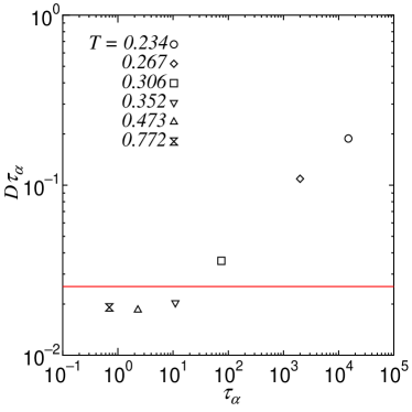
Figure 2: $D\tau_{\alpha}$ versus $\tau_{\alpha}$ in a quiescent supercooled liquid. The solid line represents the Stokes-Einstein value $D_{SE}\tau_{\alpha}=(2\pi)^{-2}$ arising from Eq.(1).

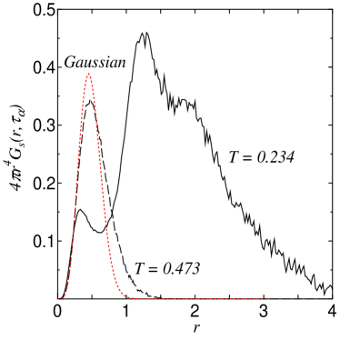
Figure 3: $4\pi r^{4}G_{s}(r,t)$ versus $r$ at $t=\tau_{\alpha}$. The solid line is for $T=0.267$ and the broken line is for $T=0.473$. The dotted line represents the Brownian motion result. The peaks at $r\simeq 1.2$ and $2$ in the solid line arise from hopping processes in our system at $T=0.267$. Note that the areas below the curves give $6D\tau_{\alpha}$.

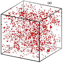
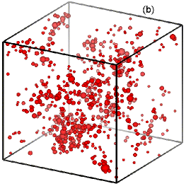
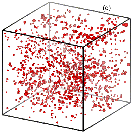
Figure 4: Mobile particles of the species 1 with a time interval $t=\tau_{\alpha}$ at $T=0.473$ (a) and $T=0.267$ (b) and with $t=10\tau_{\alpha}$ at $T=0.267$ (c). The radii of the spheres are $|\Delta{\mbox{\boldmath$r$}}_{j}(t)|/\sqrt{\langle{(\Delta{\mbox{\boldmath$r$}}(t))^{2}}\rangle}$ and the centers are at $\frac{1}{2}[{\mbox{\boldmath$r$}}_{j}(t_{0})+{\mbox{\boldmath$r$}}_{j}(t_{0}+t)]$. The system linear dimension is $L=23.2$. The darkness of the spheres represents the depth in the 3D space.

To examine the diffusion process in more detail, we consider the van Hove self-correlation function, $G_{s}(r,t)=\langle{\sum_{j=1}^{N_{1}}\delta(\Delta{\mbox{\boldmath$r$}}_{j}(t)-{\mbox{\boldmath$r$}})}\rangle/N_{1}.$ Then,

$$F_{s}(q,t)=\int_{0}^{\infty}dr\frac{\sin(qr)}{qr}4\pi r^{2}G_{s}(r,t)$$ (2)

is the 3D Fourier transformation of $G_{s}(r,t)$. At the peak wavenumber $q=2\pi$, the integrand in Eq.(2) vanishes at $r=1$, and the integral in the region $r<1$ is confirmed to dominantly determine the decay of $F_{s}(2\pi,t)$. On the other hand, the mean square displacement

$$\langle{(\Delta{\mbox{\boldmath$r$}}(t))^{2}}\rangle=\int_{0}^{\infty}dr4\pi r^{4}G_{s}(r,t)$$ (3)

is determined by the particle motions out of the cages for $t\gtrsim\tau_{\alpha}$ in glassy states. In Fig.3, we display $4\pi r^{4}G_{s}(r,\tau_{\alpha})$ versus $r$, where $\tau_{\alpha}=3.2$ and $2000$ for $T=0.473$ and $0.267$, respectively. These curves may be compared with the Gaussian (Brownian motion) result, $(2/\pi)^{1/2}\ell^{-3}r^{4}\exp(-r^{2}/2\ell^{2})$, where $3\ell^{2}=6D_{SE}\tau_{\alpha}=3/2\pi^{2}$ is the Stokes-Einstein mean square displacement. Because the areas below the curves give $6D\tau_{\alpha}$, we recognize that the particle motions over large distances $r>1$ are much enhanced at low $T$, leading to the violation of the Stokes-Einstein relation.

We then visualize the heterogeneity of the diffusivity. To this end, we pick up mobile particles of the species 1 with $|\Delta{\mbox{\boldmath$r$}}_{j}(t))|>\ell_{c}$ in a time interval $[t_{0},t_{0}+t]$ and number them as $j=1,\cdots,N_{m}$. Here $\ell_{c}$ is defined such that the sum of $\Delta{\mbox{\boldmath$r$}}_{j}(t)^{2}$ of the mobile particles is $66\%$ of the total sum ($\cong 6DtN_{1}$ for $t\gtrsim 0.1\tau_{\alpha}$). In Fig.4, these particles are drawn as spheres with radii

$$a_{j}(t)\equiv|\Delta{\mbox{\boldmath$r$}}_{j}(t)|/\sqrt{\langle{(\Delta{\mbox{\boldmath$r$}}(t))^{2}}\rangle}$$ (4)

located at ${\mbox{\boldmath$R$}}_{j}(t)\equiv\frac{1}{2}[{\mbox{\boldmath$r$}}_{j}(t_{0})+{\mbox{\boldmath$r$}}_{j}(t_{0}+t)]$ in time intervals $[t_{0},t_{0}+\tau_{\alpha}]$ for $T=0.473$ (a) and $0.267$ (b) and in $[t_{0},t_{0}+10\tau_{\alpha}]$ for $T=0.267$ (c). The the mobile particle number $N_{m}$ is $1595$ in (a), $725$ in (b), and $1316$ in (c), respectively. Here the Gaussian results is $N_{m}=1800$. The ratio of the second moments $c_{2}\equiv\sum_{j=1}^{N_{m}}a_{j}(t)^{2}/\sum_{j=1}^{N_{1}}a_{j}(t)^{2}$ is held fixed at $0.66$, while the ratio of the fourth moments $c_{4}\equiv\sum_{j=1}^{N_{m}}a_{j}(t)^{4}/\sum_{j=1}^{N_{1}}a_{j}(t)^{4}$ turns out to be close to 1 as $c_{4}=0.89$ in (a), $0.92$ in (b), and $0.90$ in (c). The mobile particles are homogeneously distributed for $T=0.473$ at $\tau_{\alpha}$, whereas for $T=0.267$, the heterogeneity is significant at $\tau_{\alpha}$, but is much decreased at $10\tau_{\alpha}$. In fact, the variance defined by ${\cal V}\equiv N_{m}\sum_{j=1}^{N_{m}}a_{j}(t)^{4}/(\sum_{j=1}^{N_{m}}a_{j}(t)^{2})^{2}-1$ is $0.27$ in (a), $0.41$ in (b), and $0.32$ in (c). Note that the statistical average of $\cal V$ (taken over many initial times $t_{0}$) is related to the non-Gaussian parameter $A_{2}\equiv 3\langle{\Delta{\mbox{\boldmath$r$}}(t)^{4}}\rangle/5\langle{\Delta{\mbox{\boldmath$r$}}(t)^{2}}\rangle^{2}-1=3N_{1}\langle{\sum_{j=1}^{N_{1}}a_{j}(t)^{4}}\rangle/5(\langle{\sum_{j=1}^{N_{1}}a_{j}(t)^{2}}\rangle)^{2}-1$ by

$$\langle{{\cal V}}\rangle\cong(5\langle{c_{4}}\rangle\langle{N_{m}}\rangle/3c_{2}^{2}N_{1})(1+A_{2}(t))-1,$$ (5)

where the deviations $c_{4}-\langle{c_{4}}\rangle$ and $N_{m}/\langle{N_{m}}\rangle-1$ are confirmed to be very small for large $N_{1}$ and are thus neglected. We may also conclude that the significant rise of $A_{2}(t)$ in glassy states originates from the heterogeneity in accord with some experimental interpretations Zorn .

We next consider the Fourier component of the diffusivity density defined by

$${\cal D}_{{\mbox{\boldmath$q$}}}(t_{0},t)\equiv\sum_{j=1}^{N_{m}}a_{j}(t)^{2}\exp[-i{\mbox{\boldmath$q$}}\cdot{\mbox{\boldmath$R$}}_{j}(t)],$$ (6)

which depends on the initial time $t_{0}$ and the final time $t_{0}+t$. The correlation function $S_{{\cal D}}(q,t,\tau)=\langle{{\cal D}_{{\mbox{\boldmath$q$}}}(t_{0}+\tau,t){\cal D}_{-{\mbox{\boldmath$q$}}}(t_{0},t)}\rangle$ is then obtained after averaging over many initial states. We plot $S_{{\cal D}}(q,\tau_{\alpha},0)$ in Fig. 5 (a). The heterogeneity structure $S_{b}(q,\tau_{\alpha},0)$ of the bond breakage Yamamoto_Onuki1 ; Yamamoto_Onuki98 with a time interval of $\tau_{\alpha}$ is also plotted in Fig. 5 (b). It is confirmed that $S_{\cal D}(q,\tau_{\alpha},0)$ tends to its long wavelength limit for $q\lesssim\xi^{-1}$, where $\xi$ coincides with the correlation length obtained from $S_{b}(q,\tau_{\alpha},0)$. As the difference $\tau$ of the initial times increases with fixed $t=\tau_{\alpha}$, $S_{{\cal D}}(q,\tau_{\alpha},\tau)$ relaxes as $\exp[-(\tau/\tau_{h})^{c}]$ for $q\lesssim\xi^{-1}$, where $c\sim 0.5$ at $T=0.267$ and $\tau_{h}\sim 3\tau_{\alpha}$ is the life time of the heterogeneity structure. The two-time correlation function among the broken bond density Yamamoto_Onuki1 ; Yamamoto_Onuki98 also relaxes with $\tau_{h}$ in the same manner.

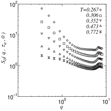
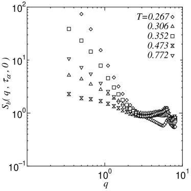
Figure 5: The correlation functions $S_{{\cal D}}(q,\tau_{\alpha},0)$ (a) and $S_{b}(q,\tau_{\alpha},0)$ (b) with $q=2\pi$.

We naturally expect that the distribution of the particle displacement $\Delta{\mbox{\boldmath$r$}}_{j}(t)$ in the active regions should be characterized by the local diffusion constant $D({\mbox{\boldmath$x$}},t)$ dependent on the spatial position ${\mbox{\boldmath$x$}}=(x,y,z)$ and the time interval $t$. The van Hove correlation function $G_{s}(r,t)$ may then be expressed as the spatial average of a local function $G_{s}({\mbox{\boldmath$x$}},r,t)$, which is given by $[4\pi D({\mbox{\boldmath$x$}},t)t]^{-3/2}\exp[-{r^{2}}/4D({\mbox{\boldmath$x$}},t)t]$. To check this conjecture, we plot the scaled function $\sqrt{6Dt}4\pi r^{2}G_{s}(r,t)$ versus $r^{*}=r/\sqrt{6Dt}$ in Fig. 6. The areas below the curves are fixed at 1. At relatively short times $t\lesssim 3\tau_{\alpha}$, the curves in the region $r\gtrsim 1$ or $r^{*}\gtrsim(6Dt)^{-1/2}$, which give dominant contributions to $\langle{(\Delta{\mbox{\boldmath$r$}}(t))^{2}}\rangle$, tend to a master curve quite different from the rapidly decaying Gaussian tail. Note that in each curve the position of the peak at larger $r^{*}$ corresponds to $r\cong 1$. This asymptotic law is consistent with the picture of the space-dependent diffusion constant in the active regions. It is also important that the heterogeneity structure remains unchanged in the time region $t\lesssim\tau_{h}\sim 3\tau_{\alpha}$. At longer times $t\gtrsim 10\tau_{\alpha}$, the curves approach the Gaussian form as can be seen in the inset of Fig.5. Of course, $4\pi r^{2}G_{s}(r,t)$ for $r<1$ does not scale in the above manner, because it is the probability density of a tagged particle staying within a cage. This short-range behavior determines the decay of $F_{s}(2\pi,t)$ as noted below Eq.(2).

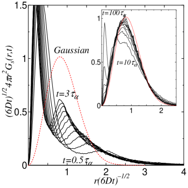
Figure 6: A test of the scaling plot $\sqrt{6Dt}4\pi r^{2}G_{s}(r,t)$ versus $r/\sqrt{6Dt}$ for $0.5\tau_{\alpha}<t<3\tau_{\alpha}$ ($t=(0.5+0.25n)\tau_{\alpha}$, $n=0,1,2,\cdots,10$). The inset shows the curves at longer times, $10\tau_{\alpha}<t<100\tau_{\alpha}$ ($t=10n\tau_{\alpha}$, $n=1,2,\cdots,10$), where the heterogeneity effect is smoothed out. The dotted lines are the Gaussian form.

Concluding remarks

In our previous studies Yamamoto_Onuki1 ; Yamamoto_Onuki98 , we performed extensive MD simulations and identified weakly bonded or relatively active regions from breakage of appropriately defined bonds. We also found that the spatial distributions of such regions resemble the critical fluctuations in Ising spin systems, so the correlation length $\xi$ can be determined. It grows up to the system size as $T$ is lowered, but no divergence seems to exist at nonzero temperatures. In the present work, we have demonstrated that the diffusivity in supercooled liquids is spatially heterogeneous on time scales shorter than $3\tau_{\alpha}$, which leads to the breakdown of the Stokes-Einstein relation yo_prl . The heterogeneity detected is essentially the same as that of the bond breakage in our previous works Yamamoto_Onuki1 ; Yamamoto_Onuki98 . We should then investigate how the heterogeneity arises and influences observable quantities in more realistic glass-forming fluids with complex structures.

References

- (1) Muranaka, T., and Hiwatari, Y., Phys. Rev. E 51, R2735-R2738 (1995); Muranaka, T. and Hiwatari, Y., J. Phys. Soc. Jpn. 67, 1982-1987 (1998).
- (2) Hurley, M.M., and Harrowell, P., Phys. Rev. E 52, 1694-1698 (1995); Perera, D.N., and Harrowell, P., Phys. Rev. E 54, 1652-1662 (1996).
- (3) Yamamoto, R., and Onuki, A., J. Phys. Soc. Jpn. 66, 2545-2548 (1997); Europhys. Lett. 40, 61-66 (1997); Onuki, A., and Yamamoto, R., J. Non-Cryst. Solids 235 -237, 34-40 (1998).
- (4) Yamamoto, R., and Onuki, A. Phys. Rev. E 58, 3515-3529 (1998).
- (5) Yamamoto, R., and Onuki, A., Phys. Rev. Lett. in press (1998).
- (6) Kob, W., et al., Phys. Rev. Lett. 79, 2827-2830 (1997); Donati, C., et al., Phys. Rev. Lett. 80, 2338-2341 (1998).
- (7) Ediger, M.D., Angell, C.A., and Nagel, S.R., J. Phys. Chem. 100, 13200-13212 (1996).
- (8) Fujara, F., Geil, B., Sillescu, H., and Fleischer, G., Z. Phys. B 88, 195-204 (1992); Chang, I., et al., J. Non-Cryst. Solids 172-174, 248-255 (1994).
- (9) Cicerone, M.T., Blackburn, F.R., and Ediger, M.D., Macromolecules 28, 8224-8232 (1995); Cicerone, M.T., and Ediger, M.D., J. Chem. Phys. 104, 7210-7218 (1996).
- (10) Thirumalai, D., and Mountain, R.D., Phys. Rev. E 47, 479-489 (1993).
- (11) Perera, D., and Harrowell, P., Phys. Rev. Lett. 81, 120-123 (1998).
- (12) Stillinger, F.H., and Hodgdon, A., Phys. Rev. E 50, 2064-2068 (1994).
- (13) Tarjus, G., and Kivelson, D., J. Chem. Phys. 103, 3071-3073 (1995).
- (14) Liu, C.Z. -W., and Oppenheim, I., Phys. Rev. E 53, 799-802 (1996).
- (15) Bernu, B., Hiwatari, Y., and Hansen, J.P., J. Phys. C 18, L371-L376 (1985); Bernu, B., Hansen, J.P., Hiwatari, Y., and Pastore, G., Phys. Rev. A 36, 4891-4903 (1987); Matsui, J., Odagaki, T., and Hiwatari, Y., Phys. Rev. Lett. 73, 2452-2455 (1994).
- (16) Kob, W., and Andersen, H.C., Phys. Rev. E 52, 4134-4153 (1995).
- (17) Mezei, F., Knaak, W., and Farago, B., Phys. Rev. Lett. 58, 571-574 (1987); Richter, D., Frick, R., and Farago, B., Phys. Rev. Lett. 61, 2465-2468 (1988).
- (18) Zorn, R., Phys. Rev. B 55, 6249-6259 (1987); Kanaya, T., Tsukushi, I., and Kaji, K., Prog. Theor. Phys. Supplement 126, 133-140 (1997).