Two-Dimensional Quantum Spin Systems with Ladder and Plaquette Structures

1 Introduction

Recent intensive studies on high-$T_{c}$ superconductors and related materials have attracted renewed interest in the quantum phase transitions in low-dimensional spin systems. In particular, a variety of new materials have been found experimentally: For instance, CaV₄O₉ [1, 2, 3], which may be described by the two-dimensional (2D) Heisenberg model on a depleted square lattice, realizes a quantum spin liquid even in two dimension. Also, SrCu₂O₃[4, 5] has been intensively studied as a prototypical example of ladder compounds, [6, 7] for which the introduction of nonmagnetic impurities induces a novel phase transition to the magnetic state. For these materials, the plaquette or ladder structure is essential to stabilize the non-magnetic phase with spin gap. The spin chains with an alternating array of different spins (mixed spin chains or alternating spin chains) also give another new paradigm, [8, 9, 10, 11, 12] for which the topology of spin arrangement plays an essential role to determine the low-energy properties. Quantum phase transitions in the above various low-dimensional spin systems have provided an interesting subject in quantum spin systems.

In our previous paper,[13] by employing non-linear $\sigma$ model (NL$\sigma$M) techniques, we investigated the competition between the gapful and gapless states in a generalized spin ladder which possesses both of the spin and bond alternations. We systematically investigated not only ladder systems but also mixed spin chains and plaquette-type spin chains, and clarified how the competing interactions in addition to topological properties control the quantum phase transitions. In real materials, however, the coupling between ladders or chains neglected in our previous paper becomes certainly important, and may drive the system to the ordered state.

Motivated by the above points, in this paper we study the quantum phase transitions between the ordered and disordered states in 2D spin systems, by extending the previous NL$\sigma$M analysis of the spin chain and ladder systems. In particular, we deal with the 2D antiferromagnetic Heisenberg model with the ladder and plaquette structures, which also possesses the spatial variation of spins (mixed spins). By calculating the spin gap and the spontaneous magnetization by means of NL$\sigma$M and modified spin wave (MSW) approaches, [14, 15] we discuss how the disordered state with spin gap competes against the magnetically ordered state.

The paper is organized as follows. In $\S$2 we introduce a generalized 2D spin model for which both of the bond and spin alternations are included. In $\S$3, by extending the method of Sénéchal,[16] we calculate the spin gap at finite temperatures by means of NL$\sigma$M with saddle-point approximation, and then argue to what extent this approach can describe the quantum phase transitions for 2D systems. We also point out the shortcoming in this approach for spin-$1/2$ systems. In $\S$ 4, we further study the model by using the MSW approach, which qualitatively improves the results of NL$\sigma$M in the spin-$1/2$ case. Brief summary is given in $\S$5.

2 Model Hamiltonian

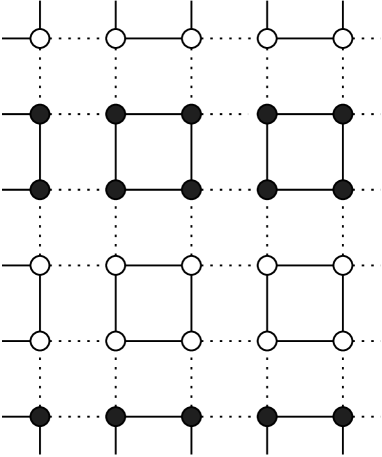
Fig.  1: A generalized 2D spin system with both of the bond and spin alternations.

We introduce a 2D antiferromagnetic spin system with both of the bond and spin alternations, which is described by the following Hamiltonian on a square lattice,

$$H = J_{x}\sum_{i,j}\left[1+(-1)^{i}\gamma_{x}\right]{\mbox{\boldmath$S$}}_{i,j}\cdot{\mbox{\boldmath$S$}}_{i+1,j}$$ (2.1)

$$+ J_{y}\sum_{i,j}\left[1+(-1)^{j}\gamma_{y}\right]{\mbox{\boldmath$S$}}_{i,j}\cdot{\mbox{\boldmath$S$}}_{i,j+1},$$

where $J_{x}$ $(J_{y})$ and $\gamma_{x}$ $(\gamma_{y})$ are the exchange coupling and the bond-alternation parameter along the $x$ $(y)$ direction, respectively. Here ${\mbox{\boldmath$S$}}_{i,j}$ is the spin operator at the $(i,j)$-th site in the $x-y$ plane. Since we deal with the antiferromagnetic case with $J_{x},J_{y}>0$ and $-1\leq\gamma_{x},\gamma_{y}\leq 1$, the ground state of the Hamiltonian (2.1) becomes the Néel state in the classical limit. What is distinct from an ordinary 2D square lattice model is that the present system includes not only the bond alternation but also the spin alternation. For simplicity, we here consider a specific arrangement of two types of spins shown schematically in Fig. 1, where black circles and white circles denote the spins $s_{1}$ and $s_{2}$. The generalized Hamiltonian (2.1) allows us to study a variety of interesting spin systems which possess a ladder structure, a plaquette structure, and a mixture of different spins. This is a natural extension of our previous analysis of the mixed-spin chains and ladders [13] to more realistic cases including the effects of two dimensionality. In the next section we shall first study the model by employing the NL$\sigma$M techniques.

3 Non-Linear Sigma Model Analysis

In this section we discuss the competition between the spin-gapped phase and the magnetically ordered phase by taking the non-linear $\sigma$ model (NL$\sigma$M) as a low energy effective theory. Let us begin by briefly summarizing how NL$\sigma$M techniques are applied to our model in the continuum limit. Using the coherent-state path integral formalism,[17] the partition function in the present system is given by

$$Z=\int{\rm D}\mbox{\boldmath$\Omega$}_{ij}\exp\left[-{\rm i}\sum_{ij}s_{ij}\omega\left[\mbox{\boldmath$\Omega$}_{ij}\right]-\int_{0}^{\beta}{\rm d}\tau H\left(\tau\right)\right],$$

(3.1)

where

$$\omega\left[{\mbox{\boldmath$\Omega$}}_{ij}\right] = \int_{0}^{\beta}{\rm d}\tau\dot{\varphi}_{ij}(1-\cos\theta_{ij}),$$ (3.2)

$$H(\tau) = J_{x}\sum_{i,j}s_{i,j}s_{i+1,j}\left[1+(-1)^{i}\gamma_{x}\right]{\mbox{\boldmath$\Omega$}}_{i,j}\cdot{\mbox{\boldmath$\Omega$}}_{i+1,j}$$

$$+ J_{y}\sum_{i,j}s_{i,j}s_{i,j+1}\left[1+(-1)^{j}\gamma_{y}\right]{\mbox{\boldmath$\Omega$}}_{i,j}\cdot{\mbox{\boldmath$\Omega$}}_{i,j+1}.$$

In the above expressions we have introduced the unit vector $\Omega$ by ${\mbox{\boldmath$S$}}=s{\mbox{\boldmath$\Omega$}}$, where ${\mbox{\boldmath$\Omega$}}=(\sin\theta\cos\varphi,\sin\theta\sin\varphi,\cos\theta)$. The term $\omega\left[{\mbox{\boldmath$\Omega$}}\right]$ is the Berry phase. In the present approach we assume that the usual spin-wave analysis can correctly describe low-energy modes at wave vectors near $(0,0),(0,\pi),(\pi,0)$, and $(\pi,\pi)$. The last one corresponds to the ordering wave vector. Then the unit vector ${\mbox{\boldmath$\Omega$}}_{i,j}$ can be written in terms of three fluctuation fields and one staggered field as follows[16]

$$\mbox{\boldmath$\Omega$}_{2i+\alpha,2j+\beta}=(-1)^{\alpha+\beta}\mbox{\boldmath$n$}\left(\mbox{\boldmath$r$}^{\prime}\right),$$ (3.4)

$$\mbox{\boldmath$n$}\left(\mbox{\boldmath$r$}^{\prime}\right)=\phi\left(\mbox{\boldmath$r$}\right)+a{\sum_{mn}}^{{}^{\prime}}(-1)^{m\alpha+n\beta}\mbox{\boldmath$l$}_{mn}^{(k)}\left(\mbox{\boldmath$r$}\right),$$ (3.5)

where $\mbox{\boldmath$r$}^{\prime}=\mbox{\boldmath$r$}+\alpha m+\beta n$, $m(n)$ and $\alpha(\beta)$ runs from $0$ to $1$, and $a$ is the lattice constant. The primed sum means that the term $m=n=0$ is omitted. Therefore fluctuations which we take here are $l_{01}$, $l_{10}$, and $l_{11}$ for each site. The point we wish to notice is that the fluctuation $l$ is further distinguished by the index $k(=1,2)$, corresponding to spins $s_{1}$ and $s_{2}$, respectively. The staggered field $\phi$ is a slowly varying field on the scale of the lattice spacing. Substituting eq.(3.4) into eq.(LABEL:eqn:Htau) and making the expansion up to quadratic order in $\mbox{\boldmath$l$},\mbox{\boldmath$\phi$}^{\prime}$, and $\dot{\mbox{\boldmath$\phi$}}$, we arrive at the following Hamiltonian in the continuum limit

$$H\left(\tau\right) = \int{\rm d}\mbox{\boldmath$r$}\left(h_{x}+h_{y}\right),$$ (3.6)

$$h_{x} = \frac{J_{x}}{2}\left[\left(s_{1}^{2}+s_{2}^{2}\right)\left(1+\gamma_{x}\right)\left(\partial_{x}\mbox{\boldmath$\phi$}\right)^{2}\right.$$ (3.7)

$$+2\left(1+\gamma_{x}\right)\partial_{x}\mbox{\boldmath$\phi$}\cdot\left(s_{1}^{2}\mbox{\boldmath$l$}_{10}^{(1)}+s_{2}^{2}\mbox{\boldmath$l$}_{10}^{(2)}\right)$$

$$+2\sum_{j}\left.\left(s_{1}^{2}{\mbox{\boldmath$l$}_{1j}^{(1)}}^{2}+s_{2}^{2}{\mbox{\boldmath$l$}_{1j}^{(2)}}^{2}\right)\right],$$

$$h_{y} = \frac{J_{y}}{4}\left[2\left(1-\gamma_{y}\right)\sum_{i}\left(s_{1}^{2}{\mbox{\boldmath$l$}_{i1}^{(1)}}^{2}+s_{2}^{2}{\mbox{\boldmath$l$}_{i1}^{(2)}}^{2}\right)\right.$$ (3.8)

$$+4s_{1}s_{2}\left(1+\gamma_{y}\right)\left[\left(\partial_{y}\mbox{\boldmath$\phi$}\right)^{2}+\partial_{y}\mbox{\boldmath$\phi$}\cdot\left(\mbox{\boldmath$l$}_{01}^{(1)}+\mbox{\boldmath$l$}_{01}^{(2)}\right)\right]$$

$$\left.+s_{1}s_{2}\left(1+\gamma_{y}\right)\sum_{i}\left(\mbox{\boldmath$l$}_{i1}^{(1)}+\mbox{\boldmath$l$}_{i1}^{(2)}\right)^{2}\right].$$

The Berry phase in this system is given by

$$S_{\rm Berry} = {\rm i}\sum_{ij}s_{ij}\omega\left[\mbox{\boldmath$\Omega$}_{ij}\right]$$ (3.9)

$$= \frac{\rm i}{2a}\int{\rm d}\mbox{\boldmath$r$}\left(s_{1}\mbox{\boldmath$l$}_{11}^{(1)}+s_{2}\mbox{\boldmath$l$}_{11}^{(2)}\right)\cdot\mbox{\boldmath$\phi$}\times\dot{\mbox{\boldmath$\phi$}}.$$

Integrating eq. (3.1) over the fluctuation fields $l$, we thus end up with the NL$\sigma$M

$$Z = \int{\rm D}{\mbox{\boldmath$\phi$}}\exp\left\{-\frac{1}{2g}\left[\frac{1}{v}\left(\partial_{\tau}{\mbox{\boldmath$\phi$}}\right)^{2}\right.\right.$$ (3.10)

$$\left.\left.+vR_{x}\left(\partial_{x}{\mbox{\boldmath$\phi$}}\right)^{2}+vR_{y}\left(\partial_{y}{\mbox{\boldmath$\phi$}}\right)^{2}\right]\right\}.$$

Note that the Berry phase terms cancel out in the present system and do not show up in the effective action. This simple result allows us to further investigate the quantum phase transitions by employing ordinary NL$\sigma$M techniques. Since general forms of parameters $g,v,R_{x}$, and $R_{y}$ are rather complicated, we shall show their concrete formulae for each case discussed in the following.

3.1 Gap equation

To proceed the calculation based on the NL$\sigma$M, further approximations may be needed. Here we use the saddle point approximation to obtain the spin gap equation from eq.(3.10), by extending the treatment of Sénéchal.[16] The validity of this approximation will be discussed later in this section. In what follows, we set the speed $v=1$; it can be restored by dimensional analysis at the end of the calculation. Rescaling the field $\mbox{\boldmath$\phi$}\rightarrow\sqrt{g}\mbox{\boldmath$\phi$}$, the Lagrangian (3.10) is now written as

$$L = \frac{1}{2}\left[\left(\partial_{\tau}{\mbox{\boldmath$\phi$}}\right)^{2}+R_{x}\left(\partial_{x}{\mbox{\boldmath$\phi$}}\right)^{2}+R_{y}\left(\partial_{y}{\mbox{\boldmath$\phi$}}\right)^{2}\right.$$ (3.11)

$$\left.-\sigma\left({\mbox{\boldmath$\phi$}}^{2}-1/g\right)\right],$$

where $\sigma$ is the Lagrange multiplier to enforce the constraint $\mbox{\boldmath$\phi$}^{2}=1/g$. Integrating eq.(3.11) over the field $\phi$, we obtain the effective potential to the field $\sigma$

$$V(\sigma) = \frac{\sigma}{2g}-\frac{1}{\beta}\sum_{\omega_{n}}\int\frac{{\rm d}\mbox{\boldmath$k$}}{(2\pi)^{2}}$$ (3.12)

$$\times\log\left(1+\frac{\sigma}{\omega_{n}^{2}+R_{x}k_{x}^{2}+R_{y}k_{y}^{2}}\right).$$

Here we replace the field $\sigma$ by the uniform value, which corresponds to the square of the spin gap. To evaluate the spin gap, the magnon speed $v$ is restored by dimensional analysis. Finding out the saddle point of the potential eq.(3.12), we obtain the spin gap equation

$$\frac{1}{g}=\int \frac{{\rm d}\mbox{\boldmath$k$}}{(2\pi)^{2}}\frac{1}{\sqrt{R_{x}k_{x}^{2}+R_{y}k_{y}^{2}+(\Delta/v)^{2}}}$$ (3.13)

$$\times\coth\frac{\beta}{2}\sqrt{R_{x}k_{x}^{2}+R_{y}k_{y}^{2}+(\Delta/v)^{2}}.$$

It is to be noticed that a momentum cut-off parameter $\Lambda$, which is proportional to the inverse lattice spacing $a^{-1}$, should be introduced in the above expression. Since it is hard to determine the cut-off procedure only from the present theory, we use other means to fix it. We outline a procedure for the case of plaquette structure characterized by the parameters: $\gamma=\gamma_{x}=\gamma_{y},J=J_{x}=J_{y}$. In the limit $\gamma\rightarrow 1$ the system changes to the assembly of plaquette singlets. Then the spin gap of the system is exactly $\Delta=2J$ at $T=0$. Requiring that the gap obtained from eq.(3.13) with $\gamma=1$ should be equal to $2J$, the cut-off parameter is chosen as $a\Lambda=\sqrt{2\pi/3}$. Assuming that this value can be used for other values of $\gamma$, we discuss the low-energy properties of spin systems with plaquette structure.

This completes our formulation of the model in terms of NL$\sigma$M approach. In the following we show the numerical results obtained for the 2D spin systems with plaquette and ladder structures, as well as the mixed spin system.

3.2 Plaquette-structure system

Let us start our discussions for the spin system with plaquette structure with the parameters, $\gamma=\gamma_{x}=\gamma_{y},J=J_{x}=J_{y}$, for which spins are assumed to be uniform ($s=s_{1}=s_{2}$). In this case, the parameters in NL$\sigma$M are given by

$$\begin{array}[]{rcl}R_{x}&=&\left(1-\gamma_{x}^{2}\right)j,\\ R_{y}&=&1-\gamma_{y}^{2},\\ g&=&2a\sqrt{1+j}/s,\\ v&=&2J_{y}sa\sqrt{1+j},\end{array}$$ (3.14)

where $j$ is defined by $j=J_{x}/J_{y}$. The cut-off parameter, as already mentioned, is taken as $a\Lambda=\sqrt{2\pi/3}$.

Fig.  2: Normalized spin gap $\delta(=\Delta/\Delta_{0})$ for spin $s=1/2$ (a) and $s=1$ (b) plaquette structures calculated by the NL$\sigma$M. It is shown as a function $t(=aT)$. $\Delta_{0}$ is the spin gap at $T=0$.

The behavior of the normalized spin gap $\delta(=\Delta/\Delta_{0})$ is shown as a function of the temperature $t(=aT)$ for spin $s=1/2$ (Figs. 2(a)) and $s=1$ (Figs. 2(b)) systems. $\Delta_{0}$ is the spin gap at $T=0$. Physically, the spin gap should be regarded as the inverse of the correlation length. As the temperature is decreased, the spin gap (inverse correlation length) decreases, and reaches zero or a finite value according to the nature of ground state. For the $s=1$ case, we can clearly observe the quantum phase transition at $T=0$ in Fig. 2(b) when we decrease the value of $\gamma$ from unity. At $\gamma=1$, the system at $T=0$ is composed of isolated plaquettes and forms the plaquette singlet ground state which possesses the spin gap in the excitation. In decreasing $\gamma$, the plaquette-singlet state with spin gap is driven to the magnetically ordered state, which is realized for $\gamma\leq\gamma_{c}$. As is the case for ordinary 2D quantum systems with continuous symmetry, the ordered state is allowed only for $T=0$, which is correctly described in our treatment, as is seen from the figure. Although the NL$\sigma$M approach has produced qualitatively correct results for the case with $s>1/2$, we can not find the quantum phase transition to the ordered state for $s=1/2$, as seen from Fig. 2 (a). This is contradicted to the well-known fact that the ground state of the $s=1/2$ isotropic square lattice ($\gamma=0$) should be an antiferromagnetically ordered state. This implies that our approach may not sufficiently take into account antiferromagnetic fluctuations, and this shortcoming may come mainly from the saddle point approximation we used. In order to improve our results for the $s=1/2$ case, we further study the system by employing modified spin wave approach in the next section.

3.3 Ladder-structure system

Next we investigate the 2D system with ladder structure which is realized by choosing $\gamma_{x}=0$ and $\gamma=\gamma_{y}$. This is the system composed of periodic array of ladders along $y$-direction.[18] By appropriately tuning the interaction strength, we can naturally interpolate from the isolated ladders to the 2D system with ladder structure. The corresponding couplings for NL$\sigma$M is given by the same expression as (3.14).

Fig.  3: Normalized spin gap $\delta(=\Delta/\Delta_{0})$ for the spin $s=1/2$ (a) and $s=1$ (b) ladder systems calculated by the NL$\sigma$M ($j=1/2)$. It is shown as a function $t(=aT)$.

The cut-off parameter in the ladder system is taken as $a\Lambda=0.99$, which is determined according to the numerical results[19, 20] ($\Delta/J=0.504$) for the uniform isotropic ladder ($j=1/2$). The results for the spin gap are shown in Figs. 3 for the cases of $s=1/2$ and $1$. Note that the system with the parameter $\gamma=0(1)$ corresponds to the isotropic square lattice (the isolated ladder). For the isolated ladder, the system should have the spin gap, which is consistent with our results. By decreasing $\gamma$ from unity, we observe the quantum phase transition at $T=0$ from the spin-gapped phase to the magnetic phase for $s=1$, but not for $s=1/2$. As is the case for the model with plaquette structure, we thus describe the quantum phase transition properly for $s>1/2$. The problem we have encountered again for $s=1/2$ has the same origin mentioned before for the plaquette case. We shall come to this problem in the next section.

3.4 Mixed spin system

So far, we have considered the uniform-spin systems. We note that mixed spin chains with periodic array of several kind of different spins have also attracted much attention both experimentally and theoretically. [8, 9, 10, 11] For example, mixed spin chains with either the ferrimagnetic ground state or the singlet ground state have been intensively studied. [9, 10, 11] In the previous paper,[13] we have studied the mixed spin chains by NL$\sigma$M approach. To make the theoretical model more realistic, it may be natural to take into account the coupling among mixed chains. We address this problem in this section. As a simple example of mixed spin systems, we here consider the spin system composed of two different spins $s_{1}=1$ and $s_{2}=3/2$ (and also $s_{1}=1/2$ and $s_{2}=1$) for the 2D system shown in Fig. 1. This type of system enables us to bridge 2D quantum systems and mixed spin chains mentioned above. To make our discussions simpler, we deal with the system without bond alternation. Then parameters in NL$\sigma$M for the mixed spin system are given by

$$R_{x} = \frac{j}{8}\frac{\left(1+\alpha\right)^{2}\left(1+\alpha^{2}\right)}{\alpha^{2}},$$ (3.15)

$$R_{y} = 1,$$ (3.16)

$$g = \frac{1+\alpha}{s_{2}}aK,$$ (3.17)

$$v = \frac{4J_{y}s_{2}a}{1+\alpha}K,$$ (3.18)

where $K=\sqrt{(2j+1)[(1+\alpha)^{2}+4j\alpha]/[(1+\alpha)^{2}+8j\alpha]}$ and $\alpha=s_{2}/s_{1}$.

Fig.  4: Normalized spin gap $\delta(=\Delta/\Delta_{0})$ for the mixed spin system, for $s_{1}=1$, $s_{2}=3/2$, calculated by the NL$\sigma$M. It is shown as a function $j(=J_{x}/J_{y})$.

The cut-off parameter is taken as $a\Lambda=1.41$ according to the numerical results in ref[21]: $\Delta/J=0.41\;(T=0,s_{1}=s_{2}=1,j=0)$. The normalized spin gap calculated for $s_{1}=1$ and $s_{2}=3/2$ is shown in Fig. 4. For $j=0$, the system is composed of isolated mixed spin chains, which is known to be massive, being consistent with the present results.[13] When the value of $j$ is increased, the system gradually changes to the 2D system. We then find a plausible result that there exists the critical value of $j$ at which the system is changed to the ordered state. For the $s_{1}=1/2$ and $s_{2}=1$ case , however, we have checked that in the whole range of $j$ the system has the spin gap, and the long range order does not show up. Since we naturally expect that for moderately large $j$ the antiferromagnetic ground state may be stabilized, we should improve our treatment for this case, which is reexamined in the next section by MSW approach.

4 Modified Spin-Wave Approach

We have so far studied our 2D spin model by the NL$\sigma$M with saddle point approximation, by employing the method of Sénéchal [16], which is a natural extension of our previous study on the spin chain and spin ladder systems.[13] Although qualitative features for the quantum phase transitions have been described for the systems with larger spins, we have encountered the problem for the $s=1/2$ cases as well as the mixed spin case with $s=1/2,1$, for which our NL$\sigma$M analysis may not describe the correct phase transition. We think that this shortcoming comes mainly ¿from our saddle point approximation, which may not properly incorporate magnetic correlations for $s=1/2$ case. To improve this point, there may be several possible ways. The one is to apply renormalization-group analysis to the NL$\sigma$M instead of saddle point approximation, which was successfully applied to 2D $s=1/2$ systems. [22] Alternatively, there exists a different but similar approach based on the modified spin wave (MSW) approximation.[14, 15] This method is known to provide rather satisfactory results for the isotropic $s=1/2$ spin systems, which are comparable to the renormalization group method mentioned above. For instance, both of the above methods have produced the correct temperature dependence of the correlation length for the 2D $s=1/2$ spin systems on square lattice. Therefore, the MSW approach is expected to provide a sensible rout to improve our results for small $s$ cases in the previous section. In what follows, we treat the present model within the MSW approximation. We show the formulation in the case of uniform spins, for simplicity, since it is straightforward to extend it to the system composed of two distinct spins.

By the Holstein-Primakoff transformation, the spin operators are expressed in terms of boson creation and annihilation operators as follows

$$\begin{array}[]{ll}\begin{array}[]{l}S_{\mbox{\sevenmib r}}^{z}=s-a_{\mbox{\sevenmib r}}^{{\dagger}}a_{\mbox{\sevenmib r}}\\ S_{\mbox{\sevenmib r}}^{+}=\sqrt{2s-a_{\mbox{\sevenmib r}}^{{\dagger}}a_{\mbox{\sevenmib r}}}\;\;a_{\mbox{\sevenmib r}}\end{array}&{\mbox{\boldmath$r$}}=(2i,2j)\in A,\\ \begin{array}[]{l}S_{\mbox{\sevenmib r}}^{z}=b_{\mbox{\sevenmib r}}^{{\dagger}}b_{\mbox{\sevenmib r}}-s\\ S_{\mbox{\sevenmib r}}^{+}=b_{\mbox{\sevenmib r}}^{{\dagger}}\sqrt{2s-b_{\mbox{\sevenmib r}}^{{\dagger}}b_{\mbox{\sevenmib r}}}\end{array}&{\mbox{\boldmath$r$}}=(2i+1,2j)\in B,\\ \begin{array}[]{l}S_{\mbox{\sevenmib r}}^{z}=c_{\mbox{\sevenmib r}}^{{\dagger}}c_{\mbox{\sevenmib r}}-s\\ S_{\mbox{\sevenmib r}}^{+}=c_{\mbox{\sevenmib r}}^{{\dagger}}\sqrt{2s-c_{\mbox{\sevenmib r}}^{{\dagger}}c_{\mbox{\sevenmib r}}}\end{array}&{\mbox{\boldmath$r$}}=(2i,2j+1)\in C,\\ \begin{array}[]{l}S_{\mbox{\sevenmib r}}^{z}=s-d_{\mbox{\sevenmib r}}^{{\dagger}}d_{\mbox{\sevenmib r}}\\ S_{\mbox{\sevenmib r}}^{+}=\sqrt{2s-d_{\mbox{\sevenmib r}}^{{\dagger}}d_{\mbox{\sevenmib r}}}\;\;d_{\mbox{\sevenmib r}}\end{array}&{\mbox{\boldmath$r$}}=(2i+1,2j+1)\in D.\\ \end{array}$$ (4.1)

Boson operators $a_{\mbox{\sevenmib r}},b_{\mbox{\sevenmib r}},c_{\mbox{\sevenmib r}},d_{\mbox{\sevenmib r}}$ belong to the A, B, C, D sublattices, respectively. Since the unit cell in our system includes four sites, we have introduced four kinds of Bose operators. In case that we consider the system with two kinds of spins, eight kinds of bosons should be introduced. The Fourier transformations are defined as

$$\alpha_{\mbox{\sevenmib r}}=\sqrt{\frac{4}{N}}\sum_{\mbox{\sevenmib k}}\alpha_{\mbox{\sevenmib k}}e^{-{\rm i}{\mbox{\sevenmib k}}\cdot{\mbox{\sevenmib r}}} \beta_{\mbox{\sevenmib r}}=\sqrt{\frac{4}{N}}\sum_{\mbox{\sevenmib k}}\beta_{\mbox{\sevenmib k}}e^{{\rm i}{\mbox{\sevenmib k}}\cdot{\mbox{\sevenmib r}}},$$ , (4.2)

for $\alpha=a,d(\beta=b,c)$, where $N$ is the total number of lattice, and the summation over momenta $k$ is restricted to the quarter of the original Brillouin zone. Then Hamiltonian becomes

$$H = 2J_{y}s\sum_{\mbox{\sevenmib k}}\left\{(1+j)\left(a_{\mbox{\sevenmib k}}^{{\dagger}}a_{\mbox{\sevenmib k}}+b_{\mbox{\sevenmib k}}^{{\dagger}}b_{\mbox{\sevenmib k}}+c_{\mbox{\sevenmib k}}^{{\dagger}}c_{\mbox{\sevenmib k}}+d_{\mbox{\sevenmib k}}^{{\dagger}}d_{\mbox{\sevenmib k}}\right)\right.$$ (4.3)

$$+j\kappa_{x}\left[\left(a_{\mbox{\sevenmib k}}b_{\mbox{\sevenmib k}}+c_{\mbox{\sevenmib k}}^{{\dagger}}d_{\mbox{\sevenmib k}}^{{\dagger}}\right)e^{{\rm i}\phi_{x}}+{\rm H.c.}\right]$$

$$\left.+\kappa_{y}\left[\left(a_{\mbox{\sevenmib k}}c_{\mbox{\sevenmib k}}+b_{\mbox{\sevenmib k}}^{{\dagger}}d_{\mbox{\sevenmib k}}^{{\dagger}}\right)e^{{\rm i}\phi_{y}}+{\rm H.c.}\right]\right\},$$

where

$$\kappa_{x} = \sqrt{1-(1-\gamma_{x}^{2})\sin^{2}k_{x}},$$

$$\phi_{x} = \arg\left[\cos k_{x}+{\rm i}\gamma_{x}\sin k_{x}\right],$$

$$\kappa_{y} = \sqrt{1-(1-\gamma_{y}^{2})\sin^{2}k_{y}},$$

$$\phi_{y} = \arg\left[\cos k_{y}+{\rm i}\gamma_{y}\sin k_{y}\right].$$

The diagonalization of the Hamiltonian (4.3) yields the conventional spin wave excitations. The staggered magnetization per site is expressed as

$$m = \frac{1}{N}\left[\sum_{{\mbox{\sevenmib r}}\in A}S_{\mbox{\sevenmib r}}^{z}-\sum_{{\mbox{\sevenmib r}}\in B}S_{\mbox{\sevenmib r}}^{z}-\sum_{{\mbox{\sevenmib r}}\in C}S_{\mbox{\sevenmib r}}^{z}+\sum_{{\mbox{\sevenmib r}}\in D}S_{\mbox{\sevenmib r}}^{z}\right]$$ (4.4)

$$= s-\frac{1}{N}\sum_{\mbox{\sevenmib k}}\left[a_{\mbox{\sevenmib k}}^{{\dagger}}a_{\mbox{\sevenmib k}}+b_{\mbox{\sevenmib k}}^{{\dagger}}b_{\mbox{\sevenmib k}}+c_{\mbox{\sevenmib k}}^{{\dagger}}c_{\mbox{\sevenmib k}}+d_{\mbox{\sevenmib k}}^{{\dagger}}d_{\mbox{\sevenmib k}}\right].$$

Here it should be noticed that the sublattice symmetry [15] in the ground state is broken. In order to extend our study into the region of the disordered phase, we restore this symmetry by enforcing the following constraint on eq.(4.3),

$$s=\frac{1}{N}\sum_{\mbox{\sevenmib k}}\left[a_{\mbox{\sevenmib k}}^{{\dagger}}a_{\mbox{\sevenmib k}}+b_{\mbox{\sevenmib k}}^{{\dagger}}b_{\mbox{\sevenmib k}}+c_{\mbox{\sevenmib k}}^{{\dagger}}c_{\mbox{\sevenmib k}}+d_{\mbox{\sevenmib k}}^{{\dagger}}d_{\mbox{\sevenmib k}}\right].$$ (4.5)

This means that the staggered magnetization (4.4) should be zero in the disordered phase. Since the constraint may give rise to the spin gap in a certain parameter region, we can discuss the phase transition ¿from the ordered phase to the disordered phase with spin gap. Using the Lagrange multiplier $\lambda$, the Hamiltonian with the constraint (4.5) is cast to

$$H^{{}^{\prime}}=H-\lambda\sum_{\mbox{\sevenmib k}}\left[a_{\mbox{\sevenmib k}}^{{\dagger}}a_{\mbox{\sevenmib k}}+b_{\mbox{\sevenmib k}}^{{\dagger}}b_{\mbox{\sevenmib k}}+c_{\mbox{\sevenmib k}}^{{\dagger}}c_{\mbox{\sevenmib k}}+d_{\mbox{\sevenmib k}}^{{\dagger}}d_{\mbox{\sevenmib k}}\right].$$ (4.6)

By the Bogoliubov transformations

$$\left(\begin{array}[]{c}a_{\mbox{\sevenmib k}}\\ b_{\mbox{\sevenmib k}}^{{\dagger}}\\ c_{\mbox{\sevenmib k}}^{{\dagger}}\\ d_{\mbox{\sevenmib k}}\end{array}\right)=\frac{1}{\sqrt{2}}\left(\begin{array}[]{cc}U_{\mbox{\sevenmib k}}^{+}&U_{\mbox{\sevenmib k}}^{-}\\ V_{\mbox{\sevenmib k}}^{+}&V_{\mbox{\sevenmib k}}^{-}\end{array}\right)\left(\begin{array}[]{l}\alpha_{\mbox{\sevenmib k}}^{(1)}\\ \alpha_{\mbox{\sevenmib k}}^{(2){\dagger}}\\ \beta_{\mbox{\sevenmib k}}^{(1)}\\ \beta_{\mbox{\sevenmib k}}^{(2){\dagger}}\end{array}\right),$$ (4.7)

where

$$U_{\mbox{\sevenmib k}}^{\pm}=\mp e^{-{\rm i}\phi_{y}}\left(\begin{array}[]{cc}-\cosh\theta_{\mbox{\sevenmib k}}^{\pm}&\sinh\theta_{\mbox{\sevenmib k}}^{\pm}e^{-{\rm i}\phi_{x}}\\ \sinh\theta_{\mbox{\sevenmib k}}^{\pm}e^{{\rm i}\phi_{x}}&-\cosh\theta_{\mbox{\sevenmib k}}^{\pm}\end{array}\right)$$ (4.8)

$$V_{\mbox{\sevenmib k}}^{\pm}=\left(\begin{array}[]{cc}-\sinh\theta_{\mbox{\sevenmib k}}^{\pm}&\cosh\theta_{\mbox{\sevenmib k}}^{\pm}e^{-{\rm i}\phi_{x}}\\ \cosh\theta_{\mbox{\sevenmib k}}^{\pm}e^{{\rm i}\phi_{x}}&-\sinh\theta_{\mbox{\sevenmib k}}^{\pm}\end{array}\right)$$ (4.9)

$$\cosh\theta_{\mbox{\sevenmib k}}^{\pm} = \frac{1}{\sqrt{2}}\sqrt{\frac{1}{\epsilon_{\mbox{\sevenmib k}}^{\pm}}+1},$$ (4.10)

$$\epsilon_{\mbox{\sevenmib k}}^{\pm} = \sqrt{1-\frac{1}{\mu^{2}}\left(\frac{j\kappa_{x}\pm\kappa_{y}}{1+j}\right)^{2}},$$ (4.11)

$$\mu = 1-\frac{\lambda}{2(J_{x}+J_{y})s},$$ (4.12)

the Hamiltonian (4.6) is diagonalized as

$$H=\sum_{\mbox{\sevenmib k}}\sum_{i=1}^{2}\left[E_{\mbox{\sevenmib k}}^{+}\alpha_{\mbox{\sevenmib k}}^{(i){\dagger}}\alpha_{\mbox{\sevenmib k}}^{(i)}+E_{\mbox{\sevenmib k}}^{-}\beta_{\mbox{\sevenmib k}}^{(i){\dagger}}\beta_{\mbox{\sevenmib k}}^{(i)}\right].$$ (4.13)

where the energy dispersion $E_{\mbox{\sevenmib k}}^{\pm}$ is defined by $2(J_{x}+J_{y})s\mu\epsilon_{\mbox{\sevenmib k}}^{\pm}$. The spin gap $\Delta$ opens at $\mbox{\boldmath$k$}=(0,0)$, and is estimated as

$$\Delta=\sqrt{\lambda^{2}-4(J_{x}+J_{y})s\lambda}.$$ (4.14)

We can easily confirm that in the case of $\lambda=0$ this theory is identical with the conventional spin-wave theory and that the lowest mode of the system has the linear dispersion.

In order to formulate thermodynamics, we introduce the probability, $P_{i\mbox{\sevenmib k}}^{+}(n_{i}^{+})$ ($P_{i\mbox{\sevenmib k}}^{-}(n_{i}^{-})$), for the state with the wave vector $k$ being occupied by $n_{i}^{+}$($n_{i}^{-}$) bosons with type $\alpha^{(i)}$($\beta^{(i)}$). Then the free energy has the form

$$F = \sum_{\mbox{\sevenmib k},i,n}\left\{E_{\mbox{\sevenmib k}}^{+}nP_{i\mbox{\sevenmib k}}^{+}(n)+E_{\mbox{\sevenmib k}}^{-}nP_{i\mbox{\sevenmib k}}^{-}(n)\right.$$ (4.15)

$$- \left.\left[\mu_{i\mbox{\sevenmib k}}^{+}P_{i\mbox{\sevenmib k}}^{+}(n)+\mu_{i\mbox{\sevenmib k}}^{-}P_{i\mbox{\sevenmib k}}^{-}(n)\right]\right\}-TS,$$

where $\mu_{i\mbox{\sevenmib k}}^{\pm}$ is the generalized chemical potential, and $S$ is the entropy. By evaluating $P_{i\mbox{\sevenmib k}}^{\pm}(n)$ which minimizes the free energy $F$, we end up with an ordinary formula,

$$P_{i\mbox{\sevenmib k}}^{\pm} = \left(1-\exp\left[-E_{\mbox{\sevenmib k}}^{\pm}/T\right]\right)\exp\left[-nE_{\mbox{\sevenmib k}}^{\pm}/T\right].$$ (4.16)

Taking the $N\rightarrow\infty$, the resulting constraint has the form

$$s+\frac{1}{2}=\frac{1}{\pi^{2}}\int_{0}^{\frac{\pi}{2}}{\rm d}k_{x}\int_{0}^{\frac{\pi}{2}}{\rm d}k_{y}\left[\frac{1}{\epsilon_{\mbox{\sevenmib k}}^{+}}\coth\frac{E_{\mbox{\sevenmib k}}^{+}}{2T}+\frac{1}{\epsilon_{\mbox{\sevenmib k}}^{-}}\coth\frac{E_{\mbox{\sevenmib k}}^{-}}{2T}\right].$$

(4.17)

This completes the MSW formulation of our model. Solving the above equation to determine the chemical potential $\lambda$, we then evaluate the spin gap at finite temperatures from eq.(4.14).

In the following we discuss the results separately for three cases studied in the previous section.

4.1 Plaquette-structure system

Let us first show the results obtained for the system with plaquette structure. We here focus on the $s=1/2$ system for which our NL$\sigma$M approach with saddle-point approximation has encountered the problem.

Fig.  5: Spin gap $\Delta$ for the plaquette structure calculated within the MSW approximation. It is shown as a function of the temperature$T$.

Fig.  6: Staggered magnetization $m$ (the dashed line) and the spin gap $\Delta$ (the solid line) for the plaquette structure calculated within the MSW approximation.

The present MSW approach provides us with not only the temperature dependence of the spin gap (Fig. 5) but also the staggered magnetization at $T=0$ (Fig. 6). We find in Fig. 5 that, in contrast with the results of the NL$\sigma$M, the solid line for $\gamma=0$ reproduces the gapless behavior at $T=0$. Moreover we can see in Fig. 6 that when $\gamma=0$, the system has a finite magnetization ($m=0.303$). The magnetization decreases with increasing $\gamma$ and finally vanishes at the critical value $\gamma_{c}=0.798$. For $\gamma\geq\gamma_{c}$ the plaquette-singlet ground state with spin gap is stabilized, as mentioned in the previous section. These results qualitatively improve the results of NL$\sigma$M with saddle-point approximation since the effect of antiferromagnetic correlation may be treated more properly in the MSW approximation. Though the MSW can qualitatively describe the correct behavior of the quantum phase transition, it may be plausible to evaluate various quantities more quantitatively. To this end, we have also performed a complementary calculation based on the cluster expansion starting from the isolated spin plaquette, up to fourth order, which has been developed by several groups recently.[23] By applying the Padé approximation to the above series expansion, we have confirmed that there indeed exists the quantum phase transition and the critical value $\gamma_{c}$ is around 0.3.[24] This largely improves the result of the MSW quantitatively. The detail for the results of the cluster expansion will be reported elsewhere.

4.2 Ladder-structure system

We next consider the 2D $s=1/2$ system with ladder structure discussed in the previous section.[18] In Fig. 7, the spin gap calculated by the MSW is shown as a function of the temperature for several choices of the bond alternation parameter.

Fig.  7: Spin gap $\Delta$ in the $s=1/2$ ladder structure for $j=2$ calculated by the MSW approximation.

It is seen from Fig. 7 that there is a critical strength of the bond-alternation parameter $\gamma_{c}$ at which the correlation length (inverse of the spin gap) becomes large with decreasing temperature, and diverges at zero temperature. For $\gamma<\gamma_{c}$, the spontaneous antiferromagnetic order emerges, but only at zero temperature. In Fig. 8, we show the phase diagram in terms of the bond alternation parameter $\gamma$ and the anisotropic parameter $j=J_{x}/J_{y}$. If we fix $\gamma$ to be an appropriate value, the quantum phase transitions may be observed twice with the increase of $j$. If $j$ is very small, the system is approximated by weekly coupled spin chains with dimerization. This phase is massive because of the dimer gap for the spin chain. When $j$ is increased, the system is driven to the 2D antiferromagnetically ordered state. If $j$ is further increased, the system may be described by a weakly coupled ladder system which should be again massive, and thus we encounter the second phase transition.

Fig.  8: Phase diagram of the ladder system calculated by the MSW approximation (see the results of ref.[18]). The broken line is the phase boundary determined by the dimer expansion method up to fifth order combined with the Padé approximants. We have also shown the results of the Quantum Monte Carlo calculation[18] by the dots.

We should note here that the present ladder-structure system at $T=0$ was previously studied by Katoh and Imada by MSW theory.[18] Our results at $T=0$ indeed coincide with their results. Furthermore, they have performed the Monte Carlo calculations, and confirmed the quantum phase transition at the critical strength of the bond-alternation parameter, and estimated its value rather precisely, which improves the results of the MSW quantitatively. In this connection, we have also performed the calculation based on the dimer expansion[23] up to fifth order by taking isolated dimers for rungs as a starting point. This approach may be complementary to the Monte Carlo approach of Katoh and Imada. The phase boundary determined by the dimer expansion method with Padé approximation is plotted in Fig. 8 with broken line for smaller $j$ region, which shows fairly good agreement with Monte Carlo results.

4.3 Mixed spin system

As mentioned in the previous section, the mixed spin chains have attracted much current interest. Although we could describe the quantum phase transition for the $s=1,3/2$ mixed system qualitatively by NL$\sigma$M approach, we failed to do for the $s=1/2,1$ mixed case, which may be most interesting from the viewpoint of experiments. We address the latter case in this subsection. In Fig. 9, we show the results for the spin gap and spontaneous magnetization calculated by MSW method for mixed spin system with $s=1/2,1$.

Fig.  9: The staggered magnetization $m$ (the dashed line) and the spin gap $\Delta$ (the solid line) for the $s=1/2,1$ mixed spin system calculated by the MSW approximation. The calculated quantities are shown as a function $j(=J_{x}/J_{y})$.

For $j=0$, the system is reduced to the mixed spin chain with the periodic array of spins as $\cdots 11\frac{1}{2}\frac{1}{2}11\frac{1}{2}\frac{1}{2}\cdots$, so that it is in the massive phase because of the topological nature of the system.[13] This is consistent with the results of NL$\sigma$M. In contrast to NL$\sigma$M approach, however, the spin gap rapidly decreases in the vicinity of $j=0$, and the systems is driven to the ordered phase with a finite staggered magnetization at $j_{c}=0.009$.

Up to now, the mixed spin chains found experimentally are known to exhibit the ferrimagnetic ground state.[8] It may be expected that the mixed spin chains with singlet ground state, as discussed here, may be also fabricated experimentally in the future. Then such mixed spin chains should provide an interesting paradigm of quantum spin systems, for which the topological nature of spatial variation of spins control the low-energy properties of the systems. In particular, it may be interesting to observe how such massive systems are driven to the magnetically ordered phase in the presence of the interchain coupling, impurities, etc.

5 Summary

By extending our previous studies on the spin chain and ladders, we have systematically investigated quantum phase transitions in 2D spin systems with plaquette and ladder structures. In these systems, the lattice structure as well as the competing interactions play a crucial role to determine low-energy properties. By computing the spin gap and the spontaneous magnetization, by NL$\sigma$M and MSW approaches, we have confirmed that both of the above approaches describe the quantum phase transition qualitatively well, so far as the system with larger spins is concerned. However, it has turned out that for $s=1/2$ systems (as well as $s=1/2,1$ mixed spin systems), the NL$\sigma$M with saddle point approximation cannot properly describe the phase transition. So, this approach employed recently by Sénéchal may not be appropriate to discuss the phase transition even at qualitative level for $s=1/2$ spin models. On the other hand, the MSW treatment, which may be provide the results comparable to the renormalization group treatment of NL$\sigma$M, has been shown to plausibly describe the phase transition for $s=1/2$.

In order to give more quantitative discussions for the quantum phase transitions, we have also shown some preliminary calculations based on the series expansion methods such as the dimer expansion, the plaquette expansion, etc, which indeed improve the results of NL$\sigma$M and MSW. To derive more precise information on these quantum spin systems, it is desirable to extend the cluster expansion to higher orders systematically, which is now under consideration.

6 Acknowledgements

The work is partly supported by a Grant-in-Aid ¿from the Ministry of Education, Science, Sports, and Culture.

References

- [1] S. Taniguchi, T. Nishikawa, Y. Yasui, Y. Kobayashi, M. Sato, T. Nishioka, M. Kontani, and K. Sano: J. Phys. Soc. Jpn. 64 (1995) 2758.
- [2] K. Ueda, H. Kontani, M. Sigrist, and P. A. Lee: Phys. Rev. Lett. 76 (1996) 1932.
- [3] O. A. Starykh, M .E. Zhitomirsky, D. I. Khomskii, R. R. P. Singh, and K. Ueda: Phys. Rev. Lett. 77 (1996) 2558.
- [4] Z. Hiroi, M. Azuma, M. Yakano, and I. Bando: J. Solid State Chem. 95 (1991) 230
- [5] For a review, E. Dagotto and T. M. Rice: Science 271 (1996) 618.
- [6] M. Azuma, Y. Fujishiro, M. Takano, T. Ishida, K. Okuda, M. Nohara and H. Takagi: Phys. Rev. B55 (1997) R8658.
- [7] H. Fukuyama, N. Nagaosa, M. Saito and T. Tanimoto: J. Phys. Soc. Jpn. 65 (1996) 2377; Y. Motone, N. Katoh, N. Furukawa and M. Imada: J. Phys. Soc. Jpn. 65 (1996) 1949; M. Sigrist and A. Furusaki: J. Phys. Soc. Jpn. 65 (1996) 2385; N. Nagaosa, A. Furusaki, M. Sigrist and H. Fukuyama: J. Phys. Soc. Jpn. 65 (1996) 3724; Y. Iino and M. Imada: J. Phys. Soc. Jpn. 65 (1996) 3728.
- [8] G. T. Yee, J. M. Manriquez, D. A Dixon, R. S. McLean, D. M. Groski, R. B. Flippen, K. S. Narayan, A. J. Epstein and J. S. Miller: Adv. Mater. 3 (1991) 309; Inorg. Chem. 22 (1983) 2624; ibid. 26 (1987) 138.
- [9] S. K. Pati, S. Ramasesha and D. Sen: Phys. Rev. B55 (1997) 8894; A. K. Kolezhuk, H.-J. Mikeska and S. Yamamoto, ibid. 55 (1997) 3336; F. C. Alcaraz and A. L. Malvezzi: J. Phys. A30 (1997) 767; H. Niggemann, G. Uimin and J. Zittartz: J. Phys. Cond. Matt.: 9 (1997) 9031.
- [10] H. J. de Vega and F. Woynarovich: J. Phys. A25 (1992) 449; M. Fujii, S. Fujimoto and N. Kawakami: J. Phys. Soc. Jpn. 65 (1996) 2381.
- [11] T. Tonegawa, T. Hikihara, T. Nishino, M. Kaburagi, S. Miyashita and H.-J. Mikeska: J. Phys. Soc. Jpn. 67 (1998) 1000.
- [12] T. Fukui and N. Kawakami: Phys. Rev. B55 (1997) R14712; Phys. Rev. B56 (1997) 8799.
- [13] A. Koga, S. Kumada, N. Kawakami, and T. Fukui: J. Phys. Soc. Jpn. 67 (1998) 622.
- [14] M. Takahashi: Phys. Rev. B40 (1989) 2494.
- [15] J. E. Hirsch and S. Tang: Phys. Rev. B40 (1989) 4769.
- [16] D. Sénéchal: Phys. Rev. B47 (1993) 8353; D. Sénéchal: Phys. Rev. B48 (1993) 15880.
- [17] For standard text books, E. Fradkin: Field Theories of Condensed Matter Physics (Addison-Weslay Publishing, Redwood City, 1994); A. M. Tsvelik: Quantum Field Theory in Condensed Matter Physics (Cambridge University Press, New York, 1995).
- [18] N. Katoh and M. Imada: J. Phys. Soc. Jpn 63 (1994) 4529.
- [19] E. Dagotto, J. Riera, and D. J. Scalapino: Phys. Rev. B45 (1992) 5744.
- [20] S. R. White, R. M. Noack and D. J. Scalapino: Phys. Rev. Lett. 73 (1994) 886.
- [21] M. P. Nightingale and H. W. Blöte: Phys. Rev. B33 (1986) 659.
- [22] S. Chakravarty, B. I. Halperin and D. R. Nelson: Phys. Rev. B39 (1989) 2344.
- [23] R. R. P. Singh, M. P. Gelfand, and D. A. Huse: Phys. Rev. Lett. 61 (1988) 2484; H. X. He, C. J. Hamer, and J. Oitmaa: J. Phys. A 23 (1990) 1775; K. Hida: J. Phys. Soc. Jpn. 61 (1992) 1013.
- [24] Recently similar results have been reported by Y. Fukumoto and A. Oguchi: J. Phys. Soc. Jpn. 67 (1998) 2205.