Interface pinning and slow ordering kinetics on infinitely ramified fractal structures.
Abstract
We investigate the time dependent Ginzburg-Landau (TDGL) equation for a non conserved order parameter on an infinitely ramified (deterministic) fractal lattice employing two alternative methods: the auxiliary field approach and a numerical method of integration of the equations of evolution. In the first case the domain size evolves with time as , where is the anomalous random walk exponent associated with the fractal and differs from the normal value , which characterizes all Euclidean lattices. Such a power law growth is identical to the one observed in the study of the spherical model on the same lattice, but fails to describe the asymptotic behavior of the numerical solutions of the TDGL equation for a scalar order parameter. In fact, the simulations performed on a two dimensional Sierpinski Carpet indicate that, after an initial stage dominated by a curvature reduction mechanism à la Allen-Cahn, the system enters in a regime where the domain walls between competing phases are pinned by lattice defects. The lack of translational invariance determines a rough free energy landscape, the existence of many metastable minima and the suppression of the marginally stable modes, which in translationally invariant systems lead to power law growth and self similar patterns. On fractal structures as the temperature vanishes the evolution is frozen, since only thermally activated processes can sustain the growth of pinned domains.
PACS numbers: 64.60C, 64.60M, 64.60A
introduction
The study of the relaxation dynamics of a system initially in thermal equilibrium and abruptly rendered unstable by a sudden change of a controlling field has recently drawn considerable attention, not only because many physical properties may depend on the way a material reaches the equilibrium state, but also because it poses intriguing problems to the theory such as broken ergodicity, aging and dynamical scaling [1],
After the quench, i.e. a rapid lowering of the temperature below the critical point of a phase separating system, the initial, disordered state looses stability and the system undergoes a coarsening process, during which the domains corresponding to different equilibrium phases compete to grow in magnitude. About twenty years ago, Allen and Cahn [2] realized that when the order parameter is non conserved, the driving force towards equilibrium stems from the tendency of the system to reduce the curvature of the domain walls and showed that the typical size of the domains , , increases in time with a power law behavior . In spite of the fact that the theory of phase ordering in homogeneous systems is pretty well understood, only recently the ordering kinetics on non-translationally invariant, fractal lattices, has become a subject of investigation.
The present author in collaboration with Petri [3]- [4] considered the role of deterministic fractal supports, with finite and infinite order of ramification, on the ordering process employing the so-called spherical model, which has the advantage of rendering analytical approaches possible. It was found by means of an explicit solution that the spherical model on fractal lattices of finite order of ramification, such as the Sierpinski gasket of arbitrary embedding dimension does not display a finite temperature phase transition; on the contrary on Sierpinski Carpets, whose order of ramification is infinite [5]-[6], there exist an order-disorder transition provided that the spectral dimension exceeds the critical value [7], in accord with the Mermin-Wagner theorem [8].
Interestingly, the study of the spherical model with non conserved order parameter has revealed the existence, even on fractals, of a characteristic length scale , which increases in time in a power like fashion , and of dynamical scaling for the correlation functions. Such a dynamical exponent takes the value on Sierpinski gaskets of arbitrary embedding dimension , and on the planar Sierpinski Carpet, where is the random walk exponent. These values of differ from the Allen-Cahn universal value , which characterizes the diffusive domain growth on standard lattices. We have shown [3] that in order to fully characterize the static and dynamical properties of the spherical model on fractal lattices two more quantities are required: i) the fractal dimension and ii) the spectral dimension , which for many lattices are related to via the Alexander-Orbach [9] relation:
Unfortunately the analytically soluble spherical model does not yield predictions which can be extrapolated to the physically interesting case of the scalar order parameter. In fact, the lack of sharp, well defined interfaces between different phases, renders the spherical model physically inadequate to describe the phase separation process of an Ising system.
The purpose of the present paper is to investigate the phase separation process on fractals with infinite ramification order, such as the Sierpinski Carpet family , for a non conserved scalar order parameter. We expect the latter to be very sensitive to the presence of inhomogeneities in contrast with vector fields. The choice of a Sierpinski Carpet has been suggested by the fact that it represents perhaps the simplest example of non stochastic fractal lattice, with infinite ramification order [5], [10]. In section II we introduce the Ginzburg-Landau (GL) model on the fractal lattice, in III we consider an auxiliary field approach [11] and discuss its asymptotic behavior. In IV we present numerical results of the exact equations of motion and monitor in several ways the growth process. In V after stressing the similarities between the auxiliary field method and the spherical model, we draw the conclusions.
I Ginzburg-Landau model on a fractal lattice.
We shall consider a scalar field whose properties depend on a standard Ginzburg-Landau free energy functional and defined at every lattice cell, whose coordinate we represent by :
| (1) |
where and are the quadratic and quartic couplings of the GL theory while the first term is proportional to the surface energy. We shall focus on the dynamical properties of the GL model on the two dimensional deterministic Sierpinski Carpet (SC), of fractal dimension (Hausdorff dimension) .
In order to construct the SC, one divides a square lattice of cells, with , into blocks of equal size and the cells contained in the central block are discarded. Dividing again each of the remaining blocks into sub-blocks and discarding all the central elements as many times as necessary to have the smallest sub-blocks constituted of a single cell, one obtains a structure of cells, where .
We make the assumption that the evolution towards equilibrium of the order parameter, , at the site is given by the Ginzburg-Landau equation:
| (2) |
Here represents a Gaussian white noise with zero average and variance :
where is the temperature of the final equilibrium state, is a kinetic coefficient and the Kronecker symbol.
By substituting eq. (1) into (2) we find that , at any time after the quench, changes according to the equation:
| (3) |
We shall write as a difference operator in analogy with the discrete representation of the Laplacian on Euclidean lattices. Periodic boundary condition are assumed, unless explicitly stated. The operator is defined as:
where counts the number of nearest neighbors of the site .
At temperature , the free energy has two two equivalent minima . In the case of the spherical model we showed that the critical temperature vanishes when the spectral dimension is less than , while in the scalar case the critical temperature of a Sierpinski Carpet is finite [12]. In the following, we shall concentrate on the dynamical properties for deep quenches .
II auxiliary field approach
In this section the so called auxiliary field method [1], [11] and [13], which has provided new insight into the ordering dynamics of translationally invariant systems, will be applied to the non conserved order parameter dynamics on the Sierpinski Carpet.
In this approach one replaces the physical field by an auxiliary field, , which varies in a smoother fashion across the interfaces and renders approximations feasible.
One chooses a non linear transformation from to a new field in such a way that the latter obeys to an equation simpler than the original one. If such equation is linear, the statistical properties of are equivalent to those of free gaussian fields and analytical work can be performed. Following the presentation of De Siena and Zannetti [11], one way of determining the transformation is to require that the auxiliary field linearizes the local part of the original equation of evolution (i.e. a zero dimensional version of eq. (3), obtained by setting ). For convenience, unless stated explicitly we shall assume the stiffness constant and the kinetic coefficient to be 1. The auxiliary field is introduced via the mapping:
| (4) |
In order to obtain the equation of motion for the auxiliary field, , we need to consider the non local term:
| (5) |
where the sum is restricted to the nearest neighbors of the site . Assuming that is a slowing varying function of , one can expand the field at a nearest neighbor site in a Taylor series:
| (6) |
having indicated with primes the derivatives of with respect to and neglected higher order terms (H.O.T.) in the expansion. Collecting together the terms from the nearest neighbors one obtains:
| (7) |
The equation of motion for the auxiliary field reads:
| (8) |
To obtain eq. (8) we have used the identities:
| (9) |
and
| (10) |
To proceed further, we consider a mean-field like approximation for the last term in eq.(8):
| (11) |
Introducing the abbreviation:
| (12) |
the equation of evolution for the auxiliary field reads:
| (13) |
Upon neglecting the last term in eq. (13), i.e. setting , we recover the Kawasaki, Yalabik and Gunton (KYG) theory [14]. Alternatively, we expand the function to first order in the coupling constant and write [11]:
| (14) |
The field thus evolves according to an equation similar to the one found in the spherical model and in the Hartree-like approximation, the non linear term being treated self-consistently.
In order to obtain the properties of the field we consider the eigenvalue problem:
| (15) |
where is the -th component of the eigenvector associated with the eigenvalue of the operator . There is an eigenvalue associated with the uniform mode whose eigenvector has all elements equal. The asymptotic behavior of the solution of eq. (14) depends on the distribution of the smallest eigenvalues. After expanding the field as a linear superposition of modes of amplitude :
| (16) |
one finds that each component evolves independently as:
| (17) |
The quantity must be calculated self-consistently from the governing equation (14):
| (18) |
where the average is over the initial conditions of the field . Using eq. (12) and the eigenfunction expansion of we compute as:
| (19) |
For a continuum density of states approximation is appropriate and one can write:
| (20) |
where is proportional to the amplitude of the fluctuations of the field at the instant . One ends with a closed equation for :
| (21) |
From eq. (21) one sees that the quantity must behave as
| (22) |
Thus asymptotically the quantity goes to a constant value , while the equal-time correlation function diverges as:
| (23) |
It is possible, now, to compute the correlation function:
| (24) |
A scaling form for the above quantity is (see [15]):
| (25) |
where is the distance between the sites and . The above correlation function yields the following average value for the droplet size, , as a function of time:
| (26) |
Knowing the evolution of the field it is possible to determine the properties of the original field . Recalling that has a Gaussian distribution at all times, one writes:
| (27) |
where represents a normalization factor:
| (28) |
with
| (29) |
and
| (30) |
| (31) |
The average value of the original field can be calculated from:
| (32) |
while its correlator is given by:
| (33) |
Using the form of the distribution function and eq.(33) one finds for the correlation function of the field the result (see [13]):
| (34) |
Substituting eqs.(23),(25) and (31) into eq. (34) one obtains:
| (35) |
which predicts a smooth decay of the correlation at long distances and the existence of dynamical scaling behavior in the late stage growth.
To check the above results we have solved the equations of evolution (14) numerically on a Sierpinski Carpet of size and monitored the growth by measuring the fluctuation of the homogeneous component of the order parameter:
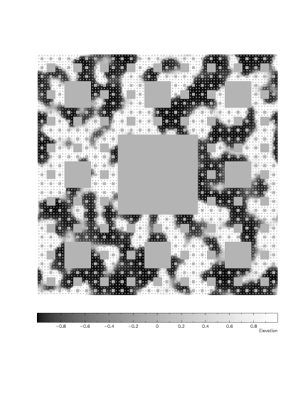
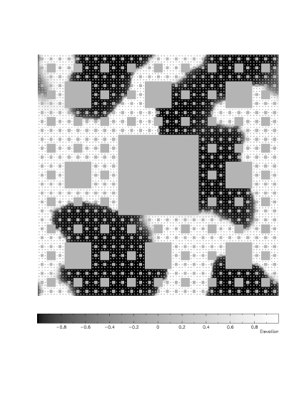
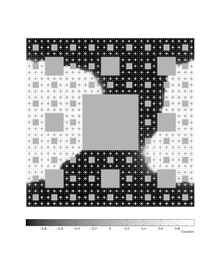
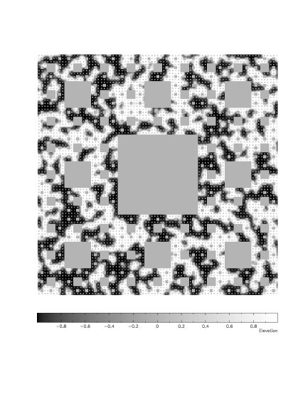
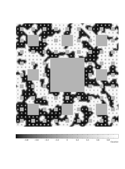
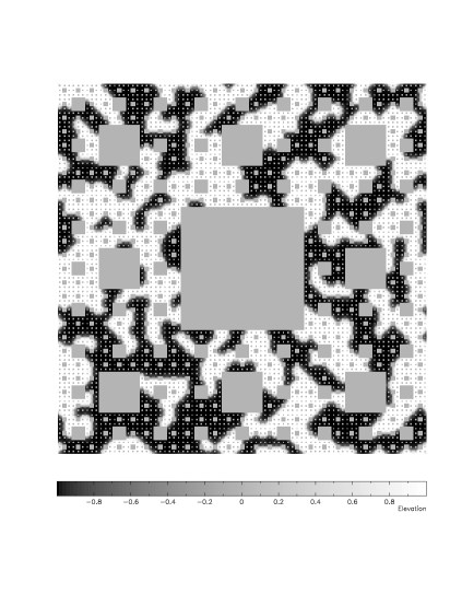
which is the zero component of the structure factor and grows in time, as shown in fig. (1), with an apparent exponent in agreement with the spherical model result [4] which gives , with . The morphology of the field obtained inserting the solution into the non linear mapping eq. (4) is shown in figs.(2-4) and reveals the existence of large droplets growing in time in a fashion similar to that observed on compact supports, as if the fractality affects only the mass-to-size ratio of the domains, but does not suppress the diffusive motion of the walls. In this sense the auxiliary field method agrees quite well with the behavior of the spherical model.
In the next section we shall compare these findings with a direct simulation of the Langevin equation.
III Numerical results
We have investigated numerically the non conserved dynamics on the Sierpinski Carpet starting from a disordered state, generated assigning to each cell a random number uniformly distributed in the interval and assumed . In order to integrate numerically eq. (8) we adopted an Euler discretization scheme with time step and Sierpinski Carpets of different linear sizes with periodic boundary conditions. We have checked that our results do not change appreciably if we decrease further . We also considered several temperatures quenches and runs up to . The averages for the various quantities presented below refer to 50 independent random initial configurations. In order to measure the droplet size we have applied the Hoshen-Kopelman algorithm [16] to label the individual clusters formed by nearest neighbor cells characterized by the same sign of the order parameter. Quantitative measures of the droplet properties are their masses and the radii of gyration. The mass, , is defined as the number of cell belonging to a droplet, while the radius of gyration is defined as:
The sum is over the lattice sites belonging to a droplet, is the position of the lattice sites and the position of its center of mass. To compute the mean value of as a function of time we averaged over all droplets and over all initial configurations.
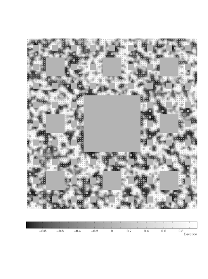
The growth law for the average size of the droplets is reported in fig.(5) and the data are compared with those referring to an Euclidean square lattice of the same linear size. We observe that the growth is much slower in the first system than in the second. In figs. (6-8) are shown typical snapshots of the system: the domain walls, separating opposite phases, sit on locations where the surface energy cost is lower and thermal fluctuations are needed to push the system out of these minima. Further evidence of the absence of power-law growth stems from the study of , which is compared in fig. (9) with the corresponding quantity in the Euclidean case, known to grow as .
Since in the late stage the characteristic width of the interfaces does not change appreciably with time, another independent measure of the domain structure is given by the ratio between the total number of sites and the number of sites covered by interfaces, the so called inverse perimeter density [17]:
By assigning a perimeter site every time the absolute value of was less than the value , one obtains an estimate of which is not too sensitive to the above threshold. While displays power law growth in translationally invariant structures and grows proportionally to , in the fractal case saturates at a constant value for low temperature quenches as shown in fig.(10).
Another quantity with good self-averaging properties is the surface energy density (fig.(11)), whose time dependence we studied and compared with the Euclidean case. For compact supports this quantity decays as the inverse of the domain size , while on the Carpet it displays slow relaxation and eventually freezes.
Based on these results one is lead to the conclusion that, after the early regime, the average domain size and other indicators do not grow with a power law behavior, as found in Euclidean lattices and in the spherical model on the same fractal support. At zero temperature one finds a breakdown of the self-similar dynamical scaling, in contrast with the compact case. Notice that the crossover from a diffusive and curvature driven dynamics to a thermally activated, Arrhenius-like, dynamics is not disorder induced as in the case of Ising diluted models [18]-[21]. During the early stage the domains coarsen almost linearly with time because the curvature provides the main driving mechanism, while at later times the growth becomes much slower and eventually stops since the height of the barriers that the domain walls have to surmount increases with the domain size. The dynamics selects configurations, in which regions of opposite magnetization are separated by boundaries formed by a large number of voids. Since these configurations are associated with low surface tension the interfaces remain trapped.
Interestingly, the crossover time from a power law growth regime, during which the trapping is not effective, to a frozen state is independent of the value of the stiffness constant . This is understood by recalling that during the early stage the domain size grows diffusively as:
The pinning typically occurs when a moving interface encounters voids of size of the order of the interfacial width , which scales as . Recalling that the distance between two voids of linear dimension is proportional to itself, (due to the deterministic nature of the fractal) the typical separation of two domain walls is proportional to . The asymptotic radius of the droplets is:
which gives a crossover time :
Therefore the interfacial stiffness, determines the typical size of the droplets, but not the crossover time scale at which the freezing occurs.
Asymmetric, off-critical quenches lead to immediate equilibration of one of the two phases, and fragmented patterns are not observed. On the other hand, when one considers the conserved order parameter dynamics on percolation structures [24] even off-critical quenches fail to generate the ordered state during a cooling at reasonable rate and lead to frozen dynamic behavior with interrupted growth at low temperatures.
Twisted boundary conditions.
We finally looked at the effect on the phase ordering dynamics of a lattice with twisted boundary conditions along the x-direction of the lattice, maintaining the periodicity along the y-direction . As the compact system orders and forms two large domains of the opposite equilibrium phases, separated by rather sharp interfaces. On the contrary, on a fractal the system remains frozen in a highly fragmented structure as shown in fig.(12) because of the presence of voids, which reduce the role of the curvature. To characterize the interfacial roughness we consider the following correlator:
where represents the width of the system and the two arguments denote the longitudinal and transverse coordinate respectively. In the case of the regular lattice, the peak of narrows as the interface becomes straighter and sharper, while in the case of the fractal remains multi-peaked, as the interface pervades all the volume as illustrated in fig. (13). One can go further by defining a characteristic width of the interface as:
As the time saturates to a much larger value than the corresponding quantity in a Euclidean lattice with identical boundary conditions and random initial conditions.
IV Discussion and conclusions
On regular lattices, domain walls on sufficiently large scales can be approximated in the continuum limit by smooth curved interfaces, which either grow or shrink, whereas in the fractal case the background lattice has a pronounced influence on the phase separation. In a translationally invariant system the origin of the power law like behavior can be traced back to the interfacial motion: immediately after the temperature quench, the system relaxes rapidly along the directions with the steepest gradients of the free energy and the order parameter sets locally to one its equilibrium values , leaving the system disordered, due to the presence of multiple domains of opposite phases separated by thin walls. This early regime is followed by a slower dynamics during which the driving force stems from the movement of the domain walls in order to reduce the interfacial energy . In other words, a curved portion of an interface will move and its velocity will be proportional to its local curvature, while a planar portion in the absence of thermal fluctuations comes at rest. The slow behavior of the late stage reflects the flatness of the energy landscape. One can think of the representative point of the system as moving along a direction characterized by a very small gradient of the free energy .
Let us consider the free energy Hessian :
its eigenvalue spectrum gives a measure of the stability of a selected configuration and reveals the origin of the slow directions of relaxation. If at a given time the configuration is close to one of the global minima of , i.e.. those characterized by uniform values of the field , the spectrum contains only positive eigenvalues and the resulting relaxation process is an exponential function of time. On the other hand, a symmetric quench leads almost inevitably to the formation of a domain structure, which is associated to a saddle point and not to a minimum in phase space [22]. Thus the Hessian calculated in correspondence of the droplet solution must have a negative eigenvalue which corresponds to the expanding mode. The approach to equilibrium consists of the passage from the unstable droplet configuration to one of the absolute minima. Since the droplet size increases in time the free energy becomes flatter and flatter along the unstable path and the instability is reduced. Correspondingly the associated negative eigenvalue vanishes giving rise to a relaxation slower than any exponential function [23].
After this premise, we can see how the absence of translational invariance on a fractal support modifies all the features of the spectrum of fluctuations described above.
-
The bulk fluctuations are modified and the system becomes more sensitive to thermal fluctuations because the density of state exponent becomes smaller ( less than , in fact). However, these modes remain stable, since they correspond to positive eigenvalues of the Hessian.
-
The capillary wave spectrum, associated with a kink solution, will also be modified and the zero mode Goldstone mode is suppressed by the following mechanism: let us consider a rigid shift of a straight interface parallel to one of the directions of higher symmetry of the lattice. In fig. (14) we show the the multivalley structure of the free energy, obtained by changing the location of the wall. A sequence of barriers hinders the normal fluctuations of the wall which eventually serve to equilibrate the system in a standard lattice. This rugged landscape will determine a slower growth of the domains and instead of a diffusive motion in a homogeneous space the interface undergoes a diffusion in a system of barriers of varying heights.
-
The negative eigenvalue associated with the presence of a curved interface remains negative only for droplets of small size and becomes positive, when the curvature energy becomes of the order of magnitude of the barriers.
Thus the role of the curvature energy, which provides the only driving force in translationally invariant systems, is greatly reduced, because the lacunarity tends to pin the interfaces in configurations which locally minimize the energy. The residual dynamics can be understood in terms of consecutive transitions among metastable states, i.e. different basins of the free energy. Finally at very low temperatures this mechanism eventually ceases and the dynamics becomes completely frozen.
Let us also remark that the multivalley structures is washed out as the interfacial width exceeds the impurity size. Within the limit of infinite thickness one should be able to recover the results of the spherical model. In this model, in fact, the width of the walls increases in time during the ordering process; as a consequence one observes scaling.
By contrast, in the scalar model the interfacial width becomes asymptotically much shorter both than the domain size and the voids, so that the system fails to show power law growth.
The typical depth of the local minima of the free energy can roughly be estimated to be proportional to the size of the domain to some positive power . The value is an upper estimate for the exponent , since the interfaces do not sit at random, but join places where the surface cost decreases.
Since the late stage growth proceeds only via thermally activated processes one can roughly estimate the typical time for a droplet of size to overcome a barrier; this is given by the formula:
Thus the domain size evolves logarithmically as
in agrrement with the droplet model [18] and stops completely at zero temperature because of the prefactor .
To summarize, we have studied a simple non random system and found that its late stage behavior is not characterized by power laws and is not self similar , as in the case of of periodic substrates. We have also found that the treatment of the Ginzburg-Landau model on fractal substrates based on the auxiliary field method yields results which are consistent with the solution of the spherical model on the same support, but does not reproduce the phenomenon of pinning of domain walls which is observed numerically. In fact, the spherical model fails to reproduce a necessary feature of phase separating systems, i.e. domain walls of finite thickness. Moreover, contrary to the situation of the scalar model, within the spherical model there is no activation energy associated with the creation of a kink since the energy gap between the ordered phase and the instanton solutions, vanishes in the infinite volume limit. This leads in the spherical model to a phase ordering process which is diffusive and non-Arrhenius like. The fractality of the substrate has the minor effect of rendering less effective the diffusive growth (because ). Finally the difference between the auxiliary field method and the numerical solution seems to be due to the mean-field assumption eq. (11), which underestimates the effects of the inhomogeneous lattice.
acknowledgements
I am grateful to A. Petri with whom I have collaborated on related problems, and to A. Maritan, C. Castellano, M. Zannetti and F. Sciortino for discussions and M. Natiello and A. Crisanti for technical help. I also thank A. Vulpiani for hospitality. Finally I wish to dedicate the present work to the memory of Giovanni Paladin.
REFERENCES
- [1] A.J. Bray, Adv. in Phys. 43, 357 (1994). This represents a good review of the field.
- [2] S.M. Allen and J.W. Cahn, Acta Metall. 27, 1085 (1979).
- [3] U. Marini Bettolo Marconi and A. Petri, Phys. Rev. E. 55 1311 (1997) and Journ.of Phys. A 30, 1069 (1997)
- [4] U. Marini Bettolo Marconi and A. Petri, Phil. Magazine B, in press (1997)
- [5] A lattice is said to be finitely ramified if upon eliminating a finite number of lattice bonds one can isolate an arbitrary large subset of the infinite system.
- [6] Y. Gefen, A. Aharony, Y. Shapir and B.B. Mandelbrot, J.Phys. A17, 435 (1984).
- [7] The exponent relates the density of low-frequency states to the energy via the scaling formula .
- [8] N.D. Mermin and H. Wagner, Phys. Rev. Lett. 17, 1133 (1966).
- [9] S. Alexander and R. Orbach, J. Phys. (Paris) 43, L625 (1982)
- [10] H-O.Peitgen, H. Jurgens and D. Saupe in Chaos and Fractals, Springer Verlag (New York) 1993. The complexity of the Sierpinski Carpet is considered in Chapter II.
- [11] For a recent review of the auxiliary field methods see S.De Siena and M.Zannetti Phys. Rev. E 50, 2621 (1994).
- [12] J. Ruiz, A. Tarancon, P. Carmona and U. Marini Bettolo, in preparation.
- [13] G.F. Mazenko, Phys.Rev. Lett. 63, 1605 (1989), Phy.Rev. B 42, 4487 (1990) and 43, 5747 (1991).
- [14] K. Kawasaki, Yalabik M.C. and J.D. Gunton, Phys. Rev A 17 455, (1978).
- [15] R.A. Guyer, Phys. Rev. A 32, 2324 (1985).
- [16] J. Hoshen and R. Kopelman, Phys.Rev. B 14, 3428 (1976).
- [17] T.M. Rogers and R. Desai, Phys.Rev.B. 39, 11956 (1989).
- [18] D.A. Huse and C. L. Henley Phys. Rev. A 54, 2708 (1985).
- [19] D. Chowdhury, M. Grant and J.D. Gunton, Phys.Rev. B 35, 6972 (1987) .
- [20] B. Biswal, S. Puri and D. Chowdhury, Physica A 229, 72 (1996).
- [21] S. Puri, D. Chowdhury and N. Parekh, Journ. of Phys. A 24, L1087, (1991).
- [22] To see that a droplet is a saddle point consider the fact that it is stable with respect to bulk-like fluctuations, i.e. with respect to uniform changes of the field , but unstable with respect to curvature fluctuations.
- [23] A simple way of constructing ’saddles’ in phase space, separating the two uniform minima, has been proposed by J. Kurchan and L. Laloux(preprint cond-mat/9510079. They divide the system into two pieces of opposite phases, separated by two straight interfaces at a distance . The invariance of the system under translations and rotations determines the presence of soft modes, i.e. of excitations of the interfaces of vanishing energy cost. Thus the spectrum of the Hessian must contain a zero eigenvalue,associated with the existence of capillary wave massless modes, i.e. fluctuations of the interface about the straight configuration. This kind of fluctuation is marginally stable. One can see that the unstable direction corresponds to move apart the two walls, a perturbation which is associated with the presence of a negative eigenvalue in the spectrum of the Hessian (however, exponentially small in the wall separation ).
- [24] C. Castellano, A. Petri and U. Marini Bettolo Marconi (in preparation).