Universal relaxational dynamics near two-dimensional quantum-critical points

Abstract

We describe the nonzero temperature ($T$), low frequency ($\omega$) dynamics of the order parameter near quantum critical points in two spatial dimensions ($d$), with a special focus on the regime $\hbar\omega\ll k_{B}T$. For the case of a ‘relativistic’, ${\rm O}(n)$-symmetric, bosonic quantum field theory we show that, for small $\epsilon=3-d$, the dynamics is described by an effective classical model of waves with a quartic interaction. We provide analytical and numerical analyses of the classical wave model directly in $d=2$. We describe the crossover from the finite frequency, “amplitude fluctuation”, gapped quasiparticle mode in the quantum paramagnet (or Mott insulator), to the zero frequency “phase” ($n\geq 2$) or “domain wall” ($n=1$) relaxation mode near the ordered state. For static properties, we show how a surprising, duality-like transformation allows an exact treatment of the strong-coupling limit for all $n$. For $n=2$, we compute the universal $T$ dependence of the superfluid density below the Kosterlitz-Thouless temperature, and discuss implications for the high temperature superconductors. For $n=3$, our computations of the dynamic structure factor relate to neutron scattering experiments on ${\rm La}_{1.85}{\rm Sr}_{0.15}{\rm CuO}_{4}$, and to light scattering experiments on double layer quantum Hall systems. We expect that closely related effective classical wave models will apply also to other quantum critical points in $d=2$. Although computations in appendices do rely upon technical results on the $\epsilon$-expansion of quantum critical points obtained in earlier papers, the physical discussion in the body of the paper is self-contained, and can be read without consulting these earlier works.

I Introduction

A number of recent experiments have probed the long-wavelength, low frequency, nonzero temperature ($T$) dynamics of the order parameter associated with a $T=0$ quantum critical point in a two spatial dimensions ($d$). These experiments include:
(i) Neutron scattering measurements have mapped out the $T$, wavevector, and frequency dependence of the dynamic spin structure factor in ${\rm La}_{2-x}{\rm Sr}_{x}{\rm CuO}_{4}$ for $x\approx 0.15$ [1]. The measurements over an order of magnitude in $T$, and over three orders of magnitude in the static susceptibility, are consistent with the presence of a nearby quantum critical point to an insulating ordered state with incommensurate spin and charge order (‘stripes’ [2]).
(ii) Double layer quantum Hall systems at filling factor $\nu=2$ exhibit ground states with different types of magnetic order [3]. Recent light scattering experiments [4] have probed the fluctuation of the magnetic order parameter in the vicinity of the quantum transitions between the states.
(iii) Microwave measurements [5] of the magnetic penetration depth of high temperature superconductors with a number of different $T_{c}$’s show that the superfluid stiffness satisfies the scaling relation

$$\frac{\rho_{s}(T)}{\rho_{s}(0)}=\Psi_{\rho}\left(\frac{T}{T_{c}}\right),$$ (1)

where $\Psi_{\rho}$ is an apparently universal function. This is precisely the behavior expected in the vicinity of a quantum critical point where $T_{c}\rightarrow 0$ [6], such as a superfluid-insulator transition. In this paper, we shall provide an explicit computation of the universal scaling function $\Psi_{\rho}$ in a model system. We believe our approach and strategy can be generalized to models which include some of the additional physics contained in recent discussions [8, 9, 10] of the $T$ dependence of the superfluid density in the high temperature superconductors.

Motivated by these disparate experimental systems, this paper will present an analysis of the long-wavelength, nonzero temperature order-parameter dynamics in the vicinity the simplest, interacting quantum critical point in $d=2$: that of a ‘relativistic’, $n$-component, bosonic field $\phi_{\alpha}$, $\alpha=1\ldots n$. However, our ideas and approach are expected to be far more general, as we shall discuss further in Section IV. The ${\rm O}(n)$-symmetric quantum partition function for the field $\phi_{\alpha}$ is given by (in units with $\hbar=k_{B}=1$ which we use throughout)

$${\cal Z}_{Q}=\int{\cal D}\phi_{\alpha}(x,\tau)\exp\left(-\int d^{d}x\int_{0}^{1/T}d\tau\,{\cal L}_{Q}\right)$$ (2)

$${\cal L}_{Q}=\frac{1}{2}\left[\frac{1}{c^{2}}(\partial_{\tau}\phi_{\alpha})^{2}+(\nabla_{x}\phi_{\alpha})^{2}+(r_{c}+r)\phi_{\alpha}^{2}\right]+\frac{u}{4!}\left(\phi_{\alpha}^{2}\right)^{2}.$$ (3)

Here $x$ is the $d$-dimensional spatial co-ordinate, $\tau$ is imaginary time, $c$ is a velocity, and $r_{c}$, $r$ and $u$ are coupling constants. The co-efficient of the $\phi_{\alpha}^{2}$ term (the ‘mass’ term) has been written as $r+r_{c}$ for convenience; we will choose the value of $r_{c}$ so that the quantum critical point is precisely at $r=0$. So the $T=0$ ground state has spontaneous ‘magnetic’ order for $r<0$ with $\langle\phi_{\alpha}\rangle\neq 0$, and is a quantum paramagnet with complete ${\rm O}(n)$ symmetry preserved for $r>0$. The quartic non-linearity proportional to $u$ is relevant about the Gaussian fixed point ($u=0$) for $d<3$, and is responsible for producing a non-trivial quantum critical theory with interacting excitations. Higher-order non-linearities are irrelevant about this quantum critical point.

In addition to being an important and instructive toy model of an interacting quantum critical point in $d=2$, the field theory (3) also has direct applications to experimental systems. We will briefly note these now, and discuss them further in Section IV. For $n=2$, ${\cal Z}_{Q}$ describes the transition between superfluid and Mott-insulating states of an interacting boson model: $\phi_{1}+i\phi_{2}$ is the superfluid order parameter and the quantum paramagnet is a Mott insulator. For $n=3$, $\phi_{\alpha}$ plays the role of a magnetic order parameter measuring the amplitude of the incommensurate, collinear spin density wave in the experiments of Ref. [1]. The $n=3$ case also describes the quantum Hall experiments of Ref. [4], where $\phi_{\alpha}$ now measures the difference in the magnetization of the two layers.

An important tool in the analysis of ${\cal Z}_{Q}$ is the $\epsilon$ expansion, where

$$\epsilon=3-d.$$ (4)

The structure of the $\epsilon$ expansion for the $T>0$ properties of ${\cal Z}_{Q}$ has already been extensively discussed in two previous papers, hereafter referred to as I [6] and II [11]. We will now summarize the main results of these papers, and then turn to a description of the specific purpose of this paper. Although the present paper builds upon on these earlier works, an attempt has been made to make all of the physical discussion in the body of the paper self-contained; earlier technical results are used in the appendices. Some physical results from I are summarized in the caption of Fig 1, which shall form the basis of our subsequent discussion.

In I, the properties of the phase diagram in Fig 1 were analyzed in an expansion in $\epsilon$. In particular, detailed $\epsilon$ expansion results were obtained for the dynamic susceptibility

$$\chi(k,\omega_{n})\equiv\frac{1}{n}\int_{0}^{1/T}d\tau\int d^{d}x\,\sum_{\alpha=1}^{n}\langle\phi_{\alpha}(x,\tau)\phi_{\alpha}(0,0)\rangle e^{-i(kx-\omega_{n}\tau)},$$ (5)

where $k$ is the wavevector, $\omega_{n}$ the imaginary frequency; throughout we will use the symbol $\omega_{n}$ to refer to imaginary frequencies, while the use of $\omega$ will imply the expression has been analytically continued to real frequencies. It was found in I that for the static susceptibility

$$\chi(k)\equiv\chi(k,\omega_{n}=0),$$ (6)

an expansion in powers of $\sqrt{\epsilon}$ held over all regions of the phase diagram of Fig 1, apart from a small window in the immediate vicinity of the line of finite temperature phase transitions (in this window, the problem reduces to one in classical critical phenomena, and this shall not be of interest to us here). So in a sense, the static theory was weakly coupled for small $\epsilon$, and this allowed for a satisfactory theoretical treatment of the crossovers in $\chi(k)$. A completely different situation held for the dynamic properties, and in particular for the spectral density $\mbox{Im}\chi(k,\omega)$: the $\epsilon$ expansion was found to fail badly, and led to unphysical results for small $k$ and $\omega$. In particular, in region A, this failure in the computation of the dynamic properties appeared for wavevectors smaller than $ck\sim\sqrt{\epsilon}T$ and frequencies smaller than $\omega\sim\sqrt{\epsilon}T$. In the $\epsilon$ expansion, the low frequency spectral density is given by an integral over the phase space for the decay of excitations into multiple excitations at lower energy; however it does not self-consistently include damping in these final states, and this leads to unphysical results. In other words, determination of the values of $\mbox{Im}\chi(k,\omega)$, for small $k$ and $\omega$ requires solution of a strong coupling problem, even for small $\epsilon$, and is dominated by the relaxation of excitations with energies of order or smaller than $\sqrt{\epsilon}T$. Similar results hold also for the expansion in $1/n$ [12, 13]. It is this strong coupling problem which will be addressed in this paper.

Although, as just discussed, the results of I for static properties were adequately computed at low orders in the $\epsilon$ expansion, even they had significant qualitative weaknesses when extrapolated to the physically interesting case of $\epsilon=1$, $d=2$, apart from also not being quantitatively very accurate. In particular, we know that the line of non-zero temperature phase transitions in Fig 1 is not present for $n\geq 3$ i.e. $T_{c}(r)=0$ for these cases. In contrast, leading order $\epsilon$ expansion results of I have a $T_{c}(r)>0$ for all $n$. Furthermore, for $n=2$, there should be a jump in the value of the superfluid density at $T_{c}$ in $d=2$, and clearly, this also does not appear at any order in the $\epsilon$ expansion. We shall address all of these problems in this paper, along with the dynamical problem indicated above. We will do this by an exact treatment of certain thermal fluctuations directly in $d=2$, while the remaining quantum and thermal effects (for which the case $d=2$ plays no special role) are treated by a low order $\epsilon$ expansion. We shall claim that this hybrid approach leads to a more quantitatively accurate determination of both static and dynamic properties in the high temperature (or quantum critical) region A of Fig 1. Our approach will lead to a computation of the scaling function $\Psi_{\rho}$, in (1), containing the universal jump in the superfluid density at $T_{c}$.

Before turning to a discussion of our strategy in solving the strong-coupling dynamical problem, let us also review the results of II. This paper examined transport of the conserved charge associated with the continuous ${\rm O}(n)$ symmetry of ${\cal Z}_{Q}$, for $n\geq 2$ and $\epsilon$ small. The $T$ and $r$ dependence of the conductivity was examined using a perturbative expansion in $\epsilon$, especially in region A. It was found that for small $\epsilon$, the most important current carrying states were bosonic particle excitations with energy $\varepsilon_{k}\sim T$, and momentum $k\sim T/c$ (contrast this with the typical energy of order $\sqrt{\epsilon}T$ which dominates relaxation of the order parameter, as discussed above, and in I). The damping and scattering of the current carrying states with $\varepsilon_{k}\sim T$ was adequately computed by the $\epsilon$ expansion of I, as they were out of the region of $k,\omega$ space where the weak-coupling expansion broke down. Also, because $\varepsilon_{k}$ was not much smaller than $T$, the occupation number of these bosonic modes could not be approximated by the classical equipartition value, $T/\varepsilon_{k}$, but required the full function $1/(e^{\varepsilon_{k}/T}-1)$ for quantized Bose particles. The transport of charge by these particles was analyzed by the solution of a quantum Boltzmann equation in II. All the analysis of II was systematic in powers of $\epsilon$, and included only the leading non-trivial terms. The present paper will develop a new strong-coupling approach in $d=2$, but it will be applied only to the low frequency order parameter dynamics; the transport properties of the new approach will be examined in a future publication.

We are now ready to outline the strategy of this paper. We will begin in Section I A by recalling the approach of I for the computation of static properties in $\epsilon$ expansion. We shall show that a straightforward modification of this approach allows an exact treatment of the most singular thermal fluctuations in directly in $d=2$, allowing us to obtain results which have all the correct qualitative features for all values of $n$, and are also believed to be quantitatively accurate. The low frequency dynamic properties will then be considered in Section I B.

A Statics

The main idea of I was to analyze ${\cal Z}_{Q}$ in two steps. In the first, all modes $\phi_{\alpha}(k,\omega_{n})$ with a non-zero frequency, $\omega_{n}\neq 0$ were integrated out in a naive $\epsilon$ expansion. This produced an effective action for the $\phi_{\alpha}(k,\omega_{n}=0)$ modes, which was subsequently analyzed by more sophisticated techniques. Our first step here will be identical to that in I; so we define

$$\Phi_{\alpha}(x)\equiv T\int_{0}^{1/T}d\tau\,\phi_{\alpha}(x,\tau).$$ (7)

After integrating out the modes with a non-zero $\omega_{n}$, the effective action for $\Phi_{\alpha}(x)$ takes the form

$${\cal Z}=\int{\cal D}\Phi_{\alpha}(x)\exp\left(-\frac{1}{T}\int d^{d}x\,{\cal L}\right)$$ (8)

$${\cal L}=\frac{1}{2}\left[(\nabla_{x}\Phi_{\alpha})^{2}+\widetilde{R}\,\Phi_{\alpha}^{2}\right]+\frac{U}{4!}\left(\Phi_{\alpha}^{2}\right)^{2}.$$ (9)

The values of the coupling constants $\widetilde{R}$ and $U$ will be discussed shortly. We are treating the consequences of the non-zero $\omega_{n}$ modes at the one loop level, and at this order the co-efficient of the spatial gradient term does not get renormalized. This approximation means that effects associated with wavefunction renormalization and the quantum critical exponent $\eta$ have been neglected: this is quite reasonable, as $\eta$ takes rather small values at the $2+1$ dimensional quantum critical point. Also, these two loop effects were considered at length in I, and were found to be quite unimportant.

We note in passing that ${\cal Z}$ in (9) is designed to apply as a model of ${\cal Z}_{Q}$ in (3) in region A of Fig 1. It also contains the initial crossovers into regions B and C, but there are some subtleties as $T\rightarrow 0$ in regions B and C. As we shall see in Appendix B, the limits $T\rightarrow 0$ and $\epsilon\rightarrow 0$ do not commute: the leading physics for very small $T$ can be properly captured, but there are some subleading effects which are not accounted for in an approach based on the $\epsilon$ expansion. These caveats also apply to the dynamics to be discussed in Section I B.

For our remaining discussion, it is crucial to understand the properties of ${\cal Z}$ as a continuum, classical field theory in its own right. Our strategy here will be obtain the universal properties of this continuum theory directly in $d=2$. Actually (9) does not define the theory ${\cal Z}$ completely, as some short distance regularization is needed to remove the ultraviolet divergences. A priori, it might seem that there is no arbitrariness in choosing the short distance regularization, as it is uniquely provided by the underlying quantum theory ${\cal Z}_{Q}$. However, as will become clear now, it is actually possible to choose a ‘virtual’ short distance regularization of ${\cal Z}$ at our convenience, provided we properly match certain renormalized couplings with those obtained from the true quantum regularization due to ${\cal Z}_{Q}$; we will work with a ‘virtual’ lattice regularization of ${\cal Z}$ here. So, what are the short distance singularities of ${\cal Z}$ ? From standard field theoretic computations [14], it is known that for $d<3$, the model ${\cal Z}$ has only one ultraviolet divergence coming from the ‘tadpole’ graph shown in Fig 2 (there are some additional divergences, associated with composite operators, which appear when two or more field operators approach each other in space: we will not be concerned with these here—however, these are important in a consideration of transport properties, and will be discussed in a future paper). So all short scale dependence can be removed simply by defining a renormalized coupling $R$ related to the bare coupling $\widetilde{R}$ by

$$\widetilde{R}=R-TU\left(\frac{n+2}{6}\right)\int^{1/a}\frac{d^{d}k}{(2\pi)^{d}}\frac{1}{k^{2}+R}.$$ (10)

Here the expression $1/(k^{2}+R)$ should be read as a schematic for the low momentum behavior of the propagator. At higher momenta of order $1/a$ (for lattice regularization, we will choose $a$ to be the lattice spacing), the propagator can have a rather different momentum dependence and this has to be accounted for in computing the integral in (10). Also notice that we have performed the subtraction with a propagator carrying the renormalized ‘mass’ $R$. For $d>2$, this is not crucial and we can equally well define the subtraction with a massless propagator $1/k^{2}$: this procedure was followed in I, and has the advantage of leading to a simple linear relation between $\widetilde{R}$ and $R$. Here, we are interested in working directly in $d=2$, and then such a massless subtraction would lead to an infrared divergence. So we are forced to perform the subtraction as in (10). Indeed in $d=2$, (10) evaluates to

$$\widetilde{R}=R-TU\left(\frac{n+2}{24\pi}\right)\ln(C/Ra^{2}),~{}~{}~{}~{}~{}~{}~{}~{}~{}~{}~{}~{}~{}d=2$$ (11)

where $C$ is a regularization dependent, non-universal constant. This clearly shows that it is not possible to set $R=0$ in the subtraction term. We also note an important property of (10, 11) which is special to $d=2$. Clearly, we have assumed above that $R>0$. However (11) shows that the bare mass $\widetilde{R}$ ranges from $-\infty$ to $+\infty$ as $R$ increases from 0 to $\infty$. So it is no restriction to consider only positive values of $R$, as that allows us to scan the bare mass in ${\cal Z}$ over all possible negative and positive values (this is not true for $d>2$ as the reader can easily check from (10): then we do need values of $R<0$, while defining the renormalization with a massless propagator, to access all values of $\widetilde{R}$). In particular, as we will show, we will be able to access both the magnetically ordered and disordered phases of ${\cal Z}$ for $R>0$ in $d=2$. We can also interpret (11) in a renormalization group sense as defining the scale-dependent effective mass $\widetilde{R}$ at a length scale $a$, in a theory with a fixed, positive $R$: so even in a theory with $R>0$, it is possible to have a significant window of length scale, where the scale-dependent mass $\widetilde{R}$ is less than zero. We will see in Sections III and IV that this interpretation is very helpful in understanding the origin of ‘pseudo-gap’ physics in the quantum critical region.

After short distance dependencies have been removed by the simple renormalization in (11), all correlators of ${\cal Z}$ are expected to be finite in the limit $a\rightarrow 0$, and are universal functions of the renormalized couplings $R$ and $U$. Actually, instead of working with $R$ and $U$, we shall find it more convenient to use $R$, and the dimensionless Ginzburg parameter, ${\cal G}$, defined by

$${\cal G}\equiv\frac{TU}{R^{(4-d)/2}},$$ (12)

as our two independent couplings; the ratio ${\cal G}$ gives an estimate of the strength of the non-linear fluctuations about the mean-field plus Gaussian fluctuation treatment of ${\cal Z}$. So, provided we express everything in terms of $R$ and ${\cal G}$ (and not $\widetilde{R}$ and $U$), the properties of ${\cal Z}$ are regularization independent and universal functions of $R$ and ${\cal G}$.

At this point, the correct approach towards computing the static properties of the underlying quantum problem ${\cal Z}_{Q}$ should be quite clear.
(i) First, we compute the values of the effective couplings $R$ and ${\cal G}$, defined in (9), (10) and (12), by integrating out the nonzero $\omega_{n}$ modes in (3). This is carried out by an extension of the approach developed in I, and our results are presented in Appendix B. In the most interesting high $T$ region A of Fig 1, these couplings take the following values to leading order in $\epsilon$

$$R = \epsilon\left(\frac{n+2}{n+8}\right)\frac{2\pi^{2}(T/c)^{2}}{3}$$ (13)

$${\cal G} = \sqrt{\epsilon}\frac{48\pi\sqrt{3}}{\sqrt{2(n+2)(n+8)}}.$$ (14)

As one moves out of the region A, these couplings become smooth, monotonic, and universal functions of $r/T^{1/z\nu}$. In particular, ${\cal G}$ obeys the simple scaling form

$${\cal G}=\Psi_{\cal G}\left(C_{1}\frac{r}{T^{1/z\nu}}\right),$$ (15)

where $\Psi_{\cal G}$ is a universal function, and $C_{1}$ is a non-universal scale which can be eliminated if the argument of $\Psi_{\cal G}$ is related to the actual $T=0$ energy gap or spin stiffness (as discussed in I and Appendix B). As one moves in Fig 1 from Region C to A to B, the argument of $\Psi_{\cal G}$ decreases uniformly from $+\infty$ to $-\infty$, while the value of ${\cal G}$ increases monotonically and analytically. The value of $\Phi_{\cal G}(0)$ is given in (14). Similar results hold for $R$, which decreases monotonically from region C to A to B. In the body of this paper, we shall regard $R$ and ${\cal G}$ as known functions of $r$ and $T$ which can be looked up in Appendix B and I.
(ii) Then, we study ${\cal Z}$ directly in $d=2$. We do this mostly with our own convenient choice of a (virtual) lattice regularization, but we will be careful to express all physical response functions in terms of $R$ and ${\cal G}$ after using (10); we will explicitly show that our results become independent of $a$, for small $a$, when this is done. Finally, for these couplings $R$ and ${\cal G}$, we use the ${\cal Z}_{Q}$ imposed values given in Appendix B and (14), to determine the true physical response functions. The values of $R$ and ${\cal G}$ vary non-trivially as a function of $r$ and $T$, and the final results then contain the crossovers between the different regions of Fig 1.

Simple, engineering dimensional analysis shows that the static susceptibility of ${\cal Z}$, and therefore also of ${\cal Z}_{Q}$, has the form (as shown in I)

$$T\chi(k)=\frac{1}{n}\sum_{\alpha=1}^{n}\left\langle\Phi_{\alpha}(k)\Phi_{\alpha}(-k)\right\rangle=\frac{T}{R}\Psi\left(\frac{k}{R^{1/2}},{\cal G}\right),$$ (16)

where $\Psi(\overline{k},{\cal G})$ is a universal function of its two arguments. One of our primary tasks here shall be the computation of this universal function directly in $d=2$. For small ${\cal G}$, this can be done in naive perturbation theory; as is clear from (14) such a perturbation theory is applicable in region A for small $\epsilon$, as ${\cal G}\sim\sqrt{\epsilon}$. However, in $d=2$ and $\epsilon=1$, the value of ${\cal G}$ in (14) is not particularly small, and the resulting perturbation theory for the static susceptibility is not quantitatively reliable. We shall present the results of straightforward numerical simulations carried out on a small workstation, which give a reasonably accurate determination of the universal function $\Psi$ in $d=2$, except when ${\cal G}$ is extremely large. Somewhat remarkably, precisely in $d=2$, we shall also be able to make exact statements in the strong coupling limit ${\cal G}\rightarrow\infty$ through a duality-like transformation, and this will provide a useful supplement to the numerical results. In summary, by a combination of weak-coupling perturbation theory, an exact strong-coupling ‘duality’ mapping, and numerical simulations, we shall obtain fairly complete knowledge of $\Psi$ directly in $d=2$.

In $d=2$, for the cases $n=1,2$, there are critical values ${\cal G}={\cal G}_{c}$ where ${\cal Z}$ exhibits phase transitions (in the universality classes of $d=2$ classical Ising and Kosterlitz-Thouless respectively), which appear as singularities of the function $\Psi$ at ${\cal G}={\cal G}_{c}$. The values of ${\cal G}_{c}$ will be determined numerically (for $n=1$, ${\cal G}_{c}$ was obtained in Ref [15]). For ${\cal Z}_{Q}$, these phase transitions, of course, reflect those along the $T>0$ full line within region B in Fig 1.

An important property characterizing the low temperature phase for $d=2$, $n=2$ and ${\cal G}>{\cal G}_{c}$ is the spin stiffness, $\rho_{s}(T)$. Simple dimensional arguments similar to those leading to (16) now show that its temperature dependence obeys

$$\rho_{s}(T)=T\widetilde{\Psi}_{\rho}({\cal G})$$ (17)

where $\widetilde{\Psi}_{\rho}$ is a universal scaling function; it is closely related to the experimentally measurable $\Psi_{\rho}$ in (1), and this will be discussed in Section IV. Clearly, $\widetilde{\Psi}_{\rho}$ vanishes for ${\cal G}<{\cal G}_{c}$.

B Dynamics

As we have emphasized in I and II, the dynamical properties of region A of Fig 1 in $d=2$ are especially interesting because they are characterized by a phase coherence time, and an inelastic scattering time, which are both universal numbers times $T$. Consequently, thermal and quantum fluctuations play equal roles in the dynamical theory; this novel regime of dynamics was dubbed quantum relaxational in Ref [13]. Here we argue that for the case where $\epsilon$ is small, and for the long wavelength relaxational dynamics of the order parameter only, it is possible to disentangle the quantum and classical thermal effects. The central reason for this is that the predominant modes contributing to the relaxation of the order parameter fluctuations at long wavelengths have an energy of order

$$c\sqrt{R}\sim\sqrt{\epsilon}T,$$ (18)

from (14). It must be emphasized that these modes carry negligible amounts of current, and the transport properties continue to be dominated by excitations with energy of order $T$ even for small $\epsilon$, as we have discussed in II. As the energy in (18) is parametrically smaller than $T$, the occupation number of the typical order-parameter modes is

$$\frac{1}{e^{c\sqrt{R}/T}-1}\approx\frac{T}{c\sqrt{R}}\sim\frac{1}{\sqrt{\epsilon}}\gg 1;$$ (19)

The second term above is the classical equipartition value. So we can conclude that there is an effective classical non-linear wave model which describes the long wavelength relaxation of the $\phi_{\alpha}$ fluctuations. Quantum effects then appear only in determining the coupling constants of this effective classical dynamics.

So what is the classical wave model describing the relaxation of the order parameter modes ? To leading order in $\epsilon$, the required model can be deduced immediately from some simple general arguments. First, we have the important constraint that the equal time correlations must be identical to those implied by ${\cal Z}$ in (9). Second, to endow the $\Phi_{\alpha}$ field with an equation of motion, we clearly need to introduce a conjugate momentum variable $\Pi_{\alpha}$. The kinetic energy associated with this momentum is clearly given by the time derivative term in ${\cal L}_{Q}$ in (3). Furthermore, we know that the co-efficient of this gradient term is not renormalized at order $\epsilon$ when the high frequency modes are integrated out. So we assert that the required dynamical model is specified by the following partition function over a classical phase space

$${\cal Z}_{C}=\int{\cal D}\Phi_{\alpha}(x){\cal D}\Pi_{\alpha}(x)\exp\left(-\frac{{\cal H}}{T}\right)$$ (20)

$${\cal H}=\int d^{d}x\,\left\{\frac{1}{2}\left[c^{2}\Pi_{\alpha}^{2}+(\nabla_{x}\Phi_{\alpha})^{2}+\widetilde{R}\,\Phi_{\alpha}^{2}\right]+\frac{U}{4!}\left(\Phi_{\alpha}^{2}\right)^{2}\right\}.$$ (21)

Notice that we can perform the Gaussian integral over $\Pi_{\alpha}$ exactly, and we are left then with the original co-ordinate space in (9): this is the usual situation in classical statistical mechanics, where momenta decouple from the static analysis. To complete the specification of the classical dynamical model, we need to supplement (21) with equations of motion. These are obtained simply be replacing the quantum commutators associated with classical Poisson brackets. So we have

$$\left\{\Phi_{\alpha}(x),\Pi_{\beta}(x^{\prime})\right\}_{P.B.}=\delta_{\alpha\beta}\delta(x-x^{\prime}).$$ (22)

The deterministic, real time equations of motion are then the Hamilton-Jacobi equations of the Hamiltonian ${\cal H}$, and they are given by

$$\frac{\partial\Phi_{\alpha}}{\partial t} = \left\{\Phi_{\alpha}(x),{\cal H}\right\}_{P.B.}$$ (23)

$$= c^{2}\Pi_{\alpha},$$ (24)

and

$$\frac{\partial\Pi_{\alpha}}{\partial t} = \left\{\Pi_{\alpha}(x),{\cal H}\right\}_{P.B.}$$ (25)

$$= \nabla_{x}^{2}\Phi_{\alpha}-\widetilde{R}\Phi_{\alpha}-\frac{U}{6}(\Phi_{\beta}^{2})\Phi_{\alpha},$$ (26)

The equations (21), (24) and (26) define the central dynamical non-linear wave model of interest in this paper. We are interested in the correlations of the field $\Phi_{\alpha}$ at unequal times, averaged over the set of initial conditions specified by (21). Notice all the thermal ‘noise’ arises only in the random set of initial conditions. The subsequent time evolution obeys Hamiltonian dynamics, is completely deterministic, and precisely conserves energy, momentum, and total ${\rm O}(n)$ charge. This should be contrasted with the classical dynamical models studied in the theory of dynamic critical phenomena [16, 17], where there are statistical noise terms and an explicit damping coefficient in the equations of motion.

The dynamical model above has been defined in the continuum, and so we need to consider the nature of its short distance singularities. Our primary assertion is that for $d<3$, the only short distance singularities are those already present in the equal time correlations analyzed in Section I A. These were removed by the simple renormalization in (10), and we maintain this is also sufficient to define the continuum limit of the unequal time correlations. These assertions rely on our experience with the structure of the perturbation theory in ${\cal G}$ presented in I, and on the consistency of the numerical data we shall present with the scaling structure we describe below.

Assuming that introducing $R$ as in (10) allows to take the limit $a\rightarrow 0$, we can deduce the scaling form of unequal time correlations by simple dimensional arguments. We define the dynamic structure factor, $S(k,\omega)$ by

$$S(k,\omega)=\frac{1}{n}\int_{-\infty}^{\infty}dt\int d^{d}x\,\sum_{\alpha=1}^{n}\langle\Phi_{\alpha}(x,t)\Phi_{\alpha}(0,0)\rangle e^{-i(kx-\omega t)}.$$ (27)

Notice that, unlike (5), this involves an integral over real time, $t$. Comparing with the equal time correlator in (16), we clearly have the relation

$$T\chi(k)=\int_{-\infty}^{\infty}\frac{d\omega}{(2\pi)}S(k,\omega).$$ (28)

However, what is the relationship between $S(k,\omega)$ and the physically appropriate quantum dynamic susceptibility $\chi(k,\omega)$ obtained by analytically continuing (5) ? By analogy with (27) we can define the physical, quantum dynamic structure factor

$$S_{Q}(k,\omega)=\frac{1}{n}\int_{-\infty}^{\infty}dt\int d^{d}x\,\sum_{\alpha=1}^{n}\langle\phi_{\alpha}(x,t)\phi_{\alpha}(0,0)\rangle e^{-i(kx-\omega t)},$$ (29)

where it is understood the time evolution is now due to the quantum Hamiltonian implied by ${\cal Z}_{Q}$, and so is the thermal average. This structure factor obeys an exact fluctuation dissipation relation to $\chi(k,\omega)$ defined in (5):

$$S_{Q}(k,\omega)=\frac{2}{1-e^{-\omega/T}}\mbox{Im}\chi(k,\omega).$$ (30)

We can relate the dynamic structure factors $S_{Q}$ and $S$ only under the conditions that the dominant spectral weight of excitations is at an energy smaller than $T$. As argued earlier, this is the case here by (18) for $\epsilon$ small. Assuming this condition we have $S(k,\omega)\approx S_{Q}(k,\omega)$ and

$$S(k,\omega)\approx\frac{2T}{\omega}\mbox{Im}\chi(k,\omega).$$ (31)

Finally, we can write down the scaling form obeyed by $S(k,\omega)$; from the arguments of the previous paragraph, and simple engineering dimensional considerations as in (16), we obtain

$$S(k,\omega)=\frac{T\chi(k)}{cR^{1/2}}\Psi_{Sc}\left(\frac{k}{\sqrt{R}},\frac{\omega}{c\sqrt{R}},{\cal G}\right),$$ (32)

where $\Psi_{Sc}(\overline{k},\overline{\omega},{\cal G})$ is a dimensional universal function is an even function of $\overline{\omega}$. The prefactor of (32) has been chosen to ensure that this function has a constant integral over frequency

$$\int_{-\infty}^{\infty}\frac{d\overline{\omega}}{2\pi}\Psi_{Sc}(\overline{k},\overline{\omega},{\cal G})=1,$$ (33)

as follows immediately from (28), or from (31) after use of the Kramers-Kronig representation of $\chi(k)$ in terms of $\mbox{Im}\chi(k,\omega)$. We will obtain information on the structure of $\Psi_{Sc}$ for $d=2$ in Section III. We shall be especially in interested in the $\omega\rightarrow 0$ limit of $S(k,\omega)$ which describes the long time correlations of the order parameter $\Phi_{\alpha}$; this limit is not accessible in perturbation theory even for small ${\cal G}$, as was shown in I.

The outline of the remainder of the paper is as follows. We will present details of our analysis of the static properties of ${\cal Z}$ in Section II. The main achievements of this section are of a technical and quantitative nature, and there are no qualitatively new physical results; some readers may wish to skip this section and go directly to Section III. In Section III we will present our numerical results on the long time dynamics of the model ${\cal Z}_{C}$. A synthesis of our results in the context of its experimental implications will then appear in Section IV. Some technical details, including a summary of needed results from I and II are presented in the Appendices.

II Statics in two dimensions

This section will examine the classical model (9) directly in $d=2$. We will obtain essentially complete information on the static susceptibility, $\chi(k)$, by a combination of weak coupling (Section II A), strong coupling (Section II B), and numerical methods (Section II C). The exact duality-like transformation will be described in Section II B.

A Weak coupling

For small ${\cal G}$, we can perform a familiar Feynman graph expansion in the quartic coupling in ${\cal Z}$. At order ${\cal G}^{2}$ we obtain at $k=0$

$$\chi^{-1}(0)=R\left[1-\left(\frac{n+2}{18}\right)J(1,1,1){\cal G}^{2}+{\cal O}({\cal G}^{3})\right],$$ (34)

where $J(1,1,1)$ is a number defined in (C30), and (34) is clearly consistent with the scaling form (16). The order ${\cal G}^{2}$ correction starts becoming important for ${\cal G}\approx 15$, which then is roughly where the crossover to strong coupling occurs.

The spatial correlations of $\Phi$ decay exponentially on a scale of order $1/\sqrt{R}$. Neglecting the order ${\cal G}^{2}$ corrections, we get from a Fourier transform of the $1/(k^{2}+R)$ propagator at large $|x|$

$$\frac{1}{n}\sum_{\alpha=1}^{n}\langle\Phi_{\alpha}(x)\Phi_{\alpha}(0)\rangle=\frac{T}{\sqrt{8\pi|x|/\xi}}e^{-|x|/\xi},$$ (35)

where the correlation length $\xi$ is

$$\xi=\frac{1}{\sqrt{R}}\left[1+{\cal O}({\cal G}^{2})\right].$$ (36)

B Strong coupling

We will now consider correlators of ${\cal Z}$ in the limit ${\cal G}\rightarrow\infty$. Quite remarkably, exact information can be obtained in this limit too. The key is an ingenious proposal made some time ago by Chang [18] for the $n=1$ Ising case, but which appears to have been forgotten since. Chang proposed a strong-to-weak coupling mapping for $n=1$, which has the flavor to a duality transformation. Here we will review his mapping, and show that closely related methods can be applied to all $n$.

The argument begins by noting that in the limit $R\rightarrow 0$, the bare mass $\widetilde{R}$ in (10) tends to $-\infty$. So at short scales, the effective potential controlling the fluctuations of $|\Phi_{\alpha}|$ will have a negative curvature at the origin and a minimum at a non-zero value of $|\Phi_{\alpha}|$. This suggests that we renormalize the theory with a negative renormalized co-efficient of the $\Phi_{\alpha}^{2}$ term. So we replace (10) by

$$\widetilde{R}=-\frac{R_{D}}{2}-TU\left(\frac{n+2}{6}\right)\int^{1/a}\frac{d^{2}k}{(2\pi)^{2}}\frac{1}{k^{2}+R_{D}},$$ (37)

where we have introduced a new renormalized ‘dual’ mass $R_{D}>0$; the factor of 1/2 in the first term on the right hand side is for future convenience, and has no particular significance. While both (37) and (10) have a non-universal cutoff-dependence in their momentum integral, this disappears when we combine them to eliminate $\widetilde{R}$ and obtain

$$R+\frac{R_{D}}{2}=TU\left(\frac{n+2}{24\pi}\right)\ln\frac{R_{D}}{R}.$$ (38)

This equation can be solved to yield $R_{D}>0$ as a function of $U$ and $R$. As we will discuss shortly, such a solution exists only for $R$ small enough.

Assuming the existence of a solution (38) for $R_{D}$, we now have a new renormalized theory in which the local effective potential for $\Phi_{\alpha}$ fluctuations has the form

$$-\frac{R_{D}}{4}\Phi_{\alpha}^{2}+\frac{U}{4\!}(\Phi_{\alpha}^{2})^{2}+\ldots,$$ (39)

where the ellipses represent counter-terms arising from (37) which will cancel the cutoff dependencies order by order in $U$. So if this renormalized theory is weakly coupled, $|\Phi_{\alpha}|$ will fluctuate around a non-zero mean value of order $\sqrt{3R_{D}/U}$. But is this the case ? Clearly, this depends upon the value of a ‘dual’ dimensionless coupling, ${\cal G}_{D}$, which is the analog of (12)

$${\cal G}_{D}=\frac{TU}{R_{D}}.$$ (40)

What is the value of ${\cal G}_{D}$ ? This can be obtained by combining (38), (12) and (40) into the dimensionless equation

$$\frac{1}{{\cal G}}+\frac{1}{2{\cal G}_{D}}=\left(\frac{n+2}{24\pi}\right)\ln\frac{{\cal G}}{{\cal G}_{D}}$$ (41)

which can be solved to yield ${\cal G}_{D}$ as a function of ${\cal G}$. A plot of ${\cal G}_{D}$ versus ${\cal G}$ is shown in Fig 3. A straightforward analysis of (41) shows that there is no real solution for ${\cal G}_{D}$ for ${\cal G}<54.2756$ for $n=1$, for ${\cal G}<40.7069$ for $n=2$, and ${\cal G}<32.5655$ for $n=3$. For ${\cal G}$ larger than these values, there is a solution for ${\cal G}_{D}$ which decreases monotonically from $({\cal G}_{D})_{\rm max}=12\pi/(n+2)$ as ${\cal G}$ increases, and as ${\cal G}\rightarrow\infty$ it obeys

$${\cal G}_{D}\approx\frac{24\pi}{(n+2)}\frac{1}{\ln{\cal G}}.$$ (42)

So ${\cal G}_{D}$ is small as ${\cal G}$ becomes very large, and this ‘dual’ problem is therefore in a weak coupling limit, as we had hoped.

We have so far been expressing all universal physical properties of (9) in terms of ${\cal G}$ and $R$. However, for large ${\cal G}$, it is clear that we can freely trade these couplings for ${\cal G}_{D}$ and $R_{D}$: we define ${\cal G}_{D}$ from (41) and relate $R_{D}$ and $R$ by the relationship

$$R_{D}{\cal G}_{D}=R{\cal G},$$ (43)

obtained by comparing (12) and (40). We will mainly use $R_{D}$ and ${\cal G}_{D}$ as our independent couplings in the remainder of this subsection.

It now remains to do a weak coupling analysis in powers of ${\cal G}_{D}$. This is straightforward for $n=1$, but the cases with continuous symmetry, $n\geq 2$, have to be treated with some care. All of these analyses have been discussed in Appendix C, and we will present the final results for different value of $n$ in the following subsections.

1 $n=1$

For $n=1$, we have from (C5) for large $|x|$

$$\langle\Phi_{\alpha}(x)\Phi_{\alpha}(0)\rangle=N_{0}^{2}+\frac{T}{\sqrt{8\pi|x|/\xi}}e^{-|x|/\xi},$$ (44)

where the correlation length

$$\xi=\frac{1}{\sqrt{R_{D}}},$$ (45)

and the spontaneous magnetization was computed in (C9):

$$N_{0}=\sqrt{\frac{3T}{{\cal G}_{D}}}\left[1-\frac{5{\cal G}_{D}^{2}}{12}J(1,1,1)+{\cal O}({\cal G}_{D}^{3})\right].$$ (46)

The numerical constant $J(1,1,1)$ also appeared in (34), and its value is given in (C30). So the correlator approaches $N_{0}^{2}$ exponentially on the scale $\xi$. In momentum space, the static susceptibility has the form

$$\chi(k)=\frac{N_{0}^{2}}{T}(2\pi)^{2}\delta^{2}(k)+\frac{1}{k^{2}+R_{D}},$$ (47)

which is of the form (16). The presence of the delta function indicates true long-range order which breaks the $\Phi\rightarrow-\Phi$ symmetry for small ${\cal G}_{D}$ (large ${\cal G}$).

2 $n=2$

For $n=2$, from (C10) and the arguments below it, we can conclude that for $|x|\gg 1/\sqrt{R_{D}}$, there is a power-law decay in the order parameter correlator

$$\sum_{\alpha=1}^{n}\langle\Phi_{\alpha}(x)\Phi_{\alpha}(0)\rangle=\frac{3T}{{\cal G}_{D}}\left(1+\frac{(\ln 2-\gamma)}{6\pi}{\cal G}_{D}+{\cal O}({\cal G}_{D}^{2})\right)\left[|x|\sqrt{R_{D}}\right]^{-\eta},$$ (48)

where $\gamma$ is Euler’s constant, and the continuously varying exponent, $\eta$, is related to $\rho_{s}(T)$, the exact renormalized spin stiffness towards $O(2)$ rotations, by

$$\eta=\frac{T}{2\pi\rho_{s}(T)}.$$ (49)

We computed $\rho_{s}(T)$ in Appendix C 2 in a perturbation theory in ${\cal G}_{D}$ and found

$$\frac{\rho_{s}(T)}{T}=\frac{3}{{\cal G}_{D}}-\frac{{\cal G}_{D}}{36}+{\cal O}({\cal G}_{D}^{2}),$$ (50)

which is consistent with the scaling form (17). The power-law decay in (48) corresponds to a quasi-long-range XY order in the two-component planar order parameter $(\Phi_{1},\Phi_{2})$. In momentum space, the quasi-long range order implies a power-law singularity in the static susceptibility at $k=0$:

$$\chi(k)=\frac{3\Gamma(1-\eta/2)}{\pi 2^{\eta}\Gamma(\eta/2)}\frac{1}{{\cal G}_{D}R_{D}^{\eta/2}k^{2-\eta}},$$ (51)

which is consistent with the scaling form (16).

3 $n\geq 3$

For $n\geq 3$, no long-range or quasi-long-range order is possible. Correlations always decay exponentially at sufficiently long scales, but the correlation length does become very large in the strong coupling limit. We conclude from the analysis in Section C 3 that the ultimate long-distance decay of the correlation function has the form

$$\sum_{\alpha=1}^{n}\langle\Phi_{\alpha}(x)\Phi_{\alpha}(0)\rangle={\cal C}_{1}\frac{T}{{\cal G}_{D}}{\cal G}_{D}^{(n-1)/(n-2)}\frac{e^{-|x|/\xi}}{\sqrt{|x|/\xi}},$$ (52)

where ${\cal C}_{1}$ is a universal number, and the correlation length is given by

$$\xi=\frac{1}{\sqrt{R_{D}}}\Gamma\left(\frac{n-1}{n-2}\right)\left[\frac{e(n-2){\cal G}_{D}}{48\pi}\right]^{1/(n-2)}\exp\left(\frac{6\pi}{(n-2){\cal G}_{D}}\right)$$ (53)

The static susceptibility can be deduced from the results of Ref [19, 13], and is given by

$$\chi(k)={\cal C}_{2}\left(\frac{{\cal G}_{D}}{3}\right)^{1/(n-2)}\xi^{2}f(k\xi)$$ (54)

for small $k$, where ${\cal C}_{2}$ is a universal number (${\cal C}_{2}\approx 1.06$ for $N=3$ [20]), $f$ is a smooth scaling function considered in Refs [19, 13] with $f(0)=1$. Notice that, unlike the cases $n=1,2$, there is no singularity in $\chi(k)$ at $k=0$ for small ${\cal G}_{D}$ (large ${\cal G}$); instead $\chi(0)$ becomes exponentially large ($\sim\xi^{2}$), has an exponentially small width ($\sim 1/\xi$) in momentum space, but remains a smooth function of $k$.

C Numerical results

We now have an understanding of the properties of ${\cal Z}$ both in the limits ${\cal G}\rightarrow 0$ and ${\cal G}\rightarrow\infty$ in $d=2$. For small ${\cal G}$, we have the result (35,36) showing the $\Phi_{\alpha}$ correlations decay exponentially in space due to the fluctuations of $n$ $\Phi_{\alpha}$ modes about $\Phi_{\alpha}=0$, while (34) shows that the static susceptibility $\chi(0)\sim 1/R$. For large ${\cal G}$ we have the results for the static susceptibility in (47), (51), and (54). We will examine the manner in which the system interpolates between these limits in the following subsections.

1 $n=1$

The delta function in (47) indicates the presence of long-range order for sufficiently large ${\cal G}$. This delta function is expected first appears at a critical value ${\cal G}={\cal G}_{c}$ by a phase transition in the universality class of the $d=2$ classical Ising model. The value of ${\cal G}_{c}$ was determined numerically in a recent Monte Carlo simulation in Ref [15], which found

$${\cal G}_{c}=61.44.$$ (55)

2 $n=2$

The quasi-long range order implied by (48) and (51) is expected to be present for ${\cal G}>{\cal G}_{c}$, and to vanish at ${\cal G}_{c}$ by a Kosterlitz-Thouless transition. The low temperature phase is characterized by the spin stiffness which obeys the scaling form in (17). The behavior of the scaling function $\widetilde{\Psi}_{\rho}$ for large ${\cal G}$ (small ${\cal G}_{D}$) was obtained earlier in (50). We expect that

$$\widetilde{\Psi}_{\rho}({\cal G}<{\cal G}_{c})=0,$$ (56)

while precisely at ${\cal G}_{c}$ its takes the value specified by the Nelson-Kosterlitz jump

$$\widetilde{\Psi}_{\rho}({\cal G}={\cal G}_{c})=\frac{2}{\pi}$$ (57)

We performed Monte Carlo simulations to obtain more information on the functional form of $\widetilde{\Psi}_{\rho}$ and the value of ${\cal G}_{c}$. We discretized (9) on a square lattice of spacing $a$, and used an $L\times L$ lattice with periodic boundary conditions. The Monte Carlo sweeps consisted of two alternating steps. First we updated both the amplitude and phase of $(\Phi_{1}+i\Phi_{2})$ on each site by a heat bath algorithm [21]. Then we applied the Wolff cluster algorithm [22] to rotate the phase of sites on clusters by a random angle. As we are interested in fairly large values of ${\cal G}$, where $\widetilde{\Psi}_{\rho}$ is non-zero in the thermodynamic limit, it is more appropriate to use the dual couplings, ${\cal G}_{D}$ and $R_{D}$ in testing for the appearance of the continuum limit. In particular, we need $R_{D}a^{2}\ll 1$, and we used values around $R_{D}a^{2}\approx 0.04$; this was found to yield $a$-independent susceptibilities, as we will display more explicitly in our discussion of the $n=3$ case.

Our numerical results for $\rho_{s}(T)$ are shown in Fig 4. The stiffness was measured by evaluating the expectation value of the appropriate current-current correlation function implied by the Kubo formula. The results are presented by plotting $(\rho_{s}(T)/T)/(3/{\cal G}_{D})$ versus ${\cal G}_{D}/3$, and we will now discuss the reason for this choice. From (50) and our discussion in Appendix B we see that ${\cal G}_{D}$ vanishes linearly as $T\rightarrow 0$, and that

$$\lim_{T\rightarrow 0}\frac{{\cal G}_{D}(T)}{T}=\frac{3}{\rho_{s}(0)},$$ (58)

where we have now emphasized that ${\cal G}_{D}$ is a function of $T$, as was also noted in the scaling form (15); this relationship guarantees that vertical co-ordinate in Fig 4 becomes unity as ${\cal G}_{D}\rightarrow 0$. Further, if we approximate the $T$ dependence of ${\cal G}_{D}$ by ${\cal G}_{D}(T)\approx 3T/\rho_{s}(0)$ (this relationship is not exactly true), then the vertical axis in Fig 4 becomes $\rho_{s}(T)/\rho_{s}(0)$, while the horizontal axis is $T/\rho_{s}(0)$.

Notice that for small ${\cal G}_{D}$, the results for $\rho_{s}(T)$ are approximately independent of $L$, while they become strongly $L$ dependent around ${\cal G}_{D}\approx 3$, as would be expected in the vicinity of the Nelson-Kosterlitz jump, which is present only in the infinite $L$ limit. We can make quite a precise estimate of the position of this jump by fitting [23] the $L$ dependence of $\rho_{s}$ to the following theoretically predicted [24] finite-size scaling form

$$\frac{\rho_{s}(T)}{T}=\frac{2A}{\pi}\left(1+\frac{1}{2\ln(L/L_{0})}\right);$$ (59)

$A$ and $L_{0}$ are free parameters, determined by optimizing the fit. The best fit values of $A$ are shown in Fig 5. The value of ${\cal G}_{D}$ at which $A=1$ determines the position of the Kosterlitz-Thouless transition, and in this manner we determine

$${\cal G}_{Dc}=2.747.$$ (60)

Finally, using (41) we get

$${\cal G}_{c}=102.$$ (61)

3 $n=3$

There is now no phase transition as a function ${\cal G}$, and the susceptibility exhibits a smooth crossover from the weak-coupling form (34) to the strong-coupling limit (54). We obtained numerical results for $\chi(0)$ at intermediate values of ${\cal G}$, and the results are shown in Fig 6. A range of values of $L$ and $Ra^{2}$ were used, and the excellent collapse of these measurements in Fig 6 indicates that we are studying ${\cal L}$ in (9) in the continuum and infinite volume limits. The weak-coupling prediction of (34) is also shown, and this is seen to work only for very small values of ${\cal G}$.

III Dynamics in two dimensions

Finally, we turn to the central problem of dynamic correlations. We generated initial conditions for $\Phi_{\alpha}$ as described in Section II C, for $\Pi_{\alpha}$ by the simple independent Gaussian distributions specified by (21), and then integrated the equations of motion (24) and (26) by a fourth-order predictor-corrector algorithm. Correlations of $\Phi_{\alpha}$ at unequal times were then measured, and in this manner we obtained the correlation function $\int d^{2}x\left\langle\Phi_{\alpha}(x,t)\Phi_{\alpha}(0,0)\right\rangle$. The results are shown in Figs 7–9 for $n=1,2$ and $3$ respectively, for a series of values of ${\cal G}$. The values of ${\cal G}$ were chosen to be around the quantum-critical value (14) evaluated directly in $\epsilon=1$. Also in Fig 9, we show results for different values of $Ra^{2}$, and their independence on this parameter is evidence that we are measuring the universal values in the continuum limit.

There is a simple, and important, trend in the dynamical correlations with increasing ${\cal G}$. For small ${\cal G}$, the $k=0$ correlations show a clear damped oscillation in time. These oscillations represent amplitude fluctuations in $\Phi_{\alpha}$ about a minimum in the effective potential at $\Phi_{\alpha}=0$. The damping of the oscillations increases with increasing ${\cal G}$, until the oscillations disappear entirely for ${\cal G}$ large enough.

The Fourier transform of the data in Figs 7–9 to frequency directly gives us the dynamic structure factor, and the scaling function $\Psi_{Sc}$ defined in (32). The results for this are shown in Figs 10–12 for $n=1,2$ and $3$ respectively. Notice that $S(0,0)$ is clearly always non-zero. Consequently, by the fluctuation-dissipation theorem, (30) or (31), $\mbox{Im}\chi(0,\omega)\sim\omega$ for small $\omega$. The perturbative computations in I did not obey this simple and important low frequency limit, and so this sickness has been cured by the present non-perturbative, but numerical, computation.

The small ${\cal G}$ regime of amplitude fluctuations discussed above in the time domain, translates now into a peak in $S(0,\omega)$ at finite frequency of order $\sim c\sqrt{R}$. As ${\cal G}$ is reduced, we move out of the high $T$ region A in Fig 1, and into low $T$ region C on the quantum paramagnetic side. This finite frequency, amplitude fluctuation peak connects smoothly with a sharp peak associated with a quasiparticle excitation of the quantum paramagnet. Of course, once we are region C, the amplitude and width of the peak can no longer be computed by the present quasi-classical wave description, and we need an approach which treats the excited particles quasi-classically.

Now consider the opposite trend of increasing ${\cal G}$ towards the low $T$ region B on the magnetically ordered side. As ${\cal G}$ increases, the peak broadens and eventually, the maximum moves down to zero frequency. For $n\geq 2$, it is natural to interpret this dominance of low frequency relaxation as due to “phase” or “angular” fluctuations of $\Phi_{\alpha}$ along the contour of zero energy deformations at a fixed non-zero $|\Phi_{\alpha}|$. Of course the fully renormalized effective potential necessary has a minimum at $\Phi_{\alpha}=0$ because this is a region without long range order; nevertheless, there must be a significant intermediate length scale over which the local effective potential has a minimum at a non-zero value of $|\Phi_{\alpha}|$, and the predominant fluctuations of $\Phi_{\alpha}$ are angular. This can also be seen from the relation (11): crudely, we can imagine varying $a$ at fixed $R$ to determine the effective mass $\widetilde{R}$ on a length scale $a$—we see that for large ${\cal G}$, there is a significant scale over which $\widetilde{R}$ is negative, which prefers a locally non-zero value of $|\phi_{\alpha}|$, and allows for low-energy phase fluctuations.

We can understand the nature of the dynamics in the limit ${\cal G}\rightarrow\infty$ by arguments analogous to those made for the statics. We will restrict our attention here to $n=3$, and other cases are similar. We saw in Section II B 3 that the statics where described by the $d=2$ ${\rm O}(3)$ non-linear $\sigma$-model. In a similar manner we can argue that the dynamics will be given by the dynamical extension of this model considered by Tyc et al. [20], and the three-argument universal scaling function $\Psi_{Sc}$ in (32) will collapse to the two-argument universal scaling functions of Tyc et al. in the limit ${\cal G}\rightarrow\infty$. This collapse is similar to the transformation of (16) to (54) in the same limit for the statics. Consistent with the interpretation in the previous paragraph, the description of the ${\cal G}\rightarrow\infty$ limit of the dynamics given by the model of Tyc et al is described by a model in which $|\phi_{\alpha}|$ is constrained to have a fixed length. Further the results of Tyc et al show a large $\omega=0$ peak in $S(0,\omega)$ [20], which is consistent with the trends observed here with increasing ${\cal G}$.

The above description of the origin of the low frequency relaxation in the continuum high $T$ region A due to angular fluctuations in $\phi_{\alpha}$ clearly relies on the existence of a continuous symmetry for $n\geq 2$. However, closely related arguments can also be made for $n=1$ by appealing to the low-energy mode arising from the motion of domain walls between ordered regions with opposite orientations.

We have implicitly assumed above that ‘amplitude’ and ‘angular’ fluctuations are mutually exclusive phenomena, but this is clearly not true in principle. Even in a region with angular fluctuations, there can be an amplitude mode involving fluctuations in $|\phi_{\alpha}|$ about its local potential minimum. Such a situation would be manifested by a simultaneous peak in $S(0,\omega)$ both at $\omega=0$ and at a finite frequency. It is apparent from Figs 10-12 that such a situation never arises in a clear-cut manner. Apparently, once angular fluctuations appear, the non-linear couplings between the modes is strong enough in $d=2$ to reduce the spectral weight in the amplitude mode to a small amount. However the amplitude mode does not completely disappear—there is a clearly visible shoulder in the $n=1$ Fig 10 for ${\cal G}=35$, indicating concomitant angular and amplitude fluctuations. These results on the difficulty of observing an amplitude mode for large ${\cal G}$ in $d=2$ (low $T$ in region B) connect smoothly with the $T=0$ response of the magnetically ordered state of the quantum theory ${\cal Z}_{Q}$—the latter is reviewed in Appendix A, and we find there that the amplitude mode is swallowed up in the spin-wave continuum for the continuous symmetry case.

For the quantum-critical region A in Fig 1, we should use the value of ${\cal G}$ in (14). At $\epsilon=1$, this result evaluates to ${\cal G}=35.5$ for $n=2$, ${\cal G}=29.2$ for $n=2$, and to ${\cal G}=24.9$ for $n=3$. If we take this value of ${\cal G}$ seriously, then we see from Figs 10–12 that all cases are quite close to the border between amplitude and phase fluctuations, when the peak in $S(0,\omega)$ moves from non-zero to zero frequency. Amplitude fluctuations are however somewhat stronger for $n=3$ (when there is a well-defined peak at a non-zero frequency), while angular/domain-wall relaxational dynamics is stronger for $n=1$ (when there is a prominent peak at $\omega=0$).

There is a passing resemblance between the above crossover in dynamical properties as a function of ${\cal G}$, and a well-studied phenomenon in dissipative quantum mechanics [25, 26, 27]: the crossover from ‘coherent oscillation’ to ‘incoherent relaxation’ in a two-level system coupled to a heat bath . However, here we do not rely on an arbitrary heat bath of linear oscillators, and the relaxational dynamics emerges on its own from the underlying Hamiltonian dynamics of an interacting many-body, quantum system. Our description of the crossover has been carried out in the context of a quasi-classical model, but, as we noted earlier, the ‘coherent’ peak connects smoothly to the quasiparticle peak in region C of Fig 1; in this latter region the wave oscillations get quantized into discrete lumps which must then be described by a ‘dual’ quasi-classical particle picture.

IV Implications for experiments

We first summarize the main theoretical results of this paper. It is convenient to do this in two steps: first for the statics, and then the dynamics.

For static properties, we presented a rather complete analysis of the classical field theory, ${\cal Z}$ in (9), of a $n$ component scalar field $\Phi_{\alpha}$ with a quartic self interaction. We motivated the study of ${\cal Z}$ here as an effective theory of the static fluctuations of the quantum model ${\cal Z}_{Q}$, in (3), but it is clear that ${\cal Z}$ has a much wider domain of applicability. The static properties of almost any quantum model in $d=2$ with an ${\rm O}(n)$-symmetric order parameter should be satisfactorily modeled by ${\cal Z}$. Of course, the $T$-dependent values of the coupling constants, $R$ and ${\cal G}$ will then be different, and depend upon the specific underlying quantum model. So, for instance, if one of the phases was a $d$-wave superconductor, and had gapless fermionic excitations, then the subleading corrections to expressions for the couplings $R$ and ${\cal G}$ in (B29) would change. Apart from a traditional weak coupling analysis of ${\cal Z}$, we introduced a surprising, exact solution of the strong coupling limit by a duality-like transformation. We also interpolated between these limits by Monte Carlo simulations. Among our main new results was a computation of the $T$ dependence of the spin stiffness, $\rho_{s}(T)$ for $n=2$, and shown in Fig 4. When combined a knowledge of the temperature dependence of ${\cal G}$ as in the scaling form (15) it leads to a prediction for $\rho_{s}(T)$ consistent with the form (1). As a first pass, we can combine the approximate low $T$ prediction which follows from (B29), ${\cal G}_{D}\approx 3T/\rho_{s}(0)$, with Fig 4 and obtain an explicit prediction for the function $\Psi_{\rho}$ in (1).

Our studies of dynamic properties were somewhat more specialized to the quantum model ${\cal Z}_{Q}$, although we expect that closely related methods can be applied to other models. Our approach relied heavily on the specific value of the ‘mass’ $R$ obtained in the high $T$ limit of ${\cal Z}_{Q}$—we used the fact that $c\sqrt{R}/T\sim\sqrt{\epsilon}\ll 1$ to argue for an existence of a dynamical model of classical waves. This model is defined by the ensemble of initial conditions (21) and the equations of motion (24) and (26). The universal dynamical properties of this model were studied by numerical simulations directly in $d=2$, and results are summarized in Figs 7–12. As we pass from region C to A to B in Fig 1, the value of the coupling ${\cal G}$ increases monotonically. The dynamics shows a crossover from a finite frequency, “amplitude fluctuation”, gapped quasiparticle mode to a zero frequency “phase” ($n\geq 2$) or “domain wall” ($n=1$) relaxation mode during this increase in ${\cal G}$.

One of the primary applications of our results is to the superfluid-insulator transition for the case $n=2$. Our approach offers a precise and well-defined method to describe the physics of strongly fluctuating superfluids above their critical temperature, with an appreciable density of vortices present. Near a quantum critical point, our results show that such superfluids (region A of Fig 1) have a reasonably well-defined order parameter, with $|\Phi_{\alpha}|$ non-zero over a significant intermediate length scale. Strong phase fluctuations [8] are eventually responsible for the disappearance of true long-range order. The evidence for this picture comes from our dynamic simulations, which show a well-formed relaxational peak at zero frequency in the dynamic structure factor. The trends in the dynamic structure factor as a function of ${\cal G}$ then support the interpretation that this peak arises from phase relaxation. We speculate that our results can be extended to deduce consequences for the electron photo-emission spectrum of the high temperature superconductors, along the lines of Refs [9, 10]. We imagine, in a Born-Oppenheimer picture, that the fermionic quasiparticles are moving in a quasi-static background of the $\Phi_{\alpha}$ field. Then the photoemission cross section can be related to a suitable convolution of the electron Green’s function and the dynamic structure factor of $\Phi_{\alpha}$. Under such circumstances, we believe that a zero frequency, phase relaxation peak in the dynamic structure factor of $\Phi_{\alpha}$ will translate into a weak ‘pseudo-gap’ in the fermion spectrum.

A separate application of our results is to zero temperature magnetic disordering transitions for the case $n=3$. Recent neutron scattering measurements of Aeppli et al. [1] on ${\rm La}_{2-x}{\rm Sr}_{x}{\rm CuO}_{4}$ at $x=0.15$ are consistent with quantum-critical scaling with dynamic critical exponent $z=1$ and anomalous field exponent $\eta\approx 0$, suggesting proximity to an insulating state with incommensurate, collinear spin and charge ordering (the collinear spin-ordering ensures that a single $n=3$ vector order parameter is adequate; coplanar ordering would require a more complex order parameter and is not expected to have $\eta$ close to 0). Their measurements have so far mainly focused on the momentum dependence of the structure factor, and are well fit by a Lorentzian squared form. We have not computed such momentum dependence in our simulations here, but general experience with scaling functions in $d=1$ suggests that such a form is to be expected in the high $T$ regime A [28]. It would be quite interesting to examine the $\omega$ dependence of the structure factor in future experiments, and compare them with our results in Fig 12. As we discussed in Section III, it is the smaller values of ${\cal G}$, which have a non-zero frequency peak in $S(0,\omega)$ in Fig 12, and which lead to a ‘pseudo-gap’ in the spin excitation spectrum. Compare this with our discussion of the $n=2$ superfluid-insulator transition above, where a zero frequency peak in $S(0,\omega)$ at larger values of ${\cal G}$ was argued to lead to a fermion pseudo-gap. It is satisfying to note that if we are to observe both a spin and a fermion ‘pseudo-gap’ in the experiments, then the trend in the required values of ${\cal G}$ with $n$ is consistent with (14).

Continuing our discussion of the application of $n=3$ to the high temperature superconductors, it is also appears worthwhile to remind the reader of nature of the magnetic spectrum in the magnetically disordered side, in region C of Fig 1 [29, 13]. Here there is a sharp triplet particle excitation above the spin gap, which is only weakly damped. It is interesting that such excitations have been observed at low $T$ in ${\rm YBa}_{2}{\rm CuO}_{6+x}$ [30]. However, their eventual interpretation must await more detailed studies and comparison with the situation in ${\rm La}_{2-x}{\rm Sr}_{x}{\rm CuO}_{4}$.

It is tempting to combine our discussion of $n=2$ and $n=3$ models above for the high temperature superconductors, into a single $n=5$ model [31]. However, there does not appear to be any reason for the resulting theory to be even approximately ${\rm O}(5)$ invariant. Moreover, we have seen above that we need the freedom to independently vary ${\cal G}$ for the $n=2$ and $n=3$ subsystems, at moderately large values, to obtain a proper description of the physics; for $n=5$, the value of ${\cal G}$ in (14) is quite small, and would lead to a rather sharp gap-like structure in the dynamic structure factor of the $n=5$ order parameter in the high $T$ limit.

Finally, we mention recent light scattering experiments [4] on double layer quantum Hall systems which have explored both sides of a magnetic ordering transition. Simulations at $n=3$, but in the presence of a magnetic field can lead to specific predictions for this system. The experimental results appear to show the appearance of a spin pseudo-gap at high $T$, which is consistent with our results so for $n=3$.

A Spectrum of the ordered state of the quantum theory at $T=0$

We address here the issue of amplitude fluctuations of $|\phi_{\alpha}|$ in a state with magnetic long-range order. We will do this by examining the response functions of the quantum theory ${\cal Z}_{Q}$ in (3) at $T=0$. These were computed in I by the $\epsilon$ expansion—for small $\epsilon$, there is a well-defined peak in the spectral density of the longitudinal response functions, corresponding to amplitude oscillations of $|\phi_{\alpha}|$ about a non-zero value. Indeed, these results were used by Normand and Rice [32] to argue that such an amplitude mode will be observable in the insulator ${\rm LaCuO}_{2.5}$, which is believed to be near a $d=3$ quantum critical point.

We will consider the case $d=2$ here, using the large $n$ expansion. Unlike $d=3$, we will find here that such an amplitude mode is not visible in $d=2$ because the cross-section for decay into multiple spin-wave excitations is too large. This result also connects smoothly with our $T>0$, $d=2$ simulations in Section III, where again we found little sign of such an amplitude mode.

Large $n$ results for the two-point $\phi_{\alpha}$ correlator in the direction parallel ($\chi_{\parallel}(k,\omega)$) and orthogonal ($\chi_{\perp}(k,\omega)$) to the spontaneous magnetization were given in Appendix D of Ref [13]. They are universal functions of $\rho_{s}(0)$, $c$, and the ground state spontaneous magnetization, $N_{0}$, and in particular, they do not depend upon whether the underlying degrees of freedom are soft spins (as in ${\cal Z}_{Q}$) or vectors of unit length (as in Ref [13]). To leading order in $1/n$, the results are

$$\chi_{\perp}(k,\omega) = \frac{N_{0}^{2}}{\rho_{s}(0)\left[k^{2}-(\omega/c)^{2}\right]}$$ (A1)

$$\chi_{\parallel}(k,\omega) = \frac{N_{0}^{2}}{\rho_{s}(0)}\frac{1}{\sqrt{k^{2}-(\omega/c)^{2}}\left[\sqrt{k^{2}-(\omega/c)^{2}}+16\rho_{s}(0)/cn\right]}.$$ (A2)

So, as expected, the transverse correlator has a simple pole at the spin-wave frequency, $\omega=ck$. On the other hand, the longitudinal correlator only has a branch-cut at $\omega=ck$—the spectral density vanishes for $\omega<ck$, and decreases monotonically for $\omega>ck$. In particular, there is no pole-like structure at a frequency of order $\rho_{s}(0)/n$, which is the expected position of the amplitude mode.

B Computation of $R$ and $U$

This appendix discuss the values of $R$ and $U$ obtained by integrating out the non-zero imaginary frequency modes from ${\cal Z}_{Q}$. Such a computations was already discussed in I, but here we will present the modifications necessary due to the slightly different renormalization used in (10). We will also present new computations within the magnetically ordered state in region B of Fig 1.

First, in Section B 1, we will follow the paramagnetic approach of I, which computes parameters for $r>0$, and then extrapolates to $r<0$ by a method of analytic continuation in $r$, which is valid for $T>0$. This method works without any hitches in regions A and C of Fig 1. In principle, it is also expected to be valid within all of region B, but the results becomes progressively poorer as the limits $T\rightarrow 0$ and $\epsilon\rightarrow 0$ do not commute for $r<0$. We will then present, Section B 2 an alternate computation which begins within the magnetically ordered state of region B and then directly computes the ‘dual’ couplings $R_{D}$ and $U$.

1 Paramagnetic approach

We begin by noting that the value of the bare coupling $r_{c}$ in (3) is

$$r_{c}=-u\left(\frac{n+2}{6}\right)\int\frac{d^{d}k}{(2\pi)^{d}}\int\frac{d\omega}{(2\pi)}\frac{1}{k^{2}+(\omega/c)^{2}},$$ (B1)

to leading order in $u$. We assume that $r>0$, and so it is valid to integrate out fluctuations in $\phi_{\alpha}$ about $\phi_{\alpha}=0$. Integrating out the $\omega_{n}\neq 0$ modes from ${\cal Z}_{Q}$ in this manner to leading order in $u$, and comparing resulting effective action with ${\cal Z}$, we find straightforwardly

$$\widetilde{R} = r+u\left(\frac{n+2}{6}\right)\int\frac{d^{d}k}{(2\pi)^{d}}\left[T\sum_{\omega_{n}\neq 0}\frac{1}{k^{2}+(\omega_{n}/c)^{2}+r}-\int\frac{d\omega}{(2\pi)}\frac{1}{k^{2}+(\omega/c)^{2}}\right]$$ (B2)

$$U = u-u^{2}\left(\frac{n+8}{6}\right)\int\frac{d^{d}k}{(2\pi)^{d}}T\sum_{\omega_{n}\neq 0}\frac{1}{(k^{2}+(\omega_{n}/c)^{2}+r)^{2}}$$ (B3)

The remaining task is, in principle, straightforward: we have to combine (B3) with (10), and evaluate the resulting expressions to obtain our final results for $R$ and $U$. In the vicinity of the quantum critical point in Fig 1, the resulting expressions should be universal functions only of $T$, $c$, and an energy scale measuring the deviation of the ground state couplings from the $r=0$ point; for this energy scale we choose either the ground state spin stiffness, $\rho_{s}(0)$ (for $r<0$ and $n>1$), or the ground state energy gap (which is $\Delta_{-}$ for $r<0$, $n=1$, and is $\Delta_{+}$ for $r>0$ and all $n$).

One reasonable approach at this point is to solve (B3) and (10) for $R$ and $U$ directly in $d=2$ by a numerical method. This will give results for $R$ and ${\cal G}$ which are valid everywhere in the phase diagram of Fig 1—the resulting value of ${\cal G}$ will increase monotonically from 0 to $\infty$ as one moves from region C to A to B. Moreover, $R$ will remain positive everywhere. However, the results will not be explicitly universal and will depend upon microscopic parameters from the theory ${\cal Z}_{Q}$—the values of $u$ and the momentum cutoff $\Lambda$.

Universality of the final result can only be established order by order in $\epsilon$. In the remainder of this subsection we will evaluate (B3) in such an expansion in $\epsilon$. This surely reduces the accuracy of our final estimates for $R$ and $U$; it should not be forgotten, however, that we subsequently study ${\cal Z}$ directly in $d=2$, and so the scaling functions in (16) and (32), whose arguments are related to $R$ and $U$, are known much more accurately. We will find that our leading order in $\epsilon$ result for $R$ vanishes when $T$ becomes sufficiently small in region B—then the $\epsilon$ expansion can no longer be considered adequate for estimating $R$ in $d=2$. The vanishing of $R$ is acceptable for small $\epsilon$ ($d>2$) however, because we can then do a massless subtraction in (10) and negative values of $R$ merely place the system well within the magnetically ordered state. An alternative, $\epsilon$-expansion computation of $R$ for systems well within region B will appear in the following subsection.

The techniques for reducing (B3) and (10) into a universal form in the $\epsilon$ expansion have been discussed at length in I, and also in Ref [3]. Using these methods we find to leading order in $\epsilon$

$$c^{2}R+2\pi\epsilon\left(\frac{n+2}{n+8}\right)cT\sqrt{R}=c^{2}r\left[1+\epsilon\left(\frac{n+2}{n+8}\right)\ln\left(\frac{T}{c\mu}\right)\right]+\epsilon T^{2}\left(\frac{n+2}{n+8}\right)G\left(\frac{c^{2}r}{T^{1/z\nu}}\right)$$ (B4)

$$cU=\frac{6\epsilon(T/c)^{(3-d)}}{(n+8)S_{d+1}}\left[1+\epsilon\frac{(20+2n-n^{2})}{2(n+8)^{2}}+\epsilon G^{\prime}\left(\frac{c^{2}r}{T^{1/z\nu}}\right)\right],$$ (B5)

where $S_{d}=2/[\Gamma(d/2)(4\pi)^{d/2}]$ a phase space factor, $\nu=1/2+\epsilon(n+2)/(4(n+8))$ to this order in the $\epsilon$ expansion, and $\mu$ is a short-distance momentum scale which can be eliminated by re-expressing $r$ in terms of physical energy scales. The function $G(y)$ was given in (D8) of II:

$$G(y)=-2\int_{0}^{\infty}dq\left[\ln\left(2q^{2}\frac{(\cosh(\sqrt{q^{2}+y})-1)}{q^{2}+y}\right)-q-\frac{y}{2\sqrt{q^{2}+1/e}}\right]$$ (B6)

This form of $G(y)$ is valid for both negative and positive $y$ (when the argument of the square root is negative we use the identity $\cosh ix=\cos x$) and is easily shown to be analytic at $y=0$ where

$$G(0)=\frac{2\pi^{2}}{3}~{}~{}~{}~{},~{}~{}~{}~{}dG/dy(0)=2.453808582\ldots.$$ (B7)

The simple form $G(y)\approx G(0)+y(dG/dy(0))$ is actually a reasonable approximation for $G(y)$ over a wide range of values of $y$. For $y\rightarrow\infty$, we can show from (B6) that

$$G(y\rightarrow\infty)=\frac{y\ln y}{2}+2\pi\sqrt{y}+\sqrt{8\pi\sqrt{y}}e^{-\sqrt{y}}+\ldots$$ (B8)

The expression (B5) for $U$ is identical to that in I, while that for $R$ differs only in that the term proportional to $T\sqrt{R}$ on the left hand side was absent in I. This difference is of course due to the subtraction term with mass $R$ in (10). Because of the presence of this term, (B5) is reasonable only as long as there is a solution with $R>0$. For low enough $T$ in region B there will be no such solution, and then the present method breaks down as a method for estimating $R$ in $d=2$; an alternative approach will be discussed in Section B 2.

We complete this appendix by relating $r$ to physical energy scales to leading order in $\epsilon$. The reader can easily verify that when we eliminate $r$ in (B5) by the following expressions, the arbitrary scale $\mu$ disappears to the appropriate order in $\epsilon$. The following relations can also be used in to similarly eliminate $r$ from the expressions in Section B 2.

For $r>0$, the ground state has an energy gap, $\Delta_{+}$ for all $n$. Then, from I, we have

$$\Delta_{+}=c\mu\left(\frac{r}{\mu^{2}}\right)^{\nu}.$$ (B9)

For $r<0$, we have to distinguish $n=1$ and $n\geq 2$. For $n=1$, there is an energy gap, $\Delta_{-}$, and

$$\Delta_{-}=c\mu\left(1+\frac{\pi\sqrt{3}-3}{12}\epsilon\right)\left(\frac{-2r}{\mu^{2}}\right)^{\nu}.$$ (B10)

For $n\geq 2$ it is convenient to use the parameter $\widetilde{\rho}_{s}$ obtained from the ground state spin stiffness, which has the engineering dimensions of energy in all $d$ (in $d=2$ it is simply proportional to $\rho_{s}(0)$):

$$\widetilde{\rho}_{s}=c^{(d-2)/(d-1)}\left(\frac{2\epsilon}{(n+8)}\frac{\rho_{s}(0)}{S_{d+1}}\right)^{1/(d-1)}.$$ (B11)

Then

$$\widetilde{\rho}_{s}=c\mu\left(1-\epsilon\frac{12+n-2n^{2}}{4(n+8)^{2}}\right)\left(\frac{-2r}{\mu^{2}}\right)^{\nu}.$$ (B12)

2 Magnetically ordered approach

Here we will directly compute the ‘dual’ couplings $R_{D}$ and $U$ by matching the effective potential for $\Phi_{\alpha}$ fluctuations in ${\cal Z}$ in (9) with that obtained by integrating out the nonzero Matsubara frequency modes in ${\cal Z}_{Q}$ in (3). We will initially assume that we are in the magnetically ordered state, and so $r<0$ and $\widetilde{R}<0$. The effective potential of (9) has a minimum at $|\Phi_{\alpha}|^{2}=-6\widetilde{R}/U$, and its curvature at this minimum is $-2\widetilde{R}/T$. We compute precisely the same quantities from the free energy obtained from ${\cal Z}_{Q}$ after integrating out the nonzero Matsubara frequency modes at the one loop level, and so obtain expressions for $\widetilde{R}/U$ and $\widetilde{R}/T$. We solve these for $\widetilde{R}$ and $U$, and obtain results which replace (B3):

$$\widetilde{R}=r+u\int\frac{d^{d}k}{(2\pi)^{d}}T\sum_{\omega_{n}\neq 0}\left[\frac{k^{2}+(\omega_{n}/c)^{2}-5r}{2(k^{2}+(\omega_{n}/c)^{2}-2r)^{2}}+\frac{(n-1)(k^{2}+(\omega_{n}/c)^{2}-r)}{6(k^{2}+(\omega_{n}/c)^{2})^{2}}\right]$$ (B13)

$$~{}~{}~{}~{}~{}~{}~{}~{}~{}~{}~{}~{}~{}~{}~{}~{}~{}~{}~{}~{}~{}-u\left(\frac{n+2}{6}\right)\int\frac{d^{d}k}{(2\pi)^{d}}\int\frac{d\omega}{2\pi}\frac{1}{k^{2}+(\omega/c)^{2}}$$ (B14)

$$U=u-u^{2}\int\frac{d^{d}k}{(2\pi)^{d}}T\sum_{\omega_{n}\neq 0}\left[\frac{3}{(k^{2}+(\omega_{n}/c)^{2}-2r)^{2}}+\frac{n-1}{6(k^{2}+(\omega_{n}/c)^{2})^{2}}\right]$$ (B15)

We now use (37) and evaluate these expressions by the same methods which led to (B5). This replaces (B5) by

$$\frac{c^{2}R_{D}}{2}-2\pi\epsilon\left(\frac{n+2}{n+8}\right)cT\sqrt{R_{D}}=-c^{2}r\left[1+\epsilon\left(\frac{n+2}{n+8}\right)\ln\left(\frac{T}{c\mu}\right)\right]-\frac{\epsilon T^{2}}{n+8}G_{1}\left(-\frac{c^{2}r}{T^{1/z\nu}}\right)$$ (B16)

$$cU=\frac{6\epsilon(T/c)^{(3-d)}}{(n+8)S_{d+1}}\left[1+\epsilon\frac{(20+2n-n^{2})}{2(n+8)^{2}}+\frac{\epsilon}{(n+8)}G_{2}\left(-\frac{c^{2}r}{T^{1/z\nu}}\right)\right],$$ (B17)

where

$$G_{1}(y) = 3G(2y)+(n-1)G(0)-9yG^{\prime}(2y)-(n-1)yG^{\prime}(0)$$ (B18)

$$G_{2}(y) = 9G^{\prime}(2y)+(n-1)G^{\prime}(0).$$ (B19)

There expressions can now be combined with (B10) and (B12) to obtain universal expressions for $R_{D}$ and $U$ within region B, and also into the crossover into region A. The resulting values, when combined with (38) will not agree precisely with those obtained from (B5) because the computations in the present appendix are good to leading order in $\epsilon$, while the relation (38) is only valid in $d=2$.

Let us look at the values of $R_{D}$ and $U$ obtained from (B17) in the limit $T\rightarrow 0$ with $r<0$. After using (B8) it is straightforward to show that

$$R_{D}=-2r\left[1+\frac{9\epsilon}{2(n+8)}+\epsilon\left(\frac{n-1}{n+8}\right)G^{\prime}(0)+\epsilon\left(\frac{n+2}{n+8}\right)\ln\left(\frac{T}{c\mu}\right)+\frac{3\epsilon}{2(n+8)}\ln\left(\frac{-2c^{2}r}{T^{2}}\right)\right]$$ (B20)

$$~{}~{}~{}~{}~{}~{}~{}~{}~{}~{}~{}~{}~{}~{}~{}~{}~{}~{}~{}+\frac{\pi\epsilon T}{c}\left(\frac{4n+5}{n+8}\right)\sqrt{-2r}-\frac{2\epsilon T^{2}}{c^{2}}\left(\frac{n-1}{n+8}\right)G(0)+\ldots$$ (B21)

$$cU=\frac{6\epsilon(-2r)^{(3-d)/2}}{(n+8)S_{d+1}}\left[1+\epsilon\frac{(20+2n-n^{2})}{2(n+8)^{2}}\right.$$ (B22)

$$~{}~{}~{}~{}~{}~{}~{}~{}~{}~{}\left.+\frac{\epsilon}{2(n+8)}\left\{-(n-1)\ln\left(\frac{-2c^{2}r}{T^{2}}\right)+9+2(n-1)G^{\prime}(0)+\frac{18\pi T}{c\sqrt{-2r}}\right\}\right]+\ldots$$ (B23)

where only exponentially small terms of order $e^{-c\sqrt{-r}/T}$ have been omitted. The $\ln(T)$ terms above are dangerous as they do not have a finite limit as $T\rightarrow 0$. For $n=1$, a glance at (B23) shows that all such terms do indeed cancel; so the result (B17) remains valid everywhere in region B, including in the limit $T\rightarrow 0$. Further it can be checked (using results in I) that ${\cal G}_{D}(T\rightarrow 0)=3T/N_{0}^{2}$, which agrees with (46).

However, for $n\geq 2$, there is no cancellation of such terms. This indicates a breakdown of the $\epsilon$ expansion for these values of $n$ as $T\rightarrow 0$. The low-lying excitations for these cases are gapless spin waves. In the present approach, by matching the quantum theory to the classical action ${\cal Z}$, we are effectively treating these spin waves as classical up to a high energy cutoff of $c\sqrt{-2r}$, which is the mass of the amplitude mode. In reality, however, such spin waves are only classical up to an energy $k_{B}T$ [19, 13], and this is responsible for the breakdown of (B17).

In the remainder of this subsection, we abandon the $\epsilon$ expansion, and use some reasonable physical criteria (suggested by the above discussion) to estimate ${\cal G}_{D}$ and $R$ as $T\rightarrow 0$. Such estimates are, by nature, unsystematic, and there does not appear to be any clear-cut procedure by which they can be improved to extend to higher $T$. We will match the exact large ${\cal G}$ form of the correlators of ${\cal Z}$ in Sections II B 2 and II B 3 with known exact results for the low $T$ correlators of the quantum theory ${\cal Z}_{Q}$. These quantum correlators can be universally expressed in terms of $\rho_{s}(0)$, $c$, and the ground state spontaneous magnetization $N_{0}$

For $N=2$, the predominant fluctuations at low $T$ are angular fluctuations about some locally ordered state. So we write

$$\Phi_{1}+i\Phi_{2}\sim e^{i\theta}.$$ (B24)

The quantum action controlling fluctuations of $\theta$ is

$${\cal L}_{\theta}=\frac{\rho_{s}(0)}{2}\left[(\nabla_{x}\theta)^{2}+(\partial_{\tau}\theta)^{2}\right].$$ (B25)

Evaluating the two-point correlator from (B24) and (B25), and fixing the missing normalization in (B24) by matching to the actual value of $N_{0}$, we obtain

$$\sum_{\alpha=1}^{n}\langle\Phi_{\alpha}(x)\Phi_{\alpha}(0)\rangle=N_{0}^{2}\exp\left[\frac{1}{\rho_{s}(0)}\int\frac{d^{2}k}{(2\pi)^{2}}\left(T\sum_{\omega_{n}}\frac{e^{ikx}-1}{k^{2}+(\omega_{n}/c)^{2}}+\int\frac{d\omega}{2\pi}\frac{1}{k^{2}+(\omega/c)^{2}}\right)\right]$$ (B26)

The expression (B26) is free of both ultra-violet and infra-red divergences, and we obtain for large $|x|$

$$\sum_{\alpha=1}^{n}\langle\Phi_{\alpha}(x)\Phi_{\alpha}(0)\rangle=N_{0}^{2}\exp\left[-\frac{T}{2\pi\rho_{s}(0)}\left(\ln(T|x|/c)-\ln 2+\gamma\right)\right],$$ (B27)

where $\gamma$ is Euler’s constant. Matching this correlator with that of the classical theory ${\cal Z}$ in (C10), we obtain two important, and exact results

$${\cal G}_{D}(T\rightarrow 0)=\frac{3T}{\rho_{s}(0)}+\ldots$$ (B28)

$$R_{D}(T\rightarrow 0)=\frac{T^{2}}{c^{2}}+\ldots$$ (B29)

where the ellipses represent unknown terms which are higher order in $T$.

A similar computation can be carried out for $n\geq 3$. In this case, comparing the classical result (C41) with the quantum results of Refs [19, 13], we find precisely the relations (B29). So (B29) holds for all $n\geq 2$.

C Static correlations in the ‘dual’ theory

This Appendix will show how we can compute correlators of the theory (9) in the limit that the Ginzburg parameter ${\cal G}$ becomes very large. This is done in the ‘dual’ formulation discussed in Section II B: is a theory characterized by a Ginzburg parameter ${\cal G}_{D}$ which becomes small when ${\cal G}$ becomes large. All of the results will be expressed in a perturbation theory in ${\cal G}_{D}$.

We first perform a naive computation of the ${\rm O}(n)$-invariant two-point $\Phi_{\alpha}$ correlator in the original static theory (9), assuming $\widetilde{R}<0$. We will then renormalize it using (37), and will find, as expected, that the result is finite in the limit $a\rightarrow 0$. The interpretation of the result will be straightforward in the for the case $n=1$ and will lead directly to (44). We will then turn to further computations for the cases $n=2$, and $n\geq 3$ in subsequent subsections. An important ingredient in the interpretation of the results for these cases shall be the computation of the change in the free energy of the theory (9) in the presence of an external field which couples to the generator of ${\rm O}(n)$ rotations: this will allow us to compute the renormalized spin stiffness for $n=2$, and the precise correlation length for $n\geq 3$.

At the mean-field level, for $\widetilde{R}<0$ (which is assumed throughout this appendix), $\Phi_{\alpha}$ fluctuates around the average value $|\Phi_{\alpha}|=\sqrt{6|\widetilde{R}|/U}$. So we write

$$\Phi_{\alpha}(x)=\sqrt{\frac{6|\widetilde{R}|}{U}}\delta_{\alpha,1}+\widetilde{\Phi}_{\alpha}(x),$$ (C1)

where $\widetilde{\Phi}_{\alpha}$ represents the fluctuations about a mean-field magnetization in the $\alpha=1$ direction. Inserting (C1) in (9) we find that the action changes to

$${\cal L}=\frac{1}{2}\sum_{\alpha=1}^{n}\left[\left(\nabla_{x}\widetilde{\Phi}_{\alpha}\right)^{2}+\delta_{\alpha,1}2|\widetilde{R}|\widetilde{\Phi}_{\alpha}^{2}\right]+\sqrt{\frac{|\widetilde{R}|U}{6}}\widetilde{\Phi}_{1}\sum_{\alpha=1}^{n}\widetilde{\Phi}_{\alpha}^{2}+\frac{U}{24}\left(\sum_{\alpha=1}^{n}\widetilde{\Phi}_{\alpha}^{2}\right)^{2}$$ (C2)

This action will form the basis for a perturbation theory in $U$ (or equivalently by (40), in ${\cal G}_{D}$) in the rest of this appendix. Notice that there is a cubic term in this action, and so $\langle\widetilde{\Phi}_{1}\rangle\neq 0$. Indeed, the expression for the incipient ‘spontaneous magnetization’ $N_{0}\equiv\langle\Phi_{1}\rangle$, correct to zeroth order in $U$, can be obtain in a straightforward perturbative calculation from (C2), and we obtain:

$$N_{0}=\sqrt{\frac{6|\widetilde{R}|}{U}}\left[1-\frac{TU}{4|\widetilde{R}|}\int^{1/a}\frac{d^{2}k}{(2\pi)^{2}}\left(\frac{1}{k^{2}+2|\widetilde{R}|}+\frac{n-1}{3k^{2}}\right)\right].$$ (C3)

The fluctuation corrections above come from directions longitudinal and transverse to the incipient magnetization respectively. Notice that the latter lead to an infrared divergence for $n>1$, which correctly suggest that the transverse fluctuations are so strong that the actual spontaneous magnetization is 0. For now we will ignore this infrared divergence, as we will see that this divergence disappears upon insertion of (C3) into combinations which are ${\rm O}(n)$ invariant. To complete the computation of the ${\rm O}(n)$-invariant two point $\Phi_{\alpha}$ correlator, we need the correlations of $\widetilde{\Phi}_{\alpha}$. It is sufficient to compute these at tree level, and we have the formal expression

$$\left\langle\widetilde{\Phi}_{\alpha}(x)\widetilde{\Phi}_{\alpha}(0)\right\rangle=T\int^{1/a}\frac{d^{2}k}{(2\pi)^{2}}\frac{e^{ikx}}{k^{2}+2|\widetilde{R}|\delta_{\alpha,1}},$$ (C4)

where there is no implied sum over $\alpha$ on the left hand side. We can now combine (C1), (C3), and (C4) to obtain an expression for $\sum_{\alpha=1}^{n}\langle\Phi_{\alpha}(x)\Phi_{\alpha}(0)\rangle$ correct to zeroth order in $U$. In this expression we express $\widetilde{R}$ in terms of $R_{D}$ using (37), and also expand the resulting expression consistently to zeroth order in $U$. Finally, using the definition of ${\cal G}_{D}$ in (40), we obtain one of the main results of this Appendix:

$$\sum_{\alpha=1}^{n}\langle\Phi_{\alpha}(x)\Phi_{\alpha}(0)\rangle=\frac{3T}{{\cal G}_{D}}\left[1+\frac{{\cal G}_{D}}{3}\int\frac{d^{2}k}{(2\pi)^{2}}\left((n-1)\frac{e^{ikx}-1}{k^{2}}+\frac{e^{ikx}+n-1}{k^{2}+R_{D}}\right)+{\cal O}({\cal G}_{D}^{2})\right]$$ (C5)

It is simple to check the crucial property that (C5) is free of both ultraviolet and infrared divergences; the former arises because the renormalization in (37) is expected to cure all short distance problems, and the latter because the left hand side is $O(n)$-invariant.

The remaining analysis is quite different for different values of $n$, and we will consider the cases $n=1$, $n=2$ and $n\geq 3$ in the following subsections.

1 $n=1$

The expression (C3) for the spontaneous magnetization is free of infra-red divergences for this case; it can also be made ultra-violet finite by expressing $\widetilde{R}$ in terms of $R_{D}$ using (37). This procedure leads to the simple result that

$$N_{0}=\sqrt{\frac{3T}{{\cal G}_{D}}}\left[1+{\cal O}({\cal G}_{D}^{2})\right].$$ (C6)

The expression (C5) shows that the two-point $\Phi_{\alpha}$ correlator approaches $N_{0}^{2}$ exponentially over a length scale $1/\sqrt{R_{D}}$.

It is not difficult to extend (C6) to obtain the two-loop ${\cal O}({\cal G}_{D}^{2})$ correction by evaluating $\langle\widetilde{\Phi}_{1}\rangle$ in a perturbation theory in $U$ under the action (C2). We verified that by expressing $\widetilde{R}$ in terms of $R_{D}$ using (37), and expanding consistently to the needed order in $U$, all the ultraviolet divergent terms in the resulting expression cancelled, and we obtained

$$N_{0}=\sqrt{\frac{3T}{{\cal G}_{D}}} \left[1-\frac{T^{2}U^{2}}{12R_{D}}\int\frac{d^{2}k}{(2\pi)^{2}}\int\frac{d^{2}k}{(2\pi)^{2}}\left\{\frac{9R_{D}}{(k^{2}+R_{D})^{2}(p^{2}+R_{D})((\vec{k}+\vec{p})^{2}+R_{D})}\right.\right.$$ (C8)

$$~{}~{}~{}~{}~{}~{}~{}~{}~{}~{}~{}~{}~{}~{}~{}~{}+\left.\left.\frac{2}{(k^{2}+R_{D})(p^{2}+R_{D})((\vec{k}+\vec{p})^{2}+R_{D})}\right\}+{\cal O}(U^{3})\right].$$

The integrals in (C8) are easily evaluated to yield

$$N_{0}=\sqrt{\frac{3T}{{\cal G}_{D}}}\left[1-\frac{5{\cal G}_{D}^{2}}{12}J(1,1,1)+{\cal O}({\cal G}_{D}^{3})\right],$$ (C9)

where the numerical constant $J(1,1,1)$ is given later in (C30).

2 $n=2$

Evaluating (C5) for $x\gg 1/\sqrt{R_{D}}$ and $n=2$ we obtain

$$\sum_{\alpha=1}^{n}\langle\Phi_{\alpha}(x)\Phi_{\alpha}(0)\rangle=\frac{3T}{{\cal G}_{D}}\left[1-\frac{{\cal G}_{D}}{6\pi}\left(\ln(|x|\sqrt{R_{D}})-\ln 2+\gamma\right)+\ldots\right],$$ (C10)

where $\gamma$ is Euler’s constant. We are now in the magnetically ordered state of the $n=2$ XY model, and we know this system has power-law decay of spatial correlations. Therefore we assert that (C10) exponentiates into the result (48), and identify the spin stiffness $\rho_{s}(T)$ as

$$\frac{\rho_{s}(T)}{T}=\frac{3}{{\cal G}_{D}}+{\cal O}({\cal G}_{D}^{0}).$$ (C11)

We will now compute the next two terms in the small ${\cal G}_{D}$ expansion for $\rho_{s}(T)$ in (C11). Rather than obtaining these by computing higher order corrections to the correlator in (C10), we will compute the stiffness directly by examining the response of the free energy density to an external field $\vec{H}$ which couples to the generator of $O(2)$ rotations. This is equivalent to computing the change in the free energy in the presence of twisted boundary conditions. In particular, we modify the action in (9) by the substitution

$$(\nabla_{x}\Phi_{\alpha})^{2}\Longrightarrow(\nabla_{x}\Phi_{1}-i\vec{H}\Phi_{2})^{2}+(\nabla_{x}\Phi_{2}+i\vec{H}\Phi_{1})^{2},$$ (C12)

and compute the small $H$ dependence of the free energy $\ln{\cal Z}(H)$. The stiffness is defined by

$$\frac{1}{V}\ln\frac{{\cal Z}(H)}{{\cal Z}(0)}=\frac{\rho_{s}(T)}{2T}H^{2}+~{}~{}\cdots$$ (C13)

where $V$ is the volume of the system, and the ellipses represent terms higher order in $H$. We compute this expression by first modifying (C1) to account for the $H$ dependence of the mean-field magnetization:

$$\Phi_{\alpha}(x)=\sqrt{\frac{6(|\widetilde{R}|+H^{2})}{U}}\delta_{\alpha,1}+\widetilde{\Phi}_{\alpha}(x),$$ (C14)

and expanding the resulting action in powers of $H$. In this manner it is not hard to show that to order $H^{2}$

$$\frac{1}{VH^{2}}\ln\frac{{\cal Z}(H)}{{\cal Z}(0)}=\frac{3|\widetilde{R}|}{TU}-\left\langle\widetilde{\Phi}_{1}^{2}(x)\right\rangle-\sqrt{\frac{U}{24|\widetilde{R}|}}\left\langle\widetilde{\Phi}_{1}(x)\left(\widetilde{\Phi}_{1}^{2}(x)+\widetilde{\Phi}_{2}^{2}(x)\right)\right\rangle$$ (C15)

$$-\frac{1}{4}\int d^{2}y\left\langle\left(\widetilde{\Phi}_{1}(y)\vec{\nabla}_{y}\widetilde{\Phi}_{2}(y)-\widetilde{\Phi}_{2}(y)\vec{\nabla}_{y}\widetilde{\Phi}_{1}(y)\right)\cdot\left(\widetilde{\Phi}_{1}(x)\vec{\nabla}_{x}\widetilde{\Phi}_{2}(x)-\widetilde{\Phi}_{2}(x)\vec{\nabla}_{x}\widetilde{\Phi}_{1}(x)\right)\right\rangle,$$ (C16)

where all expectation values are to be evaluated under the action (C2). It is a straightforward, but lengthy, exercise to compute the right hand side of (C16) in a perturbation theory in $U$, which requires enumerating all Feynman graphs to two loops. After formal expressions for the graphs have been obtained, we perform the substitution (37) to replace $\widetilde{R}$ by $R_{D}$, and again collect terms to order $U^{1}$. We will not present the details of this here, but will state the result obtained without any further manipulations on the expressions for the individual Feynman graphs:

$$\frac{\rho_{s}(T)}{2T}=\frac{3R_{D}}{2TU}+TU\int\frac{d^{d}p}{(2\pi)^{d}}\int\frac{d^{d}k}{(2\pi)^{d}}\Biggl{\{}$$ (C17)

$$~{}~{}~{}-\frac{R_{D}}{3(p^{2}+R_{D})^{2}}\left[\frac{2}{k^{2}(k^{2}+R_{D})}+\frac{9}{(k^{2}+R_{D})((\vec{k}+\vec{p})^{2}+R_{D})}+\frac{1}{k^{2}(\vec{k}+\vec{p})^{2}}\right]$$ (C18)

$$~{}~{}~{}-\frac{R_{D}}{3p^{2}(p^{2}+R_{D})}\left[-\frac{1}{k^{2}(k^{2}+R_{D})}+\frac{1}{k^{2}((\vec{k}+\vec{p})^{2}+R_{D})}\right]$$ (C19)

$$~{}~{}~{}+\frac{1}{6(p^{2}+R_{D})}\left[\frac{1}{k^{2}(\vec{p}+\vec{k})^{2}}+\frac{3}{(k^{2}+R_{D})((\vec{p}+\vec{k})^{2}+R_{D})}\right]$$ (C20)

$$~{}~{}~{}+\left.\frac{1}{3p^{2}k^{2}(p^{2}+R_{D})(k^{2}+R_{D})}\left[\frac{3\vec{p}\cdot\vec{k}}{((\vec{p}+\vec{k})^{2}+R_{D})}-\frac{\vec{p}\cdot\vec{k}}{(\vec{p}+\vec{k})^{2}}\right]\right\}.$$ (C21)

It is directly apparent that all terms in (C21) are individually ultraviolet convergent: this has been achieved, as expected, by the substitution of $\widetilde{R}$ by $R_{D}$. However, many of the terms infrared divergent, and it is not at all apparent that such divergences will cancel between the various terms. To control these divergences, we evaluate the terms in dimensional regularization i.e. the $p$ and $k$ integrals are evaluated in a dimension $d$ just above 2, and the resulting terms expanded in a series in $(d-2)$. We show below that while there are individual terms of order $1/(d-2)^{2}$ and $1/(d-2)$, they do cancel among each other.

By a series of elementary algebraic manipulations (including splitting apart some of the denominators by the method of partial fractions), all the terms in (C21) can be expressed in terms of two basic integral expressions. These are

$$I(a,b)\equiv\int\frac{d^{d}k}{(2\pi)^{d}}\frac{1}{(k^{2}+a)(k^{2}+b)},$$ (C22)

and

$$J(a,b,c)\equiv\int\frac{d^{d}k}{(2\pi)^{d}}\int\frac{d^{d}p}{(2\pi)^{d}}\frac{1}{(k^{2}+a)(p^{2}+b)((\vec{k}+\vec{p})^{2}+c)};$$ (C23)

it is easy to see that both $I$ and $J$ are invariant under all permutations of their arguments i.e. $I(a,b)=I(b,a)$, $J(a,b,c)=J(c,a,b)=J(c,b,a)$ etc. In terms of $I$ and $J$, the result (C21) takes the form

$$\frac{\rho_{s}(T)}{2T}= \frac{3R_{D}}{2TU}+TU\left\{\frac{2R_{D}}{3}I(R_{D},0)I(R_{D},0)-\frac{2R_{D}}{3}I(R_{D},R_{D})I(R_{D},0)-\frac{1}{3}J(R_{D},0,0)\right.$$ (C25)

$$\left.+J(R_{D},R_{D},R_{D})+R_{D}\frac{d}{dR_{D}}J(R_{D},R_{D},R_{D})+\frac{R_{D}}{3}\frac{d}{dR_{D}}J(R_{D},0,0)\right\}$$

We can evaluate the needed values of $I$ and $J$ by standard methods which transform the momentum integrals into integrals over Feynman parameters [14]:

$$I(R_{D},R_{D}) = \frac{\Gamma(2-d/2)}{(4\pi)^{d/2}R_{D}^{2-d/2}}$$ (C26)

$$I(R_{D},0) = \frac{2I(R_{D},R_{D})}{(d-2)}$$ (C27)

$$J(R_{D},0,0) = \frac{2\Gamma(3-d)\Gamma(d/2-1)\Gamma(2-d/2)}{(4\pi)^{d}R_{D}^{3-d}(d-2)}$$ (C28)

$$J(R_{D},R_{D},R_{D}) = \frac{1}{16\pi^{2}R_{D}}\int_{0}^{1}dy_{1}\int_{0}^{1}dy_{2}\frac{1}{y_{2}+y_{1}(1-y_{1})(1-y_{2})}$$ (C29)

$$= \frac{2.34390723869}{16\pi^{2}R_{D}}.$$ (C30)

The last two expressions have been given directly in $d=2$, as $J(R_{D},R_{D},R_{D})$ does not have any poles in $(d-2)$ and also does not appear in combinations multiplying poles in (C25). Inserting (C30) into (C25) and expanding in powers of $(d-2)$, we find that all double poles and poles in $(d-2)$ cancel, and we obtain our final result generalizing (C11):

$$\frac{\rho_{s}(T)}{T}=\frac{3}{{\cal G}_{D}}-\frac{{\cal G}_{D}}{36}+{\cal O}({\cal G}_{D}^{2}).$$ (C31)

3 $n\geq 3$

The argument is more subtle for these cases with non-Abelian symmetry. We now expect that at length scales $\gg 1/\sqrt{R_{D}}$ all longitudinal fluctuations will freeze out, and the transverse fluctuations will map onto those ${\rm O}(n)$ non-linear sigma model. This model has a dimensionless coupling constant $g$, and for $g\ll 1$ there is a large correlation length of order (see e.g. Ref. [19, 13])

$$\xi\sim\frac{1}{\sqrt{R_{D}}}\left[\frac{(n-2)g}{2\pi}\right]^{1/(n-2)}\exp\left(\frac{2\pi}{(n-2)g}\right),$$ (C32)

where we have chosen $1/\sqrt{R_{D}}$ as the natural short distance cutoff of the non-linear sigma model. For $1/\sqrt{R_{D}}\ll|x|\ll\xi$, the two point-correlations behave as [13]

$$\left\langle\Phi_{\alpha}(x)\Phi_{\alpha}(0)\right\rangle \propto \left[(n-2)g\ln\left(\frac{\xi}{|x|}\right)\right]^{(n-1)/(n-2)}$$ (C33)

$$\propto \left[1-\frac{(n-1)g}{2\pi}\ln\left(|x|\sqrt{R_{D}}\right)+\ldots\right].$$ (C34)

Let us compare this with the expression obtained from (C5), which yields in the same regime

$$\left\langle\Phi_{\alpha}(x)\Phi_{\alpha}(0)\right\rangle=\frac{3T}{{\cal G}_{D}}\left[1-\frac{(n-1){\cal G}_{D}}{6\pi}\ln\left(|x|\sqrt{R_{D}}\right)+\ldots\right].$$ (C35)

Comparing (C34) and (C35), we can obtain the missing prefactor in (C34), and also get

$$g=\frac{{\cal G}_{D}}{3}$$ (C36)

Actually it is possible to do better, and actually fix the missing constant in (C32) precisely. To do this, as was shown by Hasenfratz and Niedermayer [33], we need to carry out exactly the calculation of Section C 2 and obtain the $H$ dependence of the free energy density for $n\geq 3$. Now the analog of the replacement (C12) in the action (9) is

$$(\nabla_{x}\Phi_{\alpha})^{2}\Longrightarrow(\nabla_{x}\Phi_{1}-i\vec{H}\Phi_{2})^{2}+(\nabla_{x}\Phi_{2}+i\vec{H}\Phi_{1})^{2}+\sum_{\alpha>2}(\nabla_{x}\Phi_{\alpha})^{2}.$$ (C37)

Next we will compute the $H$ dependence of ${\cal Z}(H)$ in a perturbation theory in $U$, but will find that the structure of the answer is actually quite different from that found in (C21) for $n=2$. In the present situation one finds that all the infrared divergences in $(1/H^{2})\ln{\cal Z}(H)/{\cal Z}(0)$ do not cancel, which correctly indicates that the renormalized stiffness $\rho_{s}(T)$ is strictly zero for all $T>0$. Instead, the small $H$ dependence of ${\cal Z}(H)$ is more complex, and we will show that $\ln{\cal Z}(H)/{\cal Z}(0)\sim H^{2}\ln(1/H)$.

After substitution of (C37) into (9), it is immediately apparent that at order $U^{0}$ ${\cal Z}(H)$ consists of two separate contributions. The first is the contribution of the $\widetilde{\Phi}_{1,2}$ components and this is identical to that computed in Section C 2 for $n=2$, The second is the contribution of the remaining $n-2$ components which, at this order, are simply free fields with ‘mass’ $H^{2}$. So we get

$$\ln\frac{{\cal Z}(H)}{{\cal Z}(0)}=H^{2}\left[\frac{3|\widetilde{R}|}{TU}+\int\frac{d^{2}p}{(2\pi)^{2}}\frac{2}{p^{2}+2|\widetilde{R}|}\right]-\frac{(n-2)}{2}\int\frac{d^{2}p}{(2\pi)^{2}}\ln\left(\frac{p^{2}+H^{2}}{p^{2}}\right),$$ (C38)

where the first two terms are obtained by evaluating (C16) to order $U^{0}$, and the last term is the contribution of the remaining $(n-2)$ components. Now substituting $R_{D}$ for $\widetilde{R}$ by using (37) we obtain, as expected, an expression free of ultraviolet divergences:

$$\ln\frac{{\cal Z}(H)}{{\cal Z}(0)}=\frac{3R_{D}H^{2}}{2TU}-\frac{(n-2)}{2}\int\frac{d^{2}p}{(2\pi)^{2}}\left[\ln\left(\frac{p^{2}+H^{2}}{p^{2}}\right)-\frac{H^{2}}{p^{2}+R_{D}}\right],$$ (C39)

Finally, we evaluate the integral in the limit $H^{2}\ll R_{D}$, and express the result in terms of ${\cal G}_{D}$ using (40):

$$\ln\frac{{\cal Z}(H)}{{\cal Z}(0)}=H^{2}\left[\frac{3}{2{\cal G}_{D}}+\frac{(n-2)}{4\pi}\ln\left(\frac{H}{(eR_{D})^{1/2}}\right)+\ldots\right]$$ (C40)

We can now deduce the correlation length, $\xi$, from this result using the matching to the Bethe ansatz solution, as discussed in Ref [33]: the result is

$$\xi=\frac{1}{\sqrt{R_{D}}}\Gamma\left(\frac{n-1}{n-2}\right)\left[\frac{e(n-2)g}{16\pi}\right]^{1/(n-2)}\exp\left(\frac{2\pi}{(n-2)g}\right)$$ (C41)

where $\Gamma(x)$ is the gamma function and $g$ is given in (C36).

FIG. 1.: Phase diagram of the theory ${\cal Z}_{Q}$ for $d=2$, $n=1,2$ as a function of the temperature $T$ and tuning parameter $r$. The quantum critical point is at $T=0$, $r=0$. The most important crossovers are represented by the dashed lines, and these occur at $T\sim|r|^{z\nu}$, where the dynamic exponent $z=1$, and $\nu$ is the correlation length exponent of the $d+1$-dimensional classical ferromagnet; these crossovers divide the phase diagrams into regions A, B, and C. Region A is the high temperature of the continuum theory ${\cal Z}_{Q}$, with the $T\rightarrow\infty$ limit taken after the short distance cutoff has been sent to zero to obtain the continuum limit; its properties are described by placing the $r=0$ scale-invariant critical theory at non-zero temperature. There are two low $T$ regions, B, C, on either side of $r=0$. The ground state for $r>0$ is a quantum paramagnet (or a Mott insulator, depending upon the physical system) with an energy gap; the dynamics in low $T$ region C is described by a model of a dilute gas of thermally excited quasi-classical particles, and this shall not be discussed in this paper. The ground state for $r<0$ has long range order with $\langle\phi_{\alpha}\rangle\neq 0$ and the low $T$ properties above it are described by a model of quasi-classical waves for $n\geq 2$ (for $n=1$ a separate model of quasi-classical particles applies). There is a line of finite temperature phase transitions, $T=T_{c}(r)$, within region B at which the long-range order disappears; this is denoted by the full line. This $T>0$ transition is of the Kosterlitz-Thouless type for $n=2$, and in the universality class of the two-dimensional classical Ising model for $n=1$. The phase diagram for $n\geq 3$ differs only in that there is no line of $T>0$ phase transitions in region B i.e. $T_{c}(r)=0$, and long-range order is present only for $T=0$, $r<0$. The present paper uses the $\epsilon=3-d$ expansion to develop a theory for the low frequency ($\omega<T$), long distance dynamics in region A directly in $d=2$ for all $n$, using a model of quasi-classical waves (our model also contains the initial crossovers as $T$ is lowered into regions B or C). In contrast, transport of the conserved ${\rm O}(n\geq 2)$ charge in region A was discussed in II for small $\epsilon$; it was dominated by excitations with energy $\varepsilon_{k}\sim T$, and described by particles obeying a quantum transport equation.

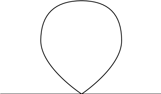
FIG. 2.: ‘Tadpole’ graph containing the only ultraviolet singularity of ${\cal Z}$

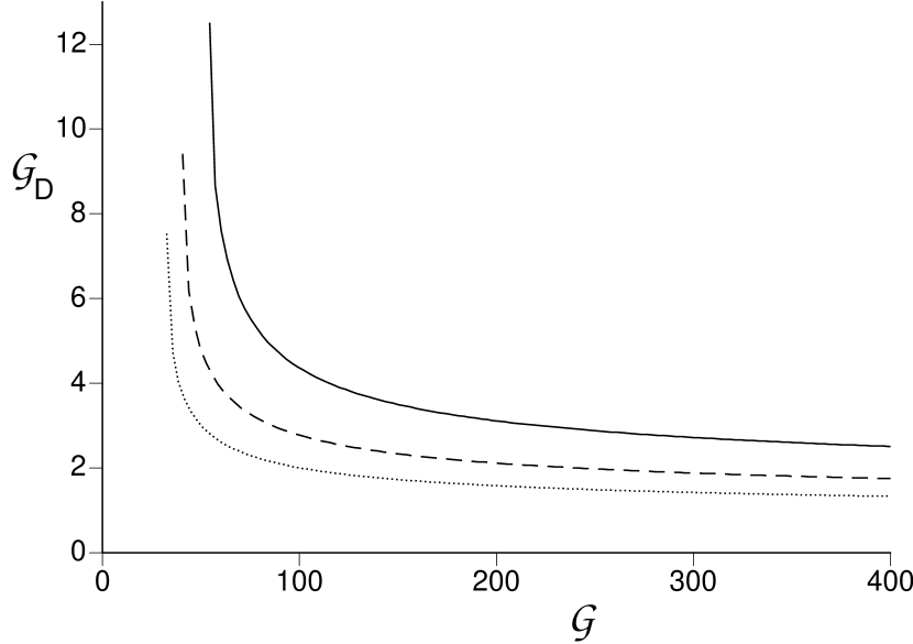
FIG. 3.: The ‘dual’ dimensionless coupling ${\cal G}_{D}$ as a function of ${\cal G}$ for $n=1$ (full line), $n=2$ (dashed line), and $n=3$ (dotted line).

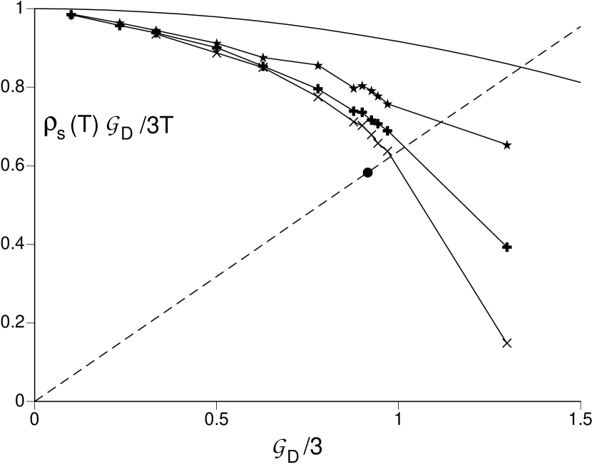
FIG. 4.: Numerical results for $(\rho_{s}(T)/T)/({\cal G}_{D}/3)$ as a function of ${\cal G}_{D}/3$. We used a square lattice of $L\times L$ sites with periodic boundary conditions and lattice spacing $a$. The lattice sizes used were $L=64$ (stars), $L=128$ (pluses) and $L=256$ (X’s). The dashed line is the locus of points where the Nelson-Kosterlitz jump (57) is obeyed. The full line is the result of the small ${\cal G}_{D}$ expansion in (50). The filled circle indicates the position of the Kosterlitz-Thouless transition determined by the extrapolation to $L=\infty$ limit using the method described in the text and in Fig 5. In the approximation in which we assume that the $T$ dependence of ${\cal G}_{D}$ is given by its leading value as $T\rightarrow 0$, ${\cal G}_{D}\approx 3T/\rho_{s}(0)$, the scale on the horizontal axis becomes $T/\rho_{s}(0)$, while that on the vertical axis becomes $\rho_{s}(T)/\rho_{s}(0)$.

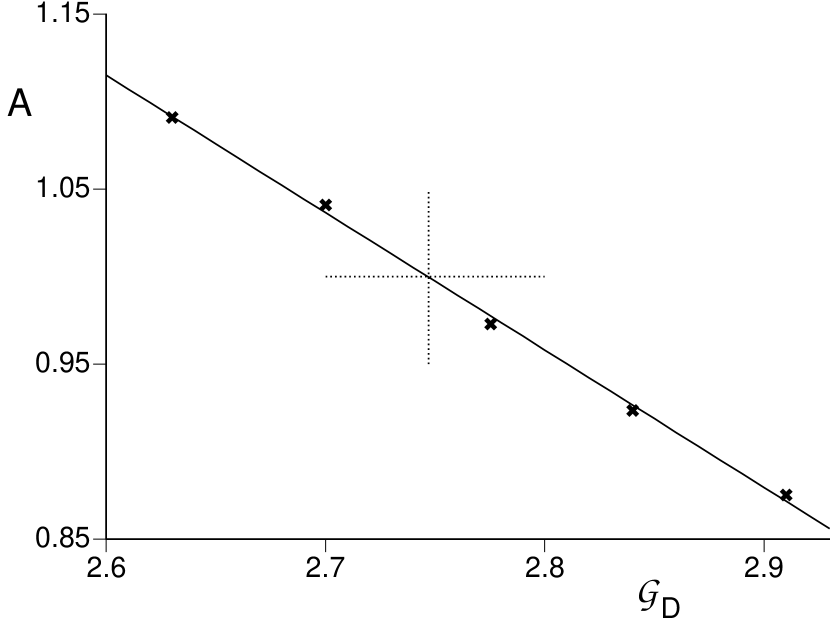
FIG. 5.: Values of the coefficient $A$ in (59) determined by fitting the $L$ dependence of the measured $\rho_{s}(T)/T$ to (59). We fit the value of $A$ to a linear function of ${\cal G}_{D}$, and point where the line has the value $A=1$ (indicated by the dotted lines), determines the position of the Kosterlitz Thouless transition.

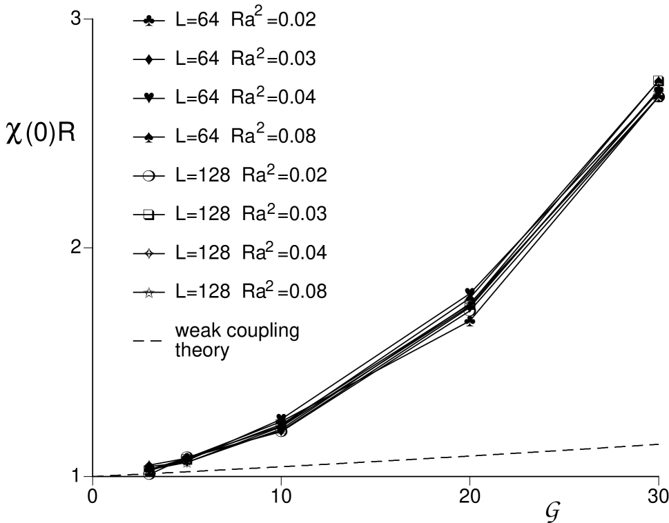
FIG. 6.: Scaling plot of the static susceptibility $\chi(0)$ for $n=3$ as function of ${\cal G}$. The dashed line indicates the prediction of weak-coupling expansion in (34).

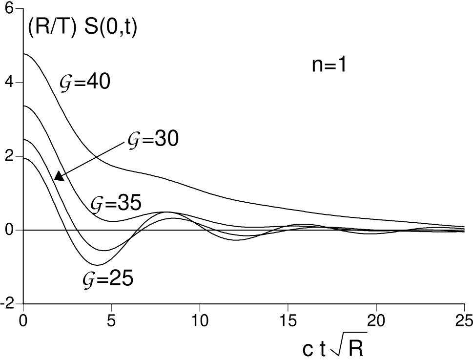
FIG. 7.: The dynamic structure factor in the time domain, $S(k,t)=\int d\omega/(2\pi)S(k,\omega)e^{-i\omega t}$, for $n=1$ and with ${\cal G}=25,30,35,40$.

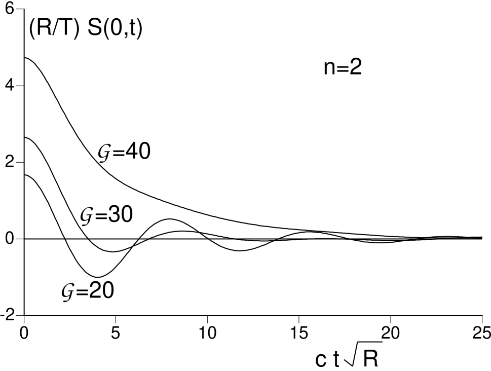
FIG. 8.: As in Fig 7, but for $n=2$ and with ${\cal G}=20,30,40$.

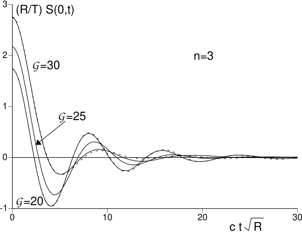
FIG. 9.: As in Fig 7 but for $n=3$ and ${\cal G}=20,25,30$. For ${\cal G}=20,30$ we used two different values of $Ra^{2}$ ($Ra^{2}=0.03,0.04$ for ${\cal G}=20$, and $Ra^{2}=0.04,0.08$ for ${\cal G}=30$) and these are indicated by the presence of both dashed and full lines for these cases. The good agreement between the dashed and full lines is evidence that we are measuring the universal values in the continuum limit.

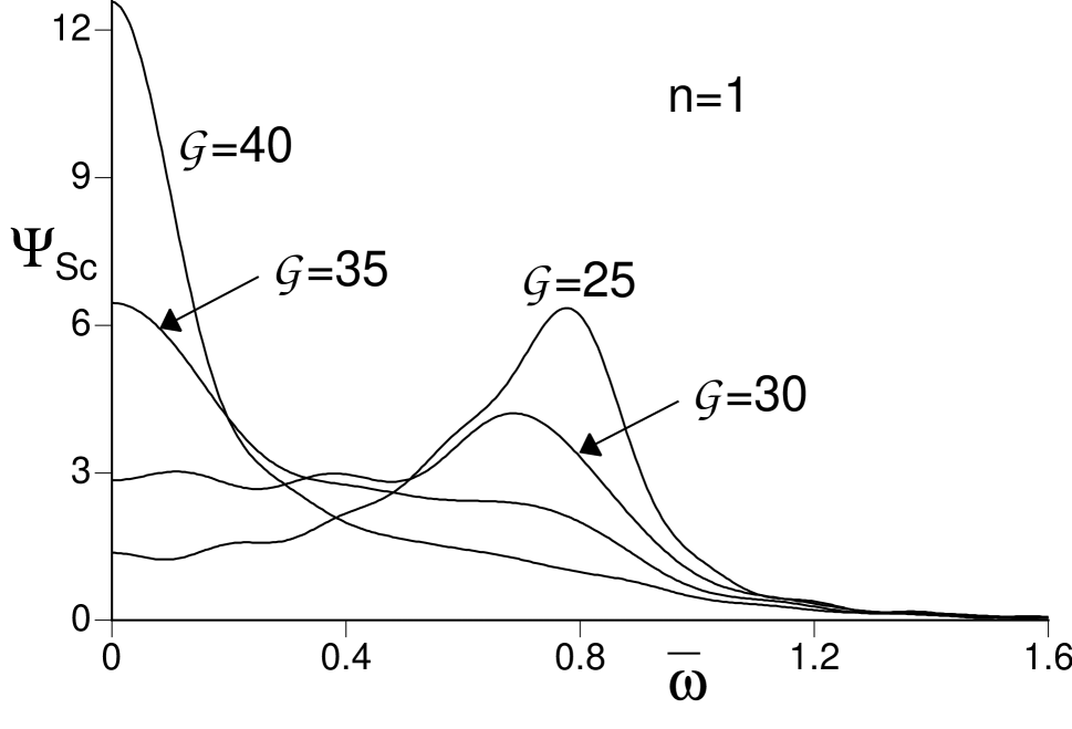
FIG. 10.: The Fourier transform of Fig 7 to frequencies, which yields the scaling function $\Psi_{Sc}(0,\overline{\omega},{\cal G})$ in (32), where $\overline{\omega}=\omega/c\sqrt{R}$. Results are for $n=1$ and ${\cal G}=25,30,35,40$.

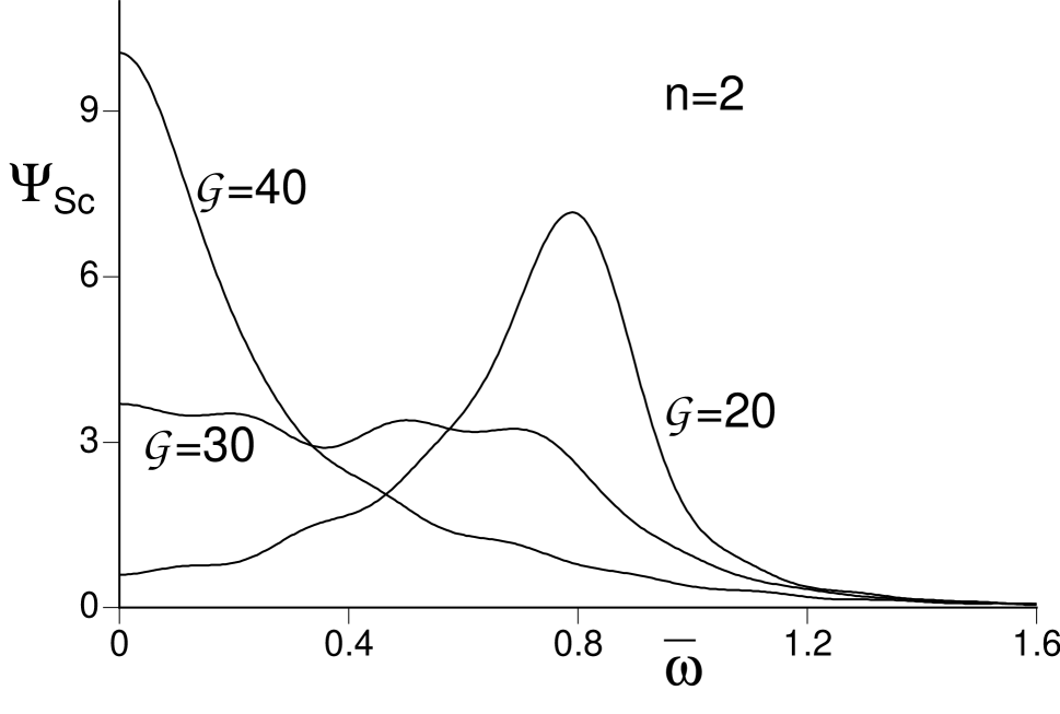
FIG. 11.: As in Fig 10 but for $n=2$ and ${\cal G}=20,30,40$.

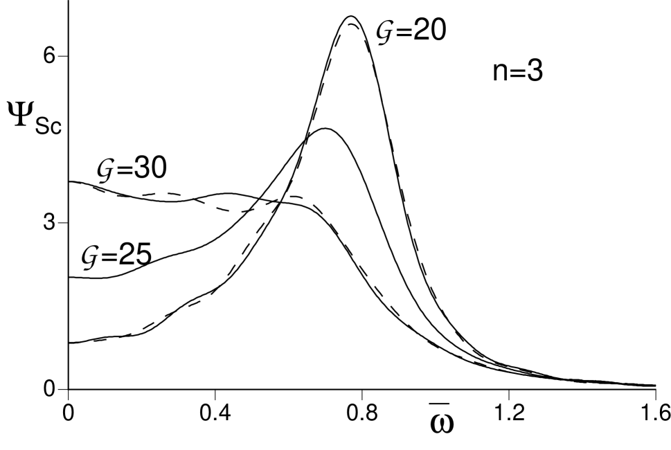
FIG. 12.: As in Fig 10 but for $n=3$ and ${\cal G}=20,25,30$. As in Fig 9, there are two data sets for ${\cal G}=20,30$ (indicated by the dashed and full lines), corresponding to two different values of $Ra^{2}$.

REFERENCES

- [1] G. Aeppli, T. E. Mason, S. M. Hayden, H. A. Mook, and J. Kulda, Science 278, 1432 (1998).
- [2] J. M. Tranquada, J. D. Axe, N. Ichikawa, A. R. Moodenbaugh, Y. Nakamura and S. Uchida, Phys. Rev. Lett. 78, 338 (1997).
- [3] S. Das Sarma, S. Sachdev, and L. Zheng, Phys. Rev. B 58, 4672 (1998).
- [4] V. Pellegrini, A. Pinczuk, B. S. Dennis, A. S. Plaut, L. N. Pfeiffer, and K. W. West, Science 281, 799 (1998).
- [5] W. N. Hardy, S. Kamal, R. Liang, D. A. Bonn, C. C. Homes, D. N. Basov, and T. Timusk in Proceedings of the 10th Anniversary HTS Workshop on Physics, Materials and Applications edited by B. Batlogg et al. (World Scientific, Singapore), p. 223 (1996).
- [6] S. Sachdev, Phys. Rev. B 55, 142 (1997).
- [7] N. Trivedi and M. Randeria, Phys. Rev. Lett. 75, 312 (1995).
- [8] V. J. Emery and S. A. Kivelson, Nature 374, 434 (1995); V. J. Emery and S. A. Kivelson, J. Phys. Chem Solids 59, 1705 (1998).
- [9] M. Franz and A. J. Millis, Phys. Rev. B 58, 14572 (1998).
- [10] H.-J. Kwon and A. T. Dorsey, cond-mat/9809225.
- [11] K. Damle and S. Sachdev, Phys. Rev. B 56, 8714 (1997).
- [12] S. Sachdev, and J. Ye Phys. Rev. Lett. 69, 2411 (1992).
- [13] A. V. Chubukov, S. Sachdev, and J. Ye Phys. Rev. B 49, 11919 (1994).
- [14] P. Ramond, Field Theory, A Modern Primer (Benjamin-Cummings, Reading, 1981).
- [15] W. Loinaz and R. S. Willey, Phys. Rev. D 58, 076003 (1998).
- [16] B. I. Halperin, P. C. Hohenberg, and S. k. Ma, Phys. Rev. Lett. 29, 1548 (1972); Phys. Rev. B 10, 139 (1974).
- [17] P. C. Hohenberg and B. I. Halperin, Rev. Mod. Phys. 49, 435 (1977).
- [18] S.-J. Chang, Phys. Rev. D 13, 2778 (1976).
- [19] S. Chakravarty, B. I. Halperin, and D. R. Nelson, Phys. Rev. B 39, 2344 (1989).
- [20] S. Tyc, B.I. Halperin and S. Chakravarty, Phys. Rev. Lett 62, 835 (1989).
- [21] R. Toral and A. Chakrabarti, Phys. Rev. B 42, 2445 (1990).
- [22] U. Wolff, Phys. Rev. Lett. 62, 361 (1989).
- [23] K. Harada and N. Kawashima, Phys. Rev. B 55, R11949 (1997); J. Phys. Soc. Jpn. 67, 2768 (1998).
- [24] H. Weber and P. Minnhagen, Phys. Rev. B 37, 5986 (1987).
- [25] A. J. Leggett, S. Chakravarty, A. T. Dorsey, M. P. A. Fisher, A. Garg, and W. Zwerger, Rev. Mod. Phys. 59, 1 (1987).
- [26] U. Weiss, Quantum Dissipative Systems (World Scientific, Singapore, 1993).
- [27] F. Lesage and H. Saleur, Nucl. Phys. B 493, 613 (1997).
- [28] S. Sachdev in Highlights in Condensed Matter Physics, Y. M. Cho and M. Virasoro eds. (World Scientific, Singapore); cond-mat/9811110.
- [29] N. Read and S. Sachdev, Phys. Rev. Lett. 62, 1694 (1989).
- [30] B. Keimer, H. F. Fong, S. H. Lee, D. L. Milius and I. A. Aksay, cond-mat/9705103.
- [31] S. Zhang, Science 275, 1089 (1997).
- [32] B. Normand and T. M. Rice, Phys. Rev. B 54, 7180 (1996); ibid 56, 8760 (1997).
- [33] P. Hasenfratz, M. Maggiore, and F. Niedermayer, Phys. Lett. B 245, 522 (1990); P. Hasenfratz and F. Niedermayer, Phys. Lett. B 245, 529 (1990); P. Hasenfratz and F. Niedermayer, Phys. Lett. B 268, 231 (1991).