Disorder, Order, and Domain Wall Roughening in the 2d Random Field Ising Model

Abstract

Ground states and domain walls are investigated with exact combinatorial optimization in two-dimensional random field Ising magnets. The ground states break into domains above a length scale that depends exponentially on the random field strength squared. For weak disorder, this paramagnetic structure has remnant long-range order of the percolation type. The domain walls are super-rough in ordered systems with a roughness exponent $\zeta$ close to 6/5. The interfaces exhibit rare fluctuations and multiscaling reminiscent of some models of kinetic roughening and hydrodynamic turbulence.

PACS #   64.60.Cn, 05.50.+q, 64.60.-i

The random field Ising model attracts interest since it presents an example of competing mechanisms for order and disorder. The local spin couplings favor ferromagnetic ordering whereas variations in the random fields favor disorder. This competition affects thermodynamic properties. Disordered systems are very often governed by the zero-temperature behavior, or the structure and energy of the ground state (GS). In the random field Ising model (RFIM) statistical mechanics of interfaces or domain walls becomes the key question. This is important for finite-temperature dynamics, for coarsening, aging, and fluctuations. The interest is in the scaling and universality in a problem dominated by a complicated, multivalley energy landscape [1, 2].

The effect of dimensionality on order or disorder was solved by Aizenman and Wehr. They proved rigorously that the two-dimensional (2D) RFIM has in the thermodynamic limit no long-range ferromagnetic character [3]. In 3D order was shown to exist at finite temperatures and weak fields [4], and therefore the lower critical dimension of the RFIM is 2. Here we study the transition from order to disorder in the 2D RFIM: ground states and scaling properties of single domain walls with varying system size. The expectation is that the ground state becomes unstable to domain formation at a breakup length scale [5] because of domain wall entropy even at zero temperature. In contrast, a simple energy or Imry-Ma domain argument indicates for weak fields in two dimensions long-range order (if $hL^{d/2}<JL^{d-1}$, where $h$ is the RF strength, $J$ the strength of ferromagnetic couplings, $L$ length scale, and $d$ the dimension) [6, 2]. This fails so that domains, albeit large ones, do exist for arbitrarily weak fields. Existing finite temperature Monte Carlo [7] and exact ground state results [8] do not extend into this regime.

The scaling properties of domain walls is studied here with the domain wall renormalization group (DWRG). One considers DW’s imposed with boundary conditions, and compares to systems without forced DW’s and with the same disorder to find the DW energy. The domain walls are predicted to be self-affine by functional renormalization group calculations and an Imry-Ma argument, with the roughness exponent $\zeta_{d}^{RF}=(5-d)/3$ [9, 10]. $\zeta_{d}^{RF}$ shows, e.g., how the interface width scales, $w\sim L^{\zeta}$ ($w^{2}=\langle z^{2}-{\bar{z}}^{2}\rangle$, where $z$ is the local interface height). In this picture $\zeta$ vanishes at the upper critical dimension and at $d=2$ $\zeta_{2}=1$ [5, 10]. The domain wall energy would concurrently be expected to be linear, $E(L)=E_{0}L+E_{1}L^{\theta}$. The energy fluctuation exponent $\theta$ should obey the exponent relation $\theta=2\zeta+d-3$, similar to the random bond Ising model and directed polymers [11, 1]. The 1+1 -dimensional RF domain wall problem maps in the continuum limit directly to the Kardar-Parisi-Zhang or Burger’s equation, the paradigm of interface models in disordered media [12], so that again $\zeta_{2}=1$ and $\theta_{2}=1$ [13].

The picture of self-affine DW’s has been claimed to be confirmed by both early transfer-matrix calculations [14] and studies using combinatorial optimization [10, 15]. In this Rapid Communication this is shown to be false. The domain walls exhibit rich scaling reminiscent of turbulent behavior as in certain kinetic growth models [16, 17] and in ordinary hydrodynamics [18, 19]. Also, the concept of self-affinity is not valid because of the length scale induced by ground state breakup.

Finding the ground state of the RFIM maps exactly into the minimum cut – maximum flow problem of network or combinatorial optimization [20]. The use of such algorithms, pioneered by Ogielski [21], has recently started become common as one can do exact disorder averages for systems governed by zero-temperature and energy landscape effects [22]. A related problem solvable with the method is the DAFF (diluted antiferromagnet in a field) providing an experimental realization.

The application of combinatorial optimization starts by augmenting the RFIM with two extra sites. The network optimization problem is defined on a graph, in which each edge corresponds to a site in the augmented RFIM. Each of the original sites is connected with one of the two extras, depending on the sign of the local field $h_{i}$. The capacities of the vertices in the graph are equal to either $2J$ or $2|h_{i}|$ for couplings to the extra sites. This is a network flow problem, since the connections equal local flow constraints or capacities. The maximum flow between the extra sites gives the ground state energy, and the division to two spin states among the Ising spins is the minimum cut that results in the maximum flow. This method is exact and does not suffer from metastability like normal Monte Carlo or optimization with simulated annealing. We use an efficient push-relabel preflow-type [23] code. The CPU-time scales as $t_{CPU}\sim N^{1.2}$, with $N\sim L^{2}$ increasing thus almost linearly in $N$. Systems can be studied up to $L=1000$ ($N=10^{6}$).

Figure 1 and the inset show examples of ground states with weak and strong disorder and with domain wall-enforcing or periodic boundary conditions, respectively [24]. The random fields $h_{i}$ obey either a bimodal distribution ($P(h_{i})=\frac{1}{2}[\delta(h_{i}-\Delta)+\delta(h_{i}+\Delta)]$) or a Gaussian one, ($P(h_{i})=1/(\sqrt{2\pi}\Delta)\exp[\frac{1}{2}(h_{i}/\Delta)^{2}]$, $\Delta$ measures the standard deviation, $J=1$). First we characterize the transition from the case of Fig. 1, a ferromagnetic ground state here with an imposed domain wall, to that shown in the inset, with a negligible magnetization. Then the properties of single domain walls are studied.

We make the assumption of one single length scale, proportional to that at which the order vanishes (e.g., the magnetization becomes zero). We measure the probability of a purely ferromagnetic GS, $P_{FM}(L)=P(L,|m|=1)$, as a function of $L$ with fixed $\Delta$. This probability maps for both types of disorder to the magnetization [$m=m(P_{FM})$]. The break-up length scale is defined with $P_{FM}(L)=0.5$. The advantage is that the breakup of the ground state is visible at much smaller $L$ than with other order parameters, making it possible to study breakup to a domain structure with $L\rightarrow\infty$. Other choices could be the cluster size distribution, the spin-spin correlation length, magnetization, and so on. For example, the correlation length shows finite size effects, which might be partly explained below.

$L_{b}$ for this definition is depicted for varying $\Delta$ in Fig. 2. The prediction that the 2D RFIM ground state should have no long-range order is based on the fact that at large enough scales entropy, the many possible configurations available should make the domain wall energy vanish [5]. Our results yield, in agreement, an exponential length scale

$\displaystyle L_{b}\sim\exp{(A[1/\Delta]^{2})},$

where the disorder-dependent constant $A=1.9\pm 0.2$ and $2.1\pm 0.2$ for bimodal and Gaussian disorder, respectively. The definition of $L_{b}$ implies that the magnetization vanishes at a larger $L>L_{b}$. The values of $A$ are different from the ones obtained by finite-temperature Monte Carlo simulations for small $L$ [7]. These results prove that the mechanism for the breakup of the GS is due to entropic effects.

No ferromagnetic order exists in the ensuing domain structure with zero magnetization. For strong disorder one can show that the spin-spin correlation length is proportional to the average cluster size for both $L<L_{b}$ and $L\geq L_{b}$. Here we study the disorder averaged properties of the largest clusters. These are found to percolate and thus give rise to sub-dominant (the weight of the spanning cluster vanishes in the thermodynamic limit) long-range order. For bimodal disorder the fractal dimension is $d_{f}=1.90\pm 0.02$ (Fig. 2 inset), very close to the exact value of standard 2D percolation 91/48. The inset of Fig. 2 also shows the sum over the random fields of the percolation clusters. This sum scales with the same fractal dimension 1.90. Thus the Imry-Ma argument is not true for the largest clusters as the global optimization produces domains whose magnetization is extensive. To summarize for weak disorder there is hidden order in the ground state of the RFIM structure in two dimensions. This is not in contradiction to the exact Aizenman-Wehr-theorem since $m\rightarrow 0$. However, it gives rise to nontrivial correlations in the structure, thus order. For stronger fields there is a crossover to site percolation and a nonpercolating structure (as $p_{c}\sim 0.593$ on a square lattice and now $p=0.5$). The critical $\Delta_{c}$, below which lattice effects are smeared out, is $(h/J)_{c}=2$ for bimodal disorder and $\Delta_{c}=2.1\pm 0.2$ for Gaussian, respectively. The threshold for the Gaussian case is a rough estimate. It would interesting but hard to analyze this percolation transition in detail, since one needs $L>L_{b}$.

Next we turn to interface scaling. Fig. 3 shows the interface width, the interface energy $E$, and the energy fluctuations $\Delta E^{2}=\langle E^{2}-\bar{E}^{2}\rangle$ up to $L=500-1000$. $E$ is obtained in the DWRG sense by subtracting the energy of a ground state from one with an imposed domain wall and identical disorder. $\langle\dots\rangle$ is the average over disorder. We take the Solid-On-Solid (SOS) -limit: in the case of a multiply valued interface the highest location is chosen from the exact interface configurations. The weight of overhangs is negligible for weak disorder and small systems. In the weak-disorder regime the global roughness exponent is found as $\zeta\simeq 1.2\pm 0.05$. As $\zeta>1$ the RF interfaces are super-rough. This is, however, true only up to a length scale, below which the GS has already broken down (see inset, Fig. 1). Above that scale a domain wall becomes fractal, and $\zeta=1$. There is a sharp transition between these two regimes, and the data for $\Delta=10/9$ in the inset of Fig. 3(a) has two regimes corresponding to “ferromagnetic” and “disordered” ground states. Figure 3(b) shows the DWRG result for the DW energy: there is a logarithmic correction to the DW energy in the FM phase. In the paramagnetic phase the energy has only a remnant contribution from the boundary conditions. For the FM phase the energy fluctuation exponent is $\theta\simeq 1$. The values for the exponents $\zeta$ and $\theta$ disagree with the exponent relation $\theta_{2d}=2\zeta_{2d}-1$ [11].

If one studies interfaces based either on a mapping to the Burgers’-KPZ equation or functional RG calculations these depend on the small slope approximation, which is a problem if $\zeta\simeq 1$. Fig. 4 shows the statistics of interface fluctuations in the form of the interface step height probability density function (PDF) $f(\Delta z_{i,i+1},L)$. $\Delta z_{i,i+1}$ is the height difference between two neighboring sites ($z_{i}$) along the SOS interface ($i=1,\dots,L$). The $f(\Delta z,L)$ show stretched exponential behavior. The PDF’s are clearly $L$ dependent, but only up to the breakup length scale for interfaces. The height differences resemble velocity gradients or energy dissipation in fluid turbulence and behavior in interface growth problems [16, 17, 25, 18] that are governed by intermittent, rare events. The step height fluctuations are not restricted to the exact interfaces. A SOS transfer matrix calculation (allowing for $\Delta z>1$) reproduces these features, and demonstrates that the interpretation of Ref. [14] is wrong since the true scaling behavior is super-rough at, also, low temperatures. A multifractal study of the average step height $|\Delta z|$ and the interface height-height correlation functions $G_{k}(r)=\langle|h(l)h(l+r)|^{k}\rangle$ indicates that the local interface scaling is multiaffine, e.g., $G_{k}(r)\sim A_{k}r^{\alpha_{k}k}$. For instance, $\alpha_{k}\simeq 0.88,\dots,0.9$ for $k=1$, but for already $k=2$ $\alpha_{k}\simeq 0.66$ with the exponent being a weak function of $L$ at fixed $\Delta$. The higher exponents $\alpha_{k}$ decrease with $k$ and increase with $L$ for moderate $L$. Thus, there is another analogy between height-height correlations of the RFIM and velocity-velocity correlations in turbulence. Both the amplitude of $G$ ($A_{k}$) and $|\Delta z|$ do not self-average but scale with $L$ and $\Delta$. It is tempting to draw a parallel with $L_{b}$ in here and the outer length scale of turbulence. In both cases the largest length scale is fixed by external conditions: the strength of randomness or the Reynolds number [26]. The correspondence is not one-to-one, however, since the scaling properties depend on both $L_{b}$ and $L$ (Fig. 4).

In conclusion, we demonstrate the breakdown of the ground state, at zero temperature, in the 2D random field Ising model. There is however hidden, long-range order in the form of the spanning cluster that seems first contradictory to destroyed ferromagnetic order. This arises by “entropic optimization” so that the cluster magnetization becomes extensive. The annihilation of order with increasing sample size is reflected in the properties of domain walls. For small systems and weak fields the domain walls are super-rough, with a roughness exponent that is well in excess of analytic estimates. This can be traced to “turbulent” rare interface fluctuations, but in an equilibrium system in contrast to models of kinetic surface roughening or Navier-Stokes turbulence. In large systems the concept of an individual domain wall becomes ill-defined. The domain wall energy has a logarithmic correction: one should study how far this lack of self-affinity penetrates the GS energy landscape properties and, perhaps, dynamical behavior. It will be interesting to see if the nonstandard interface scaling properties persist in higher dimensions or in the presence of an applied field. We believe that this is so in the latter case, though the ground states are naturally ferromagnetic. This would have consequences for driven interfaces below the crossover to annealed disorder for a strong enough driving force [25, 27].

This work has been supported by the Academy of Finland (MATRA and M. J. A.).

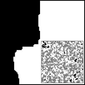
FIG. 1.: Two typical examples of RFIM ground states with periodic and forced boundary conditions. Weak bimodal disorder, $\Delta=10/17,L=100$. Note the large jumps on the interface and the lack of overhangs. The interface is the boundary between the black/white domains (different spin states). Inset shows a strong Gaussian disorder case, $\Delta=2$. Spins that point “down” in the ground state are drawn white. The “up” spins are black or grey if in the largest (percolation) cluster.

FIG. 2.: $L_{b}$ vs. $(1/\Delta)^{2}$ for bimodal and Gaussian disorder (closed circles and open squares, respectively), calculated from $P_{FM}(L_{b})=0.5$. $\Delta=h/J$ for binomial and $\Delta=\delta h$ for Gaussian disorder. The inset shows the average mass of spanning clusters for bimodal $\Delta=25/13$ up to $L=470$ (open diamonds). The plot shows also the sum of the random fields of the sites belonging to the same clusters (closed triangles). The 2D percolation fractal dimension $d_{f}=$ 91/48 is indicated with a line.

FIG. 3.: (a) Scaling of the global interface width for bimodal disorder. $\Delta=$ 2/3 (open triangles) and 3/2 (closed squares). The line indicates a least-squares fit with a roughness exponent $\zeta=$ 1.20 $\pm$ 0.05. The inset shows the crossover in interface properties with increasing system size ($\Delta=$ 10/9). (b) Scaling of the energy (per length) for bimodal $\Delta=$ 1/3 (open circles) and 5/12 (closed squares). The inset shows the scaling of energy fluctuations for $\Delta=$ 1/3.

FIG. 4.: Interface step probability density function for $h/J=1/2$, $L=20,40,100,200,480$. For simplicity the data includes only those steps that do not involve local overhangs.

REFERENCES

- [1] T. Halpin-Healy and Y.-C. Zhang, Phys. Rep. 254, 215 (1995).
- [2] Spin Glasses and Random Fields, edited A. P. Young (World Scientific, Singapore, 1998).
- [3] M. Aizenman and J. Wehr, Phys. Rev. Lett. 62, 2503 (1989).
- [4] J. Bricmont and A. Kupiainen, Phys. Rev. Lett. 59, 1829 (1987).
- [5] K. Binder, Z. Phys. B 50, 343 (1983); G. Grinstein and S.K. Ma, Phys. Rev. B 28, 2588 (1983).
- [6] Y. Imry and S.-K. Ma, Phys. Rev. Lett. 35, 1399 (1975).
- [7] J.F. Fernandez and E. Pytte, J. Appl. Phys. 57, 3274 (1985).
- [8] J. Esser, U. Novak, and K.D. Usadel, Phys. Rev. B 55, 5866 (1997).
- [9] D. Fisher, Phys. Rev. Lett. 56, 1964 (1986).
- [10] E.D. Moore, R.B. Stinchcombe, and S.L.A. de Queiroz, J. Phys. A 29, 7409 (1996).
- [11] D.A. Huse and C.L. Henley, Phys. Rev. Lett. 54, 2708 (1985).
- [12] M. Kardar, G. Parisi, and Y.-C. Zhang, Phys. Rev. Lett. 56, 889 (1986).
- [13] Y.-C. Zhang, J. Phys. A19, L941 (1986).
- [14] J.F. Fernandez et al., Phys. Rev. Lett. 51, 203 (1983).
- [15] M. Jost, U. Nowak, and K. Usadel, Phys. Status Solidi B202, R11 (1997).
- [16] J. Krug, Phys. Rev. Lett. 72, 2907 (1994).
- [17] S. Das Sarma et al., Phys. Rev. E53, 359 (1996).
- [18] P. Kailasnath, K. R. Sreenivasan, and G. Stolovitzky, Phys. Rev. Lett. 68, 2766 (1993); S. Grossmann and D. Lohse, Europhys. Lett. 21, 201 (1993). D. Lohse and S. Grossmann, Physica A 194, 519 (1993).
- [19] U. Frisch, Turbulence (Cambridge University Press, Cambridge, England, 1995).
- [20] F. Barahona, J. Phys. A18, L673 (1985); J.C. Angles d’Auriac, M. Preissmann, and R. Rammal, J. Phys. (France) Lett. 46, L173 (1985).
- [21] A. T. Ogielski, Phys. Rev. Lett. 57, 1251 (1986).
- [22] M. Alava, P. Duxbury, C. Moukarzel, and H. Rieger, to appear in Phase Transitions and Critical Phenomena, edited C. Domb and J. Lebowitz.
- [23] A.V. Goldberg and R.E. Tarjan, J. Assoc. Comput. Mach. 35, 921 (1988).
- [24] Spins are set up or down at opposing boundaries to enforce the domain wall, with no regard of the local fields.
- [25] S. Galluccio and Y.-C. Zhang, Phys. Rev. E 51, 1686 (1995).
- [26] See also J.P. Bouchaud, M. Mézard, and G. Parisi, Phys. Rev. E 52, 3656 (1995).
- [27] H. Ji and M. Robbins, Phys. Rev. A 44, 2538 (1991); T. Nattermann et al., J. Phys. (France) II 2, 1483 (1992); H. Leschhorn, Physica A195, 324 (1993); O. Narayan and D.S. Fisher, Phys. Rev. B48, 7030 (1993); D. Ertaş and M. Kardar, Phys. Rev. E 49, R2535 (1994).