Long-range coherence and mesoscopic transport in N-S metallic structures

Abstract

We review the mesoscopic transport in a diffusive proximity superconductor made of a normal metal (N) in metallic contact with a superconductor (S). The Andreev reflection of electrons on the N-S interface is responsible for the diffusion of electron pairs in N. Superconducting-like properties are induced in the normal metal. In particular, the conductivity of the N metal is locally enhanced by the proximity effect. A re-entrance of the metallic conductance occurs when all the energies involved (e.g. temperature and voltage) are small. The relevant characteristic energy is the Thouless energy which is $\hbar$ divided by the diffusion time for an electron travelling throughout the sample. In loop-shaped devices, a $1/T$ temperature-dependent oscillation of the magnetoresistance arises with a large amplitude from the long-range coherence of low-energy pairs.

1 Introduction

The ability to fabricate small samples, thanks to the progress of the technology developped for the microelectronic industry, has opened a new field of research for the physics community. This field of research has been called mesoscopic physics since although the size of these systems is far bigger than the atomic scale, quantum mechanics is needed in order to understand their behavior. A new length scale has then been introduced, intermediate between the atomic scale and the macroscopic scale, namely the phase-breaking length $L_{\varphi}$ [1, 2]. In pure metals at low temperature, $L_{\varphi}$ can reach several micrometers [3, 4].

The best known examples of mesoscopic physics are the universal conductance fluctuations and the weak localization. The first effect arises from the interference of the one-electron wave-function using all the possible paths to travel through the sample. This interference gives rise to magnetoconductance fluctuations, whose amplitude $\Delta G=e^{2}/h$ has the remarkable property to be universal, i.e. independent of the sample conductance. In a loop geometry, this interference gives rise to the well known Aharonov-Bohm oscillations with a flux-periodicity $2\phi_{0}=h/e$ [5].

In cylinder or arrays geometries with a total length exceeding $L_{\varphi}$, Aharonov-Bohm oscillations and universal conductance fluctuations average to zero. But at low magnetic field, a special class of event survives to ensemble averaging. When one considers a given path and its time reversed dual, the wave-functions along the two paths interfer constructively if time reversal symmetry is conserved [6]. In that special case, interferences increase the probability to return to the origin of a loop, and one observes a decrease of the conductance. For the loop geometry, the flux periodicity is $\phi_{0}=h/2e$ since the loop is travelled twice by the electron [7].

Both conductance fluctuations and weak localization are mesoscopic effects in the sense that they appear on the length scale of the phase-breaking length $L_{\varphi}$. Their amplitude corresponds to the conductance ($e^{2}/h$) of one transport channel, even if many channels are involved. This comes from the fact that the different channels do not have a common phase reference. In the usual case of a sample made of an evaporated thin metallic film, the amplitudes of conductance fluctuations and weak localization are small compared to the total conductance.

The mesoscopic effects are not intrinsically limited to a small amplitude. The most beautiful example is the ”mesoscopic superconductivity” arising in a normal metal N from the Andreev reflection of electrons at a superconductor S. The superconductivity in S results in a macroscopic phase-coherent pair condensate. In these N-S systems, the coupling of normal electrons to the pair condensate induces coherence effects which add constructively and reach a total large amplitude.

In this review paper, we will discuss the transport properties of devices made of a normal metal in metallic contact with a superconductor. This scientific area has met a remarkable new interest in the recent years, due to novel experiments on samples with new mesoscopic designs [8, 9, 10]. Here, we will restrict to the case of transport in diffusive metals in the presence of Andreev reflection. The Josephson effect [11, 12] will not be discussed as we will concentrate on non-equilibrium properties. We will focus on the regime where the resistance of the N-S interface is negligeable compared to the metallic resistance of the wire.

2 An introduction to the quasiclassical theory of the proximity effect

2.1 The Andreev reflection

Let us consider a sample made of a normal metal in contact with a superconductor. At a temperature well below the superconducting transition of S and at low bias voltage, the thermal energy $k_{B}T$ and the electrostatic energy $eV$ are much smaller than the gap of S. As a consequence, normal electrons arriving on the N-S interface cannot find any available states in S and are Andreev-reflected [13].

In the Andreev reflection, the electron is reflected as a hole, while a Cooper pair is transmitted in the superconductor, see Fig. 1. The spin and every component of the electron momentum are reversed. In this scope, a N-S interface is similar to a phase-conjugating mirror in optics. As it has the opposite momentum, the reflected hole traces back the path of the incident electron. The phase acquired by the electron is ”eaten up” as the hole retraces back the trajectory of the incident electron.

The electron and the hole do not form a pair since they are not present at the same time in the metal, but the Andreev reflection correlates two electron states in N. The reflection of the hole may also be seen as the absorption of an electron by the superconductor. In this scope, two electrons travel on the same path through the N metal and are absorbed as a Cooper pair in S. This effect can be reversed, so that an electron pair from S can diffuse in the N metal. In the following, we will indifferently use both languages : reflection of an electron into a hole (and vive-versa) or diffusion of an electron pair in N.

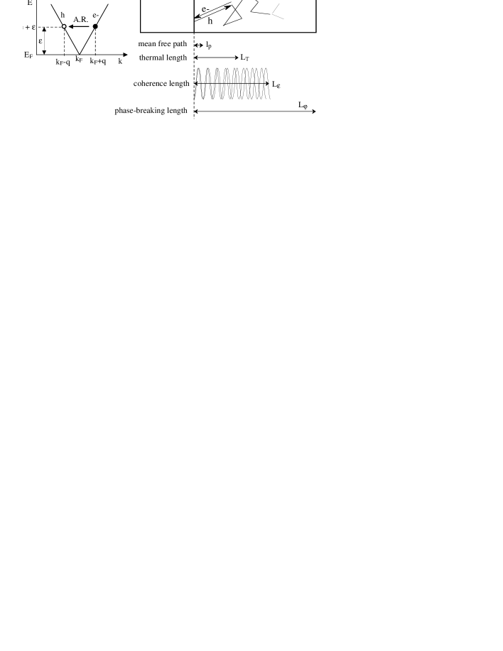
Fig.  1: Left : Schematic of the Andreev reflection process. An electron with a small extra energy $\epsilon$ compared to the Fermi energy $E_{F}$ arrives from the N side on the N-S interface. There is a wave-vector mismatch of $2q$ between the incident electron and the reflected hole. Right : Relevant length scales with their schematic respective amplitude in a metallic thin film. The energy-dependent coherence length $L_{\epsilon}$ is the length over which the two components of the electron pair acquire a phase difference of order $\pi$.

If one looks more precisely, the reversal of the electron momentum is perfect only at the Fermi level. Let us consider an electron with a small extra energy $\epsilon$ with respect to the Fermi level energy $E_{F}$. Its wave-vector $k_{e}=k_{F}+q$ slightly differs from the Fermi wave-vector $k_{F}$. The reflected hole has a slightly different wave-vector $k_{h}=k_{F}-q$, see Fig 1. The incident electron and the reflected hole have a difference $\delta k$ in the perpendicular component of the wave-vector so that :

$$\delta k=2q=k_{F}\frac{\epsilon}{E_{F}}.$$ (1)

Let us now focus on the case where the normal metal is in the dirty limit. This limit is valid when the coherence length of electron pairs (defined below) is much larger than the elastic mean free path. We will also assume that the phase-breaking length $L_{\varphi}$ is much larger than the sample length $L$. By diffusing over a distance $L$ in N, the phase difference between the two electrons of the diffusing pair increases monotonically. After diffusion during a time $t$ over a distance $L\simeq\sqrt{Dt}$ from the interface, the phase shift is :

$$\delta\varphi=\frac{L^{2}}{L_{\epsilon}^{2}},$$ (2)

where we introduce the energy-dependent coherence length :

$$L_{\epsilon}=\sqrt{\frac{\hbar D}{\epsilon}},$$ (3)

$D$ being the diffusion coefficient in N. The Eq. 2 means that the phase drift between the two components of the diffusing pair will be small as long as $L$ is small compared to $L_{\epsilon}$. In this regime, the two electrons are scattered in the same way by impurities and their trajectories are quite the same. As a consequence, the two electrons appear as linked in pair.

At a distance of the order of $L_{\epsilon}$, the phase difference is non-negligeable. At the same time, the trajectories of the electron and the hole are separated by a distance or order of the Fermi wavelength [14]. Further scattering of the two particles will therefore be decorrelated and the pair will break apart. For this reason, we call $L_{\epsilon}$ the coherence length of the electron pair.

It is remarkable that the coherence length $L_{\epsilon}$ coincides with the thermal length $L_{T}$ at the energy $\epsilon=2\pi k_{B}T$. The length $L_{T}$ is usually given in the textbooks [15] as the characteristic decay length for the proximity effect. The thermal length $L_{T}$ is characteristic of a thermal equilibrium electron distribution while the coherence length $L_{\epsilon}$ is characteristic of electrons at a given energy. At the Fermi level, the coherence length $L_{\epsilon}$ is infinite, independently of temperature. The actual coherence length is limited by the phase-breaking length $L_{\varphi}$ of a single electron. In conclusion, the effective coherence length of an electron pair in N varies from about the thermal coherence length $L_{T}$ (at $\epsilon=2\pi k_{B}T$) to the phase-coherence length $L_{\varphi}$ at low energy (at $\epsilon=0$).

The phase drift between the electron and the reflected hole can also be written as :

$$\delta\varphi=\frac{\epsilon}{\epsilon_{c}}$$ (4)

where

$$\epsilon_{c}=\frac{\hbar D}{L^{2}}$$ (5)

is the Thouless energy of a sample of length $L$. The interpretation of Eq. 4 is again very simple. At a given distance $L$, only electrons with an energy below the Thouless energy $\epsilon_{c}$ are still correlated in pairs.

2.2 The Usadel equations

The diffusion of superconductivity in any inhomogenous structure can be described by the Gorkov Green’s functions. In the limit where all the experimentally-relevant length scales are much larger than the Fermi wavelength, the simplification of this fully quantum theory into the quasiclassical theory is valid. In the diffusive regime where the elastic mean free path is small, the Usadel equations [16] are obtained. In this framework, the weak localization effects and the conductance fluctuations are neglected.

The quasiclassical theory has been developped in its full integrity by many groups [17, 18, 19, 20, 21, 22]. A review of the applications of this theory to the field of mesoscopic superconductivity is included in this volume [23]. Here we would like to present a simplified version that keeps the essential physical features of the original theory. For instance, it is very convenient to linearize the Usadel equation. This is acceptable in most of the experimental situations as far as the distance from the interface is not too small compared to the thermal length $L_{T}$ [24]. In this case, the Usadel equations reduce to an equation for the pair amplitude $F$ in the normal metal :

$$\hbar D\,\partial^{2}_{x}F+\{\,2i\epsilon-\frac{\hbar D}{L_{\varphi}^{2}}\,\}F=0$$ (6)

The pair amplitude $F$ is a two-variables function of the position $x$ and the energy $\epsilon$. We neglected here the pairing interaction in N and the inelastic scattering. The Eq. 6 can be intuitively understood as a diffusion equation for the pair amplitude. From the equation, one can derive the following facts : (i) the natural length scale of the pair amplitude diffusion is $L_{\epsilon}$ ; (ii) the diffusion is bound by an exponential cut-off at the distance $L_{\varphi}$. These features confirm our previous qualitative discussion.

Fig.  2: Plot of the imaginary and real part of the pair amplitude wave-function $F(\epsilon,x)$ calculated in the framework of the linearized Usadel equation. The horizontal axis can be read either as the distance $x$ normalized to the energy-dependent coherence length $L_{\epsilon}$ (here the energy $\epsilon$ is fixed) or as the square root of the energy $\epsilon$ in units of the local energy scale $\epsilon_{x}=\hbar D/x^{2}$ related to the distance $x$ (here the distance $x$ is fixed). Inset : the considered sample geometry made of an unfinite N wire in contact with a superconductor S.

As an exemple, let us consider the case of a quasi-1D sample made of a long normal metal wire in perfect contact with a superconducting island, see Fig. 2 inset. The phase-breaking length $L_{\varphi}$ is assumed to be infinite. Solving the Usadel equation, one can obtain the pair amplitude as a complex function $F(\epsilon,x)$ of both the distance x from the S interface and the energy $\epsilon$. Fig. 2 shows the analytically-calculated real and imaginary parts of the pair amplitude. The units of the horizontal axis can be read either as the distance x from the S interface in units of the coherence length $L_{\epsilon}$, or as the square root of the energy $\epsilon$ above the Fermi level in units of the local energy scale $\epsilon_{x}=\hbar D/x^{2}$ related to the distance $x$. This energy scale coincides with the Thouless energy for $x=L$.

As any of the two variables (energy or position) increases, the imaginary part of $F(\epsilon,x)$ decays in an oscillating way, see Fig. 2. This is true when one fixes the energy $\epsilon$ and let the distance $x$ from the S interface grow, or if one fixes the distance $x$ and let the energy $\epsilon$ grow. The energy scale and length scales of decay are respectively $\epsilon_{x}=\hbar D/x^{2}$ and $L_{\epsilon}=\sqrt{\hbar D/\epsilon}$. The measurement of the local density of states [25, 26] or of the magnetic screening [27] gives a direct experimental access to the imaginary part of $F$.

The proximity effect on dissipative transport is connected to the real part of the pair amplitude. From Fig. 2, the real part is zero at the S interface and/or at zero energy. At fixed distance and variable energy, it is maximum at the energy $\hbar D/x^{2}$. At a fixed energy, the real part is maximum at the distance $L_{\epsilon}$ from the interface. At high energy, the real part also decays in an oscillating way. As we will see in the following, the peak at energy $\epsilon\simeq\epsilon_{c}$ in the real part of $F$ is responsible for the re-entrance effect.

2.3 The spectral conductance

In the quasiclassical theory, the coherent transport can be described by a local conductivity. The proximity effect results in a local conductivity enhancement $\delta\sigma$ which is connected to the real part of the pair amplitude $F$ :

$$\delta\sigma(\epsilon,x)=\sigma_{N}(Re[F(\epsilon,x)])^{2}$$ (7)

for small $F$, $\sigma_{N}$ being the normal-state conductivity. Let us note that this excess conductivity is energy-dependent and always positive : the conductance will always increase due to the proximity effect.

Coming back to the sample geometry of Fig. 2, we can draw some conclusions concerning the energy dependence of the sample conductivity. Starting from the zero-energy where the normal-state conductivity is recovered, the conductivity is enhanced by about $25\%$ at the maximum located at $\epsilon\simeq\hbar D/x^{2}$. At higher energy, the excess conductivity decay as $1/\sqrt{\epsilon}$. The most striking prediction is that the normal-state conductivity is recovered at zero energy. It is the origin of the re-entrance effect.

The spectral conductance $g(\epsilon)$ is defined as the conductance for electrons with a given energy $\epsilon$ above the Fermi level flowing through the sample. It can be calculated using the classical circuit theory. In a quasi 1D geometry, it is equal to the wire section S divided by the integral of the local resistivity over the sample length $L$ :

$$g(\epsilon)=S[\int_{0}^{L}{\frac{1}{\sigma_{N}+\delta\sigma(\epsilon,x)}dx}]^{-1}$$ (8)

The spectral conductance is experimentally accessible as it coincides with the zero-temperature limit of the differential conductance at finite bias :

$$G(V=\epsilon/e,T=0)=g(\epsilon)$$ (9)

At finite temperature and zero bias, the measured conductance is essentially an integration over a thermal window of width $k_{B}T$ :

$$G(V=0,T)=\int_{-\infty}^{\infty}g(\epsilon)[4k_{B}T\,{cosh}^{2}(\epsilon/2k_{B}T)]^{-1}d\epsilon$$ (10)

As an example, let us consider the case of a N metalic wire of length $L$ inserted between a N reservoir and S island. The spectral conductance has a maximum of $15\%$ of the normal-state conductance at an energy of about 5 times the Thouless energy $\hbar D/L^{2}$ [21]. At zero energy, the spectral conductance is equal to the normal-state conductance. This effect has been called the re-entrance effect since, coming from the finite energy or temperature regime, there is a re-appearance of the plain metallic conductance at zero energy. This result can be exactly derived from the full Usadel equations [17, 18, 19, 21, 22]. It is also in agreement with the prediction of the random matrix theory [28] and Bogoliubov-de Gennes equations [19].

3 The re-entrance effect

3.1 The experimental observation

In our study, we have focused on the case of noble metals like Cu evaporated in thin films. In these systems, the elastic mean free path $l_{e}\simeq\,10nm$ is quite small. The Thouless energy is about $2\,\mu eV\simeq 20\,mK$ for a sample length of $1\,\mu m$. The thermal length $L_{T}$ is of the order of $100\,nm$ at 1K. The phase-breaking length $L_{\varphi}\simeq 1\mu m$ is approximately constant in our temperature range ($T<1\,K$). Let us note that the elastic mean free path and phase-breaking length scales are quite different in evaporated thin metallic films. This is a major advantage of noble metals compared to doped semiconductors, because one can easily distinguish which length scale is related to a given physical effect.

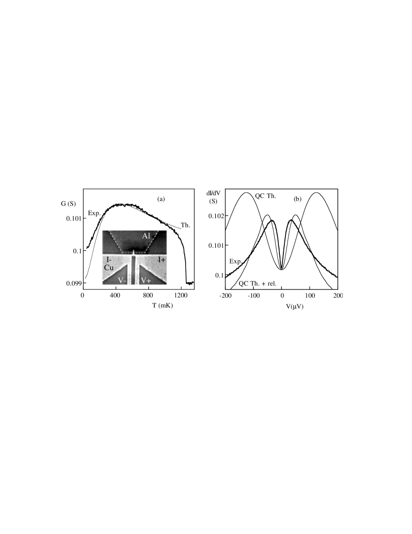
Fig.  3: (a) : Inset shows the micrograph of a typical sample. A dotted white line which follows the edges of the Al island has been drawn for clarity. Main figure : temperature dependence of the conductance measured between the two Cu reservoirs. The experimental curve (Exp.) is shown in parallel with the theoretical curves (Th.). The theoretical curves have been calculated with the non-linear Usadel equation taking into account the finite gap of the superconductor. The phase-breaking length is considered as infinite. (b) Voltage dependence of the differential conductance of the same sample. Compared to the plain theoretical curve (QC Th.), the theoretical curve labeled (QC Th. + rel) includes the additional effect of relaxation in the reservoirs.

Fig. 3a inset shows the micrograph of the sample we will consider [29]. This T-shaped sample is made of three Cu arms joining three wide pads : two are made of Cu, one is of Al. Thin films of Al are superconducting below about 1.3 K. The Cu-Al interface has been carefully prepared in order to obtain a highly transparent interface. Each of the pads is connected to a voltage and a current probe. We will present measurement of the conductance measured between the two Cu reservoirs. With this geometry, we can assert that the current redistribution in the vicinity of the Cu-Al interface due to the superconductivity of Al [30] has a negligeable effect on the measured conductance.

Fig. 3 shows the temperature dependence of the conductance measured with a low bias voltage. As the temperature decreases below the superconducting transition of Al, the conductance first rises. It afterwards reaches a maximum and eventually decreases down to the lowest temperature. The same kind of behaviour can be seen in the voltage dependence of the differential conductance. The differential conductance exhibits a minimum at zero bias, a maximum at a finite bias voltage and then a decrease at large bias.

This experiment provides the proof for the re-entrance of the metallic conductance in a mesoscopic proximity superconductor. A similar effect has been observed in other metallic samples [31] and semiconductor-superconductor structures, the semiconductor being a two-dimensional electron gas [32]. Here, we have been able to track the re-entrance effect as a function of both temperature and voltage and, as discussed in the following, to describe quantitatively our data with the theory.

3.2 Comparison with the theory

We used the quasiclassical theory to quantitatively describe the experimental results. The full non-linear Usadel equations were solved numerically in the precise sample geometry. In both Fig. 3a and b, calculated curves are shown in comparison of the experimental one. The physical parameters used in the calculation match the experimental values and are the same in $G(T)$ and $dI/dV(V)$ data. The Thouless energy used in the calculation is $\epsilon_{c}=15.5\,\mu eV$ and corresponds to a temperature $\epsilon_{c}/k_{B}=180\,mK$. Due to the geometry of the sample, the maximum of the spectral conductance is expected at $3.8\,\epsilon_{c}$. We took into account the finite amplitude of the gap in S, as it is not much larger than the sample Thouless energy.

The temperature dependence data are well fitted by the theoretical calculation. The main difference is at zero energy and zero temperature, where one expects the normal-state value of the conductance. This is not exactly the case in the experiment. This may be an effect of the interactions in the normal metal [18, 24].

In the voltage dependence data, there is a large discrepancy between the experimental and the calculated curves. We found it was necessary to take into account the energy relaxation in the reservoirs [24] : if heating of the reservoirs due to the bias current is included, one recovers a fairly good agreement.

3.3 Discussion

When one integrates the spectral conductance for a thermal distribution of electrons, one finds that the conductance change is analog to the effect of superconductivity over a length $L_{T}$ from the interface [20]. The total conductance change then varies as $1/\sqrt{T}$ with temperature $T$. This does not mean that this region exhibits full superconducting properties. The re-entrance effect brings the counter-proof of it, since at zero temperature and zero bias, the proximity effect on conductance vanishes.

From the theoretical point of view, it is clear that the peak of the real part of $F(\epsilon,x)$ at finite energy (see Fig. 2) describes perfectly the re-entrance effect. A more physical explanation of the re-entrance effect is not an easy task. If one looks at the behaviour of the conductivity at a given energy throughout the sample, the conductivity is the normal-state one both near the interface and far away in the sample. The peak appears in the vicinity of the distance $L_{\epsilon}$ from the S interface. Strikingly, it is the point where the electron pairs break. Everything happens as if it were the breaking of the pairs into two free electrons which is responsible for the conductivity enhancement.

4 Long-range coherence

4.1 An interference experiment

Interference experiments are very useful to distinguish the small coherent contribution from a large background in a complex system. The Aharonov-Bohm geometry allows a direct control of the phase shift by an external magnetic flux. We fabricated a Cu loop-shaped sample which is locally in contact with two Al islands, see Fig. 4b inset. The sample fabrication was such that the interface transparency is very high (see Ref. [33] for details). Let us point out that in all the described measurements, only the conductance of the N metal is measured since the bias current flows through the N wire only. There is no net current through the N-S junctions.

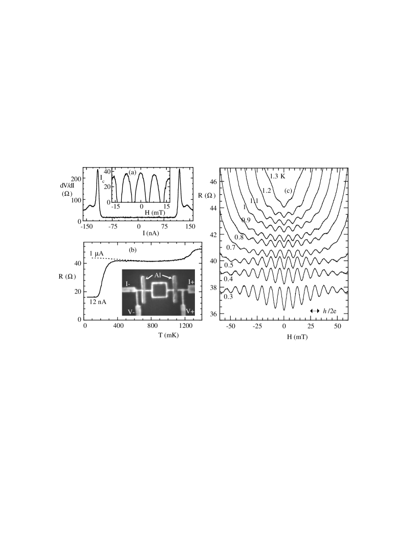
Fig.  4: (a) Sample differential resistance dependence on the bias current at 40 mK. Inset shows the critical current (in nA) measured at 150 mK with a $25\Omega$ differential resistance criteria as a function of the magnetic field. Flux periodicity of the critical current oscillations is $h/2e$. (b) Temperature dependence of the sample resistance with a measurement current 12 nA and 1 $\mu A$. Inset : Micrograph of a typical sample made of a Cu square loop with 4-wire measurement contacts, in contact with two Al islands (vertical). Size of the loop is 500 X 500 $nm^{2}$, width 50 nm, thickness 25 nm. Centre-to-centre distance between the 150 nm wide Al islands is 1 $\mu m$. The length L of the N part of the S-N-S junction is 1.35 $\mu m$. The elastic mean free path is 16 nm, the thermal coherence length is 99 nm at 1 K and the phase-breaking length is about 1.9 $\mu m$. (c) : Low-field magnetoresistance for T = 0.3; 0.4; 0.5; 0.7; 0.8; 0.9; 1; 1.1; 1.2 and 1.3 K. Curves have been arbitrarily shifted for clarity. Oscillations of periodicity $h/2e$ and amplitude $e^{2}/h$ at T = 0.8 K are visible.

The experimental results are shown in Fig. 4. When the temperature is decreased below the critical temperature $T_{c}$ of Al, the resistance of the Cu wire exhibits a sharp drop. This is partly due to the short-circuit of the length of Cu wire which is directly under the Al island, see Fig. 4. At a temperature near 200 mK, the Josephson effect between the two Al islands appears as a sharp drop of the measured resistance. The residual resistance is due to the N wire in series between each voltage probe and the adjacent Al island. When one sweeps the magnetic field in the low temperature regime where the Josephson effect is present, a SQUID effect is observed in the critical current data (see Fig. 4a inset).

Let us note that the re-entrance effect is also observed in this experiment since the sample resistance increases with temperature in the cases where Josephson effect is negligeable (intermediate temperature or high current bias), see Fig. 4b. The increase of resistance is related to the contribution of the lateral sides of the samples, outside the Al islands.

4.2 The magneto-resistance oscillations

In the intermediate temperature region $(T\geq 0.3K)$, the normal metallic loop between the two Al islands is resistive. Large $h/2e$-periodic magnetoresistance oscillations are observed, see Fig. 4c. This observation is consistent with previous experiments, including those reported by V. Petrashov et al. [35] and A. Dimoulas et al. [36].

Any influence of the Josephson current fluctuations [37] in the magnetoresistance oscillations has to be discarded since the Josephson coupling is vanishingly small in this temperature range. Moreover, the large amplitude ($50e^{2}/h$ at 1K) of the oscillations compared to the quantum conductance prevents any interpretation in terms of weak localization. The magnetoresistance oscillations are therefore definitely due to the proximity effect on the resistive transport in the normal metal, i.e. to the quantum interference of electron pairs.

In the considered high temperature range, the thermal coherence length $L_{T}$ is much smaller than the loop perimeter. Despite this, the proximity-induced conductance enhancement is modulated by a magnetic flux. This proves that the decay length of the proximity effect is much larger than the thermal length $L_{T}$. Actually, the final cut-off for the proximity effect is the phase-breaking length $L_{\varphi}$ [38].

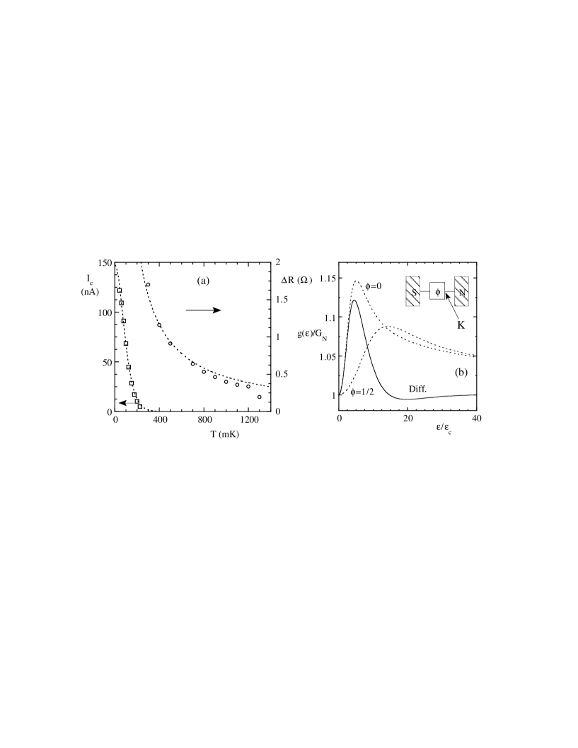
Fig.  5: (a) Left scale : Temperature dependence of the critical current derived from Fig. 4 data with a $25\Omega$ differential resistance criteria. Dashed line is a guide to the eye. Right scale : Temperature dependence of the amplitude of the magnetoresistance oscillations, Dashed line is a 1/T power-law fit. (b) Sketch of the spectral conductance as a function of the voltage bias in a loop-shaped sample with zero flux and half a flux quantum in the loop (dotted lines). The ratio distance S-K over distance S-N is 0.6. The full curve gives the difference of spectral conductance between these two cases. Inset shows the sample model. The arrow shows the point K where the pair amplitude is zero when the flux through the loop is $\varphi=\phi_{0}/2$.

4.3 Analysis of the oscillations amplitude

From the Fig. 4b, we observe that the magnetoresistance oscillations are very robust against the temperature. The oscillations at 1.3 K have an amplitude which is barely reduced as compared to the data at 0.7 K. Fig. 5 shows the temperature dependence of both the magnetoresistance oscillations amplitude and the Josephson critical current. The difference in behaviour is striking. While the critical current is exponentially suppressed at high temperature $T$, the magnetoresistance oscillations amplitude follows a $1/T$ power law. The deviation at high temperature is related to the closure of the gap near the superconducting transition of Al.

The $1/T$ power-law can be explained in a intuitive way, as discussed in the following. The magnetic flux in the loop creates interference between electron pairs travelling along one side of the loop or the other side. Let us consider the contribution of only one Al island. With two islands, the effects will add up.

Let us restrict to the two extreme cases of an integer or integer plus one half number of flux quantum in the loop. In the integer plus one half case, there is a destructive interference ($F=0$) of the diffusing pairs at the node K opposite to the S island, see Fig. 5b. In the integer case, the magnetic flux has no effect on the pair amplitude. In summary, the point K acts as an effective N reservoir when half a flux quantum threads the loop. This reduces the effective sample length from $L$ to a given fraction of $L$.

Fig. 5b shows the calculated spectral conductance in the two extreme cases $\varphi=0$ and $\varphi=\phi_{0}/2$. The difference between the two spectral conductances is restricted at low energy, since at point K, only electrons with an energy close to the Fermi level may remain coherent. The pairs with a large energy are unaffected by the flux, as their coherence length $L_{\epsilon}$ is much smaller than the loop perimeter. This makes the flux an unique tool for selecting the low-energy, long-range coherence in N-S structures with an Aharonov-Bohm loop.

Let us now estimate the impact of the interference on the sample conductance at finite temperature. We assume that the temperature $T$ is much larger than the Thouless temperature $\epsilon_{c}/k_{B}$. The effect of the interference is limited to an energy window of about $10\epsilon_{c}$, see Fig. 5b. In a first approximation, the spectral conductance enhancement (of about $15\%$) is cancelled for this population. The relative amplitude of the magnetoresistance oscillation is then given by $15\%$ of the ratio of this population ($10\,\epsilon_{c}$) over the thermal population ($\epsilon\leq k_{B}T$). This gives a ratio $1.5\,\epsilon_{c}/k_{B}T$.

This qualitative argument is confirmed by a rigourous calculation based on the Usadel equations [21]. A ratio of about $\epsilon_{c}/k_{B}T$ is in good agreement with the experiment. It has a natural interpretation, since it is the fraction $\epsilon_{c}$ of electrons from the thermal distribution $k_{B}T$ which remain coherent over the normal metal loop. The Thouless energy appears here again as the natural energy scale for the proximity superconductivity.

5 Conclusion and Perspectives

Although it used to appear as old-fashioned, the proximity effect has recently known a noticeable revival. This is due to the discovery of its natural mesoscopic status and the prodigeous progresses in nanofabrication. A major example is its natural length scale being the phase-breaking length of individual electrons $L_{\varphi}$. The proximity superconductivity in mesoscopic samples shows many unique features in the field of mesoscopic physics. It is an ensemble-averaged effect which affects at order 0 in $k_{F}l_{p}$ the electronic conductance of metallic samples [20]. The Thouless energy $\epsilon_{c}$ is the relevant energy scale for the proximity effect. This energy appears in the Josephson effect, the re-entrance effect, the density of states and the magneto-conductance oscillations. As an illustration, let us note that the Josephson coupling will appear in the S-N-S sample at the same temperature as the normal-state conductance would re-enter in the S-N-N sample.

Some experimental works have lead to discussions on the relevance of the theory, but up to now the theory has eventually explained the main experimental results. For instance, the resistance enhancement observed in some N-S structures [39] is now reliably understood as a 2D effect of redistribution of current lines as the temperature is decreased below the S metal superconducting transition [30, 40]. An open question consists of the interplay between the Andreev reflection and weak localization diagrams which could lead to the observation of $h/4e$-periodic oscillations of the magnetoresistance [34]. This effect has not been observed yet since the only observation of $h/4e$ periodicity [35] was in fact due to the tricky geometry of the samples [41].

One of the challenging perspectives in the field is the effect of interactions in the normal metal. This motivates the study of proximity effect in exotic materials like ferromagnetic metals [42].

6 Acknowledgements

We are grateful to P. Charlat who performed most of the experimental work on the re-entrance effect. We thank F. Wilhelm, F. Zhou, B. Spivak, T. Martin, A. Zaikin, and A. F. Volkov for illuminating discussions on the theory. We benefited of collaborations with M. Giroud and K. Hasselbach. We acknowledge financial support from Région Rhône-Alpes, D.R.E.T. and European Union through TMR contract FMRX-CT97-0143 ”Dynamics of Superconducting Nanocircuits”.

References

- [1] For a review, see Mesoscopic electron transport, ed. by L. L. Sohn, L. Kouwenhoven, and G. Schön, Kluwer Academic Publishers, Dordrecht, The Netherlands (1997).
- [2] Y. Imry, Introduction to Mesoscopic Physics, Oxford University Press, New York (1998).
- [3] B. Pannetier, J. Chaussy, and R. Rammal, Phys. Scripta T 13, 245, (1986).
- [4] P. Mohanty, E. M. Q. Jariwala, and R. A. Webb, Phys. Rev. Lett. 78, 3366 (1997).
- [5] R. A. Webb and S. Washburn, Rep. Prog. Phys. 55, 1311 (1992).
- [6] B. L. Ashuler, A. G. Aronov, and B. Z. Spivak, JETP Lett. 33, 94 (1981).
- [7] D. Y. Sharvin and Yu. V. Sharvin, JETP Lett. 34, 272 (1981), .
- [8] C. J. Lambert and R. Raimondi, J. Phys.: Condens. Matter 10, 901 (1998) and references therein.
- [9] C. W. J. Beenakker, Rev. Mod. Phys. 69, 731 (1997).
- [10] D. C. Ralph and V. Ambegaokar, Comments Cond. Mat. 18, 249 (1998).
- [11] H. Courtois, Ph. Gandit, and B. Pannetier, Phys. Rev. B 52, 1162 (1995); Phys. Rev. B 51, 9360 (1995).
- [12] F. K. Wilhelm, A. D. Zaikin, and G. Schön, J. of Low Temp. Phys. 106, 305 (1997)
- [13] A. F. Andreev, Sov. Phys. JETP 19, 1228 (1964).
- [14] H. A. Blom, A. Kadigrobov, A. M. Zagoskin, R. I. Shekhter, and M. Jonson, Phys. Rev. B 57, 9995 (1998).
- [15] P. G. de Gennes, Superconductivity of metals and alloys (Benjamin; N. Y.), 1964.
- [16] K. D. Usadel, Phys. Rev. Lett. 25, 507 (1970).
- [17] A. F. Volkov, A. V. Zaitsev, and T. M. Klapwijk, Physica C 210, 21 (1993); A. F. Volkov and A. V. Zaitsev, Phys. Rev. B 53, 9267 (1996); A. V. Zaitsev, JETP Lett. 51, 35 (1990).
- [18] Y. V. Nazarov and T. H. Stoof, Phys. Rev. Lett. 76, 823 (1996).
- [19] A. F. Volkov, N. Allsopp and C. J. Lambert, J. Phys. Condens. Matter 8, L45 (1996).
- [20] F. Zhou, B. Spivak, and A. Zyuzin, Phys. Rev. B 52, 4467 (1995).
- [21] A. A. Golubov, F. K. Wilhelm, and A. D. Zaikin, Phys. Rev. B 55, 1123 (1997).
- [22] S. Yip, Phys. Rev. B 52, 15504 (1995).
- [23] W. Belzig, F. K. Wilhelm, C. Bruder, G. Schön, and A. D. Zaikin, this volume.
- [24] P. Charlat, PhD thesis, Université Joseph Fourier, Grenoble, France (1996) ; H. Courtois, P. Charlat, Ph. Gandit, D. Mailly, and B. Pannetier, to be published.
- [25] S. Guéron, H. Pothier, N. O. Birge, D. Estève and M. H. Devoret, Phys. Rev. Lett. 77, 3025 (1996).
- [26] F. Zhou, P. Charlat, B. Spivak, and B. Pannetier, J. of Low Temp. Phys. 110, 841 (1998).
- [27] P. Visani, A. C. Mota, A. Pollini, Phys. Rev. Lett. 65, 1514 (1990).
- [28] C. W. J. Beenakker, Phys. Rev. B 46, 12841 (1992).
- [29] P. Charlat, H. Courtois, Ph. Gandit, D. Mailly, A. Volkov, and B. Pannetier, Phys. Rev. Lett. 79, 4950 (1996); Proceedings of the LT21 Conference, Czech. J. of Phys. 46, S6 3107 (1996).
- [30] F. K. Wilhelm, A. D. Zaikin and H. Courtois, Phys. Rev. Lett. 80, 4289 (1998).
- [31] V. T. Petrashov, R. Sh. Shaikhaidorov, P. Delsing, and T. Claeson, JETP Lett. 67, 513 (1998).
- [32] S. G. den Hartog, C. M. A. Kapteyn, B. J. van Wees, and T. M. Klapwijk, Phys. Rev. Lett. 76, 4592 (1996).
- [33] H. Courtois, Ph. Gandit, D. Mailly, and B. Pannetier, Phys. Rev. Lett. 76, 130 (1996).
- [34] B. Z. Spivak and D. E. Kmelnitskii, JETP Lett. 35, 412 (1982).
- [35] V. T. Petrashov, V. N. Antonov, P. Delsing, and T. Claeson, Phys. Rev. Lett. 70, 347 (1993).
- [36] A. Dimoulas, J. P. Heida, B. J. van Wees, T. M. Klapwijk, W. v. d. Graaf, and G. Borghs, Phys. Rev. Lett. 74, 602 (1995).
- [37] B.R. Patton, Proc. 13th Int. Conf. on Low Temp. Phys., 1972, Ed. by W.S. O’Sullivan, Plenum (New York).
- [38] J. Kutchinsky, R Taboryski, T. Clausen, C. B. Sørensen, A. Kristensen, P. E. Lindelof, J. Bindslev Hansen, C. Schelde Jacobsen, and J. L. Skov, Phys. Rev. Lett. 78, 931 (1997).
- [39] V. T. Petrashov, V. N. Antonov, P. Delsing, and T. Claeson, Phys. Rev. Lett. 74, 5268 (1995).
- [40] C. Lambert, R. Seviour, and A. F. Volkov, Phys. Rev. B. 58, 12338 (1998).
- [41] A. V. Zaitsev, Phys. Lett. A 194, 315 (1994).
- [42] M. Giroud, H. Courtois, K. Hasselbach, D. Mailly, and B. Pannetier, Phys. Rev. B. 58, R11872 (1998).