Temperature and magnetic-field dependence of the conductivity of YBa₂Cu₃O_7-δ films in the vicinity of superconducting transition: Effect of $T_{C}$-inhomogeneity

Abstract

Temperature and magnetic field dependences of the conductivity of YBa₂Cu₃O_7-δ films in the transition region are analyzed taking into account spatial inhomogeneity in transition temperature, $T_{c}$. (i) An expression for the superconducting contribution to conductivity, $\sigma_{s}(T,H,T_{c})$, of a homogeneous superconductor for low magnetic fields, $H\ll H_{c2}(0)$, is obtained using the solution of the Ginzburg-Landau equation in form of perturbation expansions [S.Ullah, A.T.Dorsey, Phys. Rev. B 44, 262 (1991)]. (ii) The error in $\sigma_{s}(T,H,T_{c})$ occurring due to the presence of $T_{c}$-inhomogeneity is calculated and plotted on an $H-T$ plane diagram. These calculations use an effective medium approximation and a Gaussian distribution of $T_{c}$. (iii) Measuring the temperature dependences of a voltage, induced by a focused electron beam, we determine spatial distributions of the critical temperature for YBa₂Cu₃O_7-δ microbridges with a 2 $\mu$m resolution. A typical $T_{c}$-distribution dispersion is found to be $\approx$1 K. For such dispersion, error in $\sigma_{s}(T,H,T_{c})$ due to $T_{c}$-inhomogeneity exceeds 30% for magnetic fields $H<1$ T and temperatures $|T-T_{c}|<0.5$ K . (iv) Experimental $R(T,H)$ dependences of resistance are well described by a numerical solution of a set of Kirchoff equations for the resistor network based on the measured spatial distributions of $T_{c}$ and the expression for $\sigma_{s}(T,H,T_{c})$.

I Introduction

The complicated crystal structure of high-$T_{c}$ superconductors (HTSC) leads to their substantial spatial inhomogeneity, which is especially important because of the very short coherence length, $\xi$. Inhomogeneities with spatial scale much larger than $\xi$ allow for an inhomogeneous distribution of the critical temperature, $T_{c}$, which affects properties of HTSC in the superconducting transition vicinity. As a result, it is often difficult to establish whether observed behavior of superconductors arise from intrinsic properties or from spatial inhomogeneity. This impedes analysis of experimental data in the transition region, which is often used to determine microscopic superconducting parameters and the mechanism of superconductivity.

The most obvious origin of $T_{c}$-inhomogeneity is variation in oxygen content over the sample. For YBa₂Cu₃O_7-δ (YBCO), $T_{c}$ is a relatively weak function of $\delta$ at $6.85<7-\delta<7$ (so called 90 K plateau) and falls abruptly at higher $\delta$.[2, 3] Even $\delta$ variations within the 90 K plateau can lead to $\approx$ 1 K variations in $T_{c}$. Meanwhile, experimental x-ray data show that $\delta$ variation can be substantially higher even for crystals exhibiting excellent transport properties.[4] Another origin of $T_{c}$-inhomogeneity is variation in cation (Y, Ba, Cu) composition. This origin can be dominant in thin YBCO films, as shown by simultaneous spatially resolved studies of cation composition and $T_{c}$ using electron probe microanalysis and low-temperature scanning electron microscopy (LTSEM), respectively.[5, 6] Elastic stresses around structural defects can also lead to $T_{c}$-inhomogeneity due to a strong pressure dependence of $T_{c}$ in HTSC compounds.[7] $T_{c}$ increase due to edge dislocations and low-angle grain boundaries was calculated to be $\sim 1$ K.[8] Spatial variations of the $c$-axis lattice parameter revealed by x-ray studies in YBCO films with almost uniform oxygen content also suggest stress-induced $T_{c}$-inhomogeneity.[9]

Presence of $T_{c}$-inhomogeneity manifests itself in various HTSC properties. Temperature dependence of the depinning current density in YBCO crystals implies that pinning sites are induced by spatial variations of $T_{c}$.[10] Systematic studies of YBCO crystal magnetization curves suggest the presence of local regions with reduced oxygen content, leading to the so called peak effect.[11, 12, 13] Meanwhile, $T_{c}$-inhomogeneity should have even greater impact on temperature dependences of transport coefficients just above the superconducting transition. This is confirmed by experimental data on conductivity, magnetoconductivity, and the Hall coefficient at temperatures $T\geq T_{c}+2$ K from Refs.[14, 15, 16] which were explained by assuming a Gaussian distribution of $T_{c}$ with dispersion in the range 0.6-2.3 K. However, these results can only serve as an indirect indication of the presence of $T_{c}$-inhomogeneity, due to a lack of experimental data about real $T_{c}$-distribution in the samples. Moreover, the temperature region in the vicinity of the superconducting transition, where $T_{c}$-inhomogeneity is especially important, was not considered.

A step forward has been made in Ref. [17] where resistor network calculations are used to analyse current density redistributions in $T_{c}$-inhomogeneous supercondictor in the transition region. It is shown that some anomalities in the temperature dependence of in-plane magnetoresistivity, such as negative magnetoresistivity excess, which are usually attributed to intrinsic effects can be quantitatively expalined by nonuniform $T_{c}$-distribution.

In the present work, we investigate the influence of $T_{c}$-inhomogeneity on properties of HTSC throughout the transition region and analyze experimentally determined spatial distributions of $T_{c}$ ($T_{c}$-maps). Measuring $T_{c}$-maps of YBCO films by LTSEM with 2 $\mu$m resolution, we reveal $\approx$ 1 K scatter of $T_{c}$ over the films. To calculate the effective conductivity of such an inhomogeneous material, one needs the expression for conductivity $\sigma(T,H,T_{c})$ of a uniform superconductor valid throughout the transition region. Such an expression was obtained in Ref. [18] by solving the time-dependent Ginzburg-Landau equation with Lawrence and Doniach Hamiltonian in the Hartree approximation.

It is well-known that magnetic field leads to a broadening of the superconducting transition which is roughly proportional to $\left(dH_{c2}/dT\right)^{-1}_{T=T_{c}}\approx 0.5$ K/T.[19] For fields $H>2$ T, this broadening dominates over inhomogeneous broadening due to scatter of local values of $T_{c}$. Therefore, we are interested in low fields, $H\leq 2$ T, where the influence of $T_{c}$-inhomogeneity is essential. Moreover, this range of magnetic fields is actual for most HTSC applications. Unfortunately, the final formula for conductivity obtained in Ref. [18] is only valid for high magnetic fields. In the present work, we deduce expressions for conductivity valid for low magnetic fields, $H\ll H_{c2}$, from the perturbation expansions in Ref. [18].

The present paper is organized as follows. In Sec. II the expression for the Cooper pair conductivity, $\sigma_{s}(T,H,T_{c})$, of a homogeneous superconductor is derived. In Sec. III we discuss methods to calculate the effective conductivity of an inhomogeneous superconductor. In Sec. IV the error in the value of $\sigma_{s}(T,H,T_{c})$ occurring due to the presence of $T_{c}$-inhomogeneity is calculated and the results are plotted on the $H-T$ plane diagram. Sec. V describes the samples and experimental techniques. In Sec. VI, measured spatial distributions of $T_{c}$ are analyzed and the broadening of the superconducting transition due to $T_{c}$-inhomogeneity is discussed. Finally, the experimental $R(T,H)$ dependences of resistance are interpreted on the basis of measured $T_{c}$-distributions and the expression for $\sigma_{s}(T,H,T_{c})$ derived in Sec. II.

II Conductivity of a homogeneous superconductor

To describe the temperature dependence of conductivity of a homogeneous superconductor throughout the transition region we employ the results obtained by Ullah and Dorsey.[18] They studied the time-dependent Ginzburg-Landau equation for anisotropic superconductor with the Hamiltonian introduced by Lawrence and Doniach[20] and an additional noise term. The magnetic field $H$ was assumed to be applied along the $c$-axis. Using the Hartree approximation Ullah and Dorsey obtained expressions for the transport coefficients which gave smooth interpolation between the high-temperature regime dominated by Gaussian fluctuations and low-temperature flux-flow regime. The expression for the Cooper pair conductivity in linear order to electric field was obtained in the form of two coupled perturbation expansions[18]:

$$\sigma_{s}=\sigma_{0}\sum_{n=0}^{N}(n+1)(A_{n}+A_{n+1}-2A_{n+1/2}),$$ (1)

where[21]

$$A_{n}=A_{n}(\tilde{\epsilon}_{H},h)=\left[(\tilde{\epsilon}_{H}+2hn)(1+d^{2}(\tilde{\epsilon}_{H}+2hn))\right]^{-1/2},$$ (2)

and

$$\epsilon_{H}=\tilde{\epsilon}_{H}-\Omega Th\sum_{n=0}^{N}A_{n}.$$ (3)

Here $h=H/H_{c2}(0)$, and $\epsilon_{H}$ is a field-dependent dimensionless temperature, $\epsilon_{H}=T/T_{c}-1+h$. Further,

$$\Omega=\frac{8\pi^{2}\left(2\kappa^{2}-1\right)\xi_{c}(0)k_{B}}{\gamma^{2}\phi_{0}^{2}},$$ (4)

$\xi_{ab}(0)$ and $\xi_{c}(0)$ are the correlation lengths in the CuO plane and transverse to it: $\xi_{ab}(0)=\hbar/\sqrt{2m_{ab}\alpha_{0}}$ (with similar relation for $\xi_{c}(0)$); $m_{ab}$ is the Cooper pair mass in CuO plane, $\alpha_{0}$ is related to the parameter $\alpha$ in Ginzburg-Landau Hamiltonian as $\alpha=\alpha_{0}\left(T/T_{c}-1\right)$, $d=s/2\xi_{c}(0)$, where $s$ denotes spacing between CuO planes, $\gamma=\xi_{c}(0)/\xi_{ab}(0)$ is an anisotropy parameter, $\phi_{0}$ is the flux quantum, $\kappa$ is the Ginzburg-Landau parameter, $H_{c2}(0)=\phi_{0}/2\pi\xi_{ab}^{2}(0)$, $N=1/h$, and $\sigma_{0}$ is a constant with dimensionality of a conductivity.

In order to avoid summation in the above expressions, the following approximation suggested in Ref. [18] is usually used. For high magnetic field ($\tilde{\epsilon}_{H}\ll 2h$) and 3D case ($d^{2}\tilde{\epsilon}_{H}\ll 1$) only terms containing $A_{0}$ are left in Eqs. (1) and (3) yielding $\sigma_{s}=\sigma_{0}/\sqrt{\tilde{\epsilon}_{H}}$ and $\epsilon_{H}=\tilde{\epsilon}_{H}-\Omega h/\sqrt{\tilde{\epsilon}_{H}}$ respectively. This leads to

$$\sigma_{s}=\frac{\sigma_{0}}{(\Omega Th)^{1/3}}\,\,{\cal F}\left[\frac{\epsilon_{H}}{\left(\Omega Th\right)^{2/3}}\right],$$ (5)

where function ${\cal F}(x)$ satisfies cubic equation,

$$x{\cal F}^{2}=1-{\cal F}^{3}.$$ (6)

The solution of this equation can be written down as

$${\cal F}(x) = \theta+x^{2}/(9\theta)-x/3,$$ (7)

$$\theta = \left(1/2-x^{3}/27+\sqrt{(27-4x^{3})/108}\right)^{1/3}.$$ (8)

The function ${\cal F}(x)$ is equivalent to the function $F_{3D}$ in Ref. [18] though expressions (6) and (8) for this function are not presented there.

Despite Eq. (5) is widely used, its applicability range needs a special discussion. Indeed, since the series (3) are diverging, omitting all terms except the first one is hardly permissible. At least, it is obviously incorrect if the condition $\tilde{\epsilon}_{H}\ll 2h$  does not hold. Hence, for magnetic fields we deal with, $H<2$ T, the high-field approximation of Ref. [18] is not valid except for the low-temperature part of the superconducting transition. As argued in Ref. [18], Eq. 5 can also be considered as a scaling relation with unknown scaling function ${\cal F}$ and then it is valid in a wider range of magnetic fields. However, simple numerical calculations show that, e. g., for YBa₂Cu₃O_7-δ, the scaling does not work for fields $H<2$ T. Therefore, we derive new, low-field approximation for conductivity from Eqs. (1) and (3). For $h\ll 1$ one can replace summation for $n\geq 1$ by integration using Euler-Maklaurin formula[22] and obtain the following analytical expressions for conductivity:

$$\sigma_{s}/\sigma_{0} = A_{0}-2A_{1/2}+\frac{9}{4}A_{1}-2A_{3/2}+A_{2}$$ (10)

$$-{3+8d^{2}\over 4(2+4d^{2})^{3/2}}+{3h\over 8}(1+2d^{2}(\tilde{\epsilon}_{H}+2h))A_{1}^{3},$$

$$\epsilon_{H} = \tilde{\epsilon}_{H}-\frac{\Omega T}{2}\left(2hA_{0}+hA_{1}+{h\over\sqrt{2(1+2d^{2})}}\right.$$ (12)

$$\left.+{1\over d}\ln\left({d+4d^{3}+2d^{2}\sqrt{2+4d^{2}}\over 2d^{3}\tilde{\epsilon}_{H}+d+2d^{2}/A_{1}}\right)\right)$$

Equations (10) and (12) present non-explicit dependence of conductivity for a homogeneous superconductor on temperature and magnetic field. They are derived without any assumptions about 3D or 2D character of superconductivity and therefore applicable for arbitrary anisotropy parameter. These equations are used below for calculations presented in Sec. III and V.

Under conditions

$$\tilde{\epsilon}_{H},h\ll 1/d^{2}\ll 1$$ (13)

equations (10) and (12) can be substantially simplified yielding an explicit expression for the Cooper pair conductivity:

$$\frac{\sigma_{s}}{\sigma_{0}}={1\over\sqrt{\tilde{\epsilon}_{H}}}-{2\over\sqrt{\tilde{\epsilon}_{H}+h}}+{1\over\sqrt{\tilde{\epsilon}_{H}+2h}}+{7h+2\tilde{\epsilon}_{H}\over 8(\tilde{\epsilon}_{H}+2h)^{3/2}}$$ (14)

$$\tilde{\epsilon}_{H} = (\Omega Th)^{2/3}\,\,{\cal F}^{-2}\left[\frac{(1+\Lambda)\ T/T_{c}-1+h}{(\Omega Th)^{2/3}}\right],$$ (15)

$$\Lambda = \Omega T_{c}\ \frac{\ln 8d^{2}}{2d},$$ (16)

where ${\cal F}$ is the function defined by Eqs. (6) or (8). Another advantage of these equations is that the conductivity depends on $d$ only through parameter $\Lambda$ which characterizes the shift of the apparent transition temperature with respect to $T_{c}$. This shift is always present in the Hartree approximation as a result of renormalization of the parameter $\alpha$ in the Ginzburg-Landau Hamiltonian.

Eqs.(10) and (12) as well as Eqs.(14) and (16) defining temperature and magnetic field dependence of conductivity contain only two key parameters: $d$ and $\Omega$. Parameter $d$ depends on the value of coherence length $\xi_{c}(0)$ which is not known well. An accurate determination of $\xi_{c}(0)$ is difficult because of bilayered structure of the YBCO unit cell. A systematic analysis performed in Ref. [23] shows that a good approximation for YBCO is the assumption of equally spaced CuO layers with interlayer distance $s=6\ \AA$. Then, a simultaneous fitting of conductivity, magnetoconductivity and susceptibility data gives $\xi_{c}(0)=1.2\AA$ leading to $d=2.5$.[23] This value does not contradict to results of other works[24, 25, 28] assuming the distance between superconducting layers $s\approx 11.7\ \AA$. They give values of $\xi_{c}(0)$ in the range between 1.3 and 3 $\AA$ which corresponds to $1.9<d<4.5$. Obviously, this uncertainty in $d$ is very large. Fortunately, it is not so important in the range of $H$ and $T$ that we consider. Indeed, for YBCO the conditions (13) are satisfied within several kelvins around the transition unless the magnetic field is very high. Then, as follows from Eqs. (14) and (16),

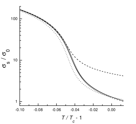
FIG. 1.: Temperature dependence of Cooper pair conductivity for YBCO in magnetic field $H=2$ T. Symbols show the exact result of UD model,[18] Eqs. (1), and (3); dashed line is the high-field approximation proposed by Ullah and Dorsey, Eqs. (5) and (8) (shifted along $x$-axis by $-\Lambda$); solid line is the low-field approximation proposed in the present paper, Eqs. (10) and (12); dotted line is an approximate explicit expression for low fields given by Eqs. (14) and (16).

change in $d$ leads only to a shift of apparent transition temperature but does not affect the shape of the transition curve. The second parameter $\Omega$ depends on the coherence length $\xi_{ab}(0)$ and the Ginzburg-Landau parameter $\kappa$. The former was also taken from Ref. [23], $\xi_{ab}=11\ \AA$. Meanwhile, it is quite difficult to find in literature an accurate estimate for $\kappa$. We used the value $\kappa=30$ providing the best fit to our experimental data for YBCO films. Then, from equation (4) one obtains $\Omega=5\times 10^{-4}$.

Figure 1 presents comparison of the temperature dependences of Cooper pair conductivity given by straightforward summation in (1) and (3), and by two analytical approximations: high-field approximation, Eqs. (5) and (8), proposed by Ullah and Dorsey and low-field approximation, Eqs. (10) and (12), suggested in the present work. An approximate explicit expression for low fields given by Eqs. (14) and (16) is also shown as dotted line. For $H=2$ T which is the case shown in the figure, the low-field approximation is far more accurate than the high-field one. For lower magnetic fields the deviation between the result of exact summation and the low-field approximation is almost indistinguishable. By contrast, the high-field approximation fails for temperatures $T\gg T_{c}$ where it four times overestimates the result of exact summation which is $\sigma=\sigma_{0}/(4\sqrt{\epsilon_{H}})$.

Figure clearly shows that the apparent transition temperature is shifted downward from $T_{c}$. For given set of parameters the dimensionless shift is $\Lambda\approx 0.03$. In order to avoid confusion, the data in all figures below are shifted along $x$-axis so that $T_{c}$ corresponds to the apparent transition temperature. It should be also noted that the shift $\Lambda$ does not enter the high-field approximation suggested by Ullah and Dorsey, Eqs. (5) and (8). This approximation predicts transition at $T=T_{c}$ in contradiction to basic equations of UD model, Eqs. (1) and (3). In order to make the high-field approximation merge all other curves in Fig. 1 at least at low $T$, we had to shift the corresponding dashed curve on the value $\Lambda$ “by hand”.

The constant $\sigma_{0}$ entering UD model depends on a phenomenological quantity, the relaxation rate of the order parameter. It is natural to estimate $\sigma_{0}$ using well-known Aslamazov-Larkin result[26] for high-temperature asymptotic in 3D case: $\sigma_{s}^{3D}={e^{2}}/{32\hbar\xi(0)\sqrt{\epsilon_{H}}}$. Thus, we have

$$\sigma_{0}=e^{2}/\,8\hbar\xi(0)$$ (17)

Let us now discuss the applicability range for the results obtained in this Section. The indirect (Maki-Thompson) contribution to the order parameter fluctuations [27] is not taken into account in the UD model. However, there are grounds to believe that neglecting Maki-Thompson term would not affect the results obtained in the transition region (few Kelvins around $T_{c}$) since the direct Aslamazov-Larkin process is dominant over the indirect one in this temperature range.[28] One should also keep in mind that the UD model does not take into account vortex pinning and predicts flux-flow behavior in the limit of low temperatures. Therefore, it cannot be used at temperatures well below $T_{c}$, where the current-voltage characteristics are nonlinear.

III Account of $T_{c}$-inhomogeneity

Let us now consider how the properties of a superconductor can be affected by spatially inhomogeneous distribution of critical temperature. First, we suppose that the correlation length $r_{c}$ of $T_{c}$-distribution is so large that the temperature region near $T_{c}$ where $\xi(T)>r_{c}$ can be ignored. This assumption seems to be quite reasonable since the coherence length of HTSC is much smaller than $r_{c}$ obtained from LTSEM data, see Tab. 1. The condition $r_{c}\gg\xi$ makes it possible to ignore the correlation between the superconducting order parameter in adjacent fragments and to consider them independently. Therefore, the expression for the conductivity obtained in the previous section for a homogeneous superconductor can be used to describe local conductivity $\sigma(T,H,T_{c})$ of a homogeneous fragment with given $T_{c}$.

The straightforward way to determine the conductivity $\sigma^{\rm inh}(T,H)$ of a $T_{c}$-inhomogeneous superconductor is to start from the spatial distribution of $T_{c}$ over the sample. The value of $\sigma^{\rm inh}(T,H)$ can be determined exactly from the values of local conductivities $\sigma(T,H,T_{c})$. In this work we determined the spatial distributions of the critical temperature in YBCO films using LTSEM (see Sec. V). This method, however, leads to the lack of information about small-scale inhomogeneities with $r_{c}\leq r_{\exp}$, where $r_{\exp}$ is the spatial resolution of the technique. Therefore, if small-scale inhomogeneity is essential, or if spatial distribution of $T_{c}$ is unknown, a Gaussian $T_{c}$-distribution function together with, e. g., effective medium approach can be used to find $\sigma^{\rm inh}(T,H)$.

The problem of conductivity of an inhomogeneous medium has the exact analytical solution only for a special case of symmetric distribution of phases in 2D system.[29] In the general case one has to use some approximation. According to the effective medium approach[30] (EMA), the conductivity $\sigma^{\rm inh}(T,H)$ is given by the solution of the equation

$$\int\frac{\sigma^{\rm inh}(T,H)-\sigma(T,H,T_{c})}{(D-1)\,\sigma^{\rm inh}(T,H)+\sigma(T,H,T_{c})}f(T_{c})dT_{c}=0,$$ (18)

where $D$ is the dimensionality of the system. Here $f(T_{c})$ is a distribution function of critical temperature over the sample which shows the relative volume occupied by fragments with given $T_{c}$. Despite the apparent simplicity, EMA gives rather high accuracy (up to few percents) unless the system is in the very vicinity of the percolation threshold.[31] In the case of thin film samples with thickness less than the correlation length of $T_{c}$-inhomogeneity, $r_{c}$, EMA expression (18) with dimensionality $D$=2 should be used. It should be emphasized that this dimensionality has nothing to do with the dimensionality of the superconducting properties mentioned in relation with formula (5); the first one depends on the geometry of the sample, while the latter is associated with anisotropy of the crystal structure.

IV $H-T$ diagrams

In this section we estimate the effect of $T_{c}$-inhomogeneity on the apparent value of the Cooper pair conductivity in the vicinity of the superconducting transition. Usually, experimental data on $\sigma(T,H)$-dependences in the transition region are studied first by subtracting the conductivity of normal electrons, $\sigma_{n}$, and then analyzing the remaining conductivity of Cooper pairs, $\sigma_{s}$. In the case of inhomogeneous sample such procedure would lead to an error in $\sigma_{s}$: its apparent value determined from experimental data would be different from that for a homogeneous superconductor. To quantitatively estimate this error we consider two samples: uniform, with critical temperature $T_{c0}$, and inhomogeneous one with a Gaussian distribution of critical temperatures with average $T_{c0}$ and dispersion $\delta T_{c}$:

$$f(T_{c})={1\over\sqrt{2\pi}\,\delta T_{c}}\exp\left(-\frac{\left(T_{c}-T_{c0}\right)^{2}}{2\,\delta T_{c}^{2}}\right).$$ (19)

Now two quantities, $\sigma_{s}^{\rm{hom}}(T,H)$ and $\sigma_{s}^{\rm{inh}}(T,H)$ can be compared. $\sigma_{s}^{\rm{hom}}$ is the Cooper pair conductivity for homogeneous sample given by the expressions (10) and (12) obtained on the basis of UD model. The conductivity $\sigma^{\rm{inh}}$ of the inhomogeneous sample is determined by EMA formula (18) with $f(T_{c})$ being Gaussian distribution function (19), and local conductivities defined as sum of the superconducting, $\sigma_{s}^{\rm{hom}}$, and normal, $\sigma_{n}$, contributions. Then, one should subtract the normal contribution from $\sigma^{\rm{inh}}$ and obtain the apparent superconducting contribution to conductivity for the inhomogeneous sample:

$$\sigma_{s}^{\rm{inh}}(T,H)=\sigma^{\rm{inh}}(T,H)-\sigma_{n}(T,H).$$ (20)

Further, to proceed with calculations some assumptions are needed about the temperature and magnetic field dependences of $\sigma_{n}$. We neglect the magnetoresistance of HTSC in the normal state which is very small and use a linear approximation for the temperature dependence of the resistivity:

$$\sigma_{n}(T,H)=\sigma_{n}(T,0)=1/\left(C_{1}+C_{2}T\right).$$ (21)

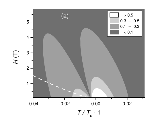
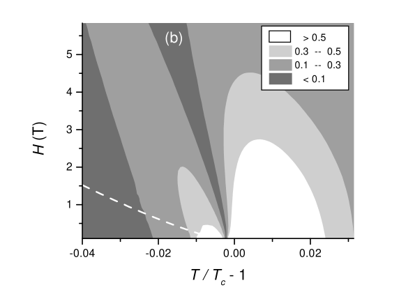
FIG. 2.: Diagrams in the “magnetic field”—“temperature” plane illustrating the effect of $T_{c}$-inhomogeneity on the apparent value of Cooper pair conductivity, $\sigma_{s}$. Absolute values of the reduced difference of (a) conductivities $|\sigma_{s}^{\rm{inh}}/\sigma_{s}^{\rm{hom}}-1|$ and (b) magnetoconductivities $|\left(\sigma_{s}^{\rm{inh}}\right)_{H}^{\prime}/\left(\sigma_{s}^{\rm{hom}}\right)_{H}^{\prime}-1|$ for homogeneous and inhomogeneous superconductors are shown. Calculations are based on Eqs. (10) and (12). For inhomogeneous superconductor, the calculations use an effective medium approach, Eq. (18), and a Gaussian distribution of $T_{c}$ with dispersion $\delta T_{c}=1$ K. Brighter regions correspond to a stronger influence of $T_{c}$-inhomogeneity. The influence is maximal in low magnetic fields and in the vicinity of $T_{c}$. Presented results are not valid below the white dashed lines which correspond to the melting transition of vortex lattice (the data are taken from Refs. [32, 33]).

The key parameter for calculations is the dispersion of Gaussian $T_{c}$-distribution (19), $\delta T_{c}$. We used the value $\delta T_{c}=1$ K which is approximately the average dispersion for studied YBCO films determined from their $T_{c}$-maps. The values for $\Omega$ and $d$ were the same as in Sec. II, other parameters were: $C_{1}$=1.06 $\mu\Omega$m, $C_{2}$=0.0035 $\mu\Omega$m/K (see Tab. 1), $T_{c}$=90 K, $D$=2. We also assume that the inhomogeneity of a superconductor manifests itself in inhomogeneity of the critical temperature only, while all the other superconducting parameters and the normal state conductivity are supposed to be uniform.

It is convenient to consider $H$–$T$ diagram which shows the absolute value of the relative difference: $|\sigma_{s}^{\rm{inh}}/\sigma_{s}^{\rm{hom}}-1|$, see Fig. 2a. The effect of $T_{c}$-inhomogeneity on the magnetoconductivity is illustrated by Fig. 2b showing the same diagram for the quantity $|\left(\sigma_{s}^{\rm{inh}}\right)_{H}^{\prime}/\left(\sigma_{s}^{\rm{hom}}\right)_{H}^{\prime}-1|$, where $(\sigma_{s})^{\prime}_{H}$ denotes partial derivative of conductivity with respect to magnetic field. Brighter regions on the diagrams correspond to larger values, i.e., to stronger influence of $T_{c}$-inhomogeneity on the values of $\sigma_{s}$ and $(\sigma_{s})_{H}^{\prime}$. The influence becomes crucial in a $1$ K–wide region around $T_{c}$ and for magnetic fields $H<0.5$ T where ignoring $T_{c}$-inhomogeneity would lead to $\sim 50\%$ error in $\sigma_{s}$. The following conclusions can be drawn from the diagrams:

(i) $T_{c}$-inhomogeneity plays greater role in the very vicinity of the transition; far from the transition the difference in local $T_{c}$’s is small compared to $|T-T_{c}|$ and, hence, not so important.

(ii) $T_{c}$-inhomogeneity plays greater role in low magnetic fields. The application of magnetic field leads to a broadening of the transition even in a homogeneous superconductor. Since for most HTSC  $dH_{c2}/dT\approx-2$ T/K at  $T=T_{c}$,[19] one can roughly estimate the increase in the transition width as one degree for $H$ increase of 2 T. Therefore, for fields $H>2$ T the dispersion in critical temperatures $\delta T_{c}\approx 1$ K is masked by $H$-induced broadening of the transition.

(iii) $T_{c}$-inhomogeneity has greater effect on the magnetoconductivity of a superconductor than on its conductivity. From practical point of view it is often preferable to analyze experimental data on magnetoconductivity rather than on conductivity. This is because the contribution of normal electrons to magnetoconductivity is negligible in the vicinity of $T_{c}$, while the analysis of conductivity data always requires account of the normal conductivity and, hence, additional assumptions about its temperature dependence. However, as follows from the diagrams, the analysis of magnetoconductivity data needs more careful account of $T_{c}$-inhomogeneity. The reason for that, as was earlier noted by Lang et al.,[16] lies in the stronger dependence of magnetoconductivity on $T_{c}$, e.g., for high temperatures, $T\gg T_{c}$, one has $\sigma_{s}\propto\left(T-T_{c}\right)^{-1/2}$, while $\partial\sigma_{s}/\partial H\propto\left(T-T_{c}\right)^{-3/2}$.

The dashed line in Fig. 2 corresponds to the melting transition of the Abrikosov vortex lattice as determined from experiments on YBCO crystals. [32, 33] It is remarkable that different methods, neutron small angle scattering,[32] as well as magnetization and transport measurements,[33] yield the same position of the melting line. We believe that it can serve as a rough estimate of the applicability range of the UD model. Below this line, our results obtained on the basis of the UD model are not valid.

V Samples and Experimental details

YBa₂Cu₃O_7-δ films with thickness of 0.2 $\mu$m were grown by dc magnetron sputtering on NdGaO₃, AlLaO₃ and MgO substrata. The details of the procedure are described elsewhere.[9] X-ray data have shown the presence of only (00l) reflexes confirming $c$-orientation of the films. The Raman spectroscopy analysis has revealed their high epitaxiality. Microbridges of 500$\times$50 $\mu$m size were formed by a standard photolithography. Six samples were investigated; some important parameters are presented in Tab. 1.

The temperature dependences of the resistivity were measured at driving current 1 mA and magnetic fields $H$=0, 0.3, 0.6, 0.9 T  applied along the $c$-axis. Measurements were done inside a temperature stabilized Oxford He flow cryostat (model CF-1200) under helium atmosphere, using the standard four-probe dc method, a Keithly 220 programmable current source and a Keithly 182 sensitive digital voltmeter. Contacts to the samples were made by thin gold wires attached to the sample surface by silver paste. The temperature inside the cryostat was controlled and stabilized by an Oxford programmable temperature controller ITC4 with accuracy up to 0.01 K. The temperature of the sample was measured by copper-constantan thermocouple; voltage was read by a DMM5000 integrating digital multimeter. The measurement was started when the sample was in the normal state (at least 40 K above $T_{c}$) and performed during a slow cooling procedure down to zero resistivity of the sample. Then the sample was heated and the measurement was repeated at another value of magnetic field. The accuracy of the voltage measurements was about 10 nV.

The LTSEM measurements were carried out with an automated scanning electron microscope CamScan Series 4-88 DV100. The microscope is equipped with a cooling sample stage, its temperature can be lowered down to 77 K using an Oxford N flow cryostat. The temperature is maintained in the range 77-350 K With accuracy up to 0.1 K by a temperature controller ITC4. The bias current was varied from 0.2 to 2.0 mA so that its value was large enough to detect electron beam induced voltage (EBIV) and small enough to avoid distortion of the superconducting transition. EBIV was measured using the standard four-probe method. A precision instrumentation amplifier incorporated into the microscope chamber was used to increase the signal-to-noise ratio. To extract the local EBIV signal, lock-in detection was used with a beam-modulation frequency of 1 kHz. The electron beam current was 10^-8 A, while the acceleration voltage was 10 kV.

The method for determination of the spatial distribution of critical temperature is based on LTSEM technique[36, 37] and is described in detail in Ref. [38]. Heating by electron beam elevates the temperature locally by $\delta T_{\rm{heat}}\leq 1$ K causing a change, $\delta\rho$, in the local resistivity. As a result, a change in the voltage, EBIV, occurs across the sample biased by a constant transport current. Temperature dependence of EBIV has the maximum at some temperature, $T_{m}$, corresponding to the maximum in $\delta\rho$. Thus, the local transition temperature can be determined as $T_{c}=T_{m}+\delta T_{\rm{heat}}/2$. Scanning the electron beam over the film allows us to determine the spatial distribution of $T_{c}$. In order to remove the distorting effects associated with thermal diffusion into adjacent regions of the film a numerical deconvolution method was used. Figure 3 shows temperature dependences of EBIV for two adjacent regions of sample 1 before and after the deconvolution procedure. After the deconvolution, both dependences have a pronounced major peak; its position defines the local $T_{c}$. It follows from Fig. 3 that the difference in $T_{c}$ for two regions separated by 5 $\mu$m can be as large as 0.7 K. The method allows the spatial resolution of 2 $\mu$m and the temperature resolution of 0.2 K. The $T_{c}$-map for sample 1 is shown in Fig. 4. After $T_{c}$-map is determined, one can easily calculate distribution function $f(T_{c})$ defining the relative volume occupied by fragments with given $T_{c}$; $f(T_{c})$ for sample 1 is shown in Fig. 5.

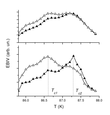
FIG. 3.: Temperature dependences of electron beam induced voltage measured by LTSEM for two regions of sample 1 separated by 5 $\mu$m distance. The upper panel shows raw signals, the lower panel shows the same dependences after deconvolution procedure. Local values of the critical temperature, $T_{c1}$ and $T_{c2}$, are determined by positions of the peaks.

Further, using $T_{c}$-map and the expression for conductivity $\sigma(T,H,T_{c})$ of a $T_{c}$-uniform fragment, one can calculate the spatial distribution of current density in the superconductor. First, the film is approximated by a square network of resistors. Then, the set of Kirchoff equations is solved with respect to electric potentials in the nodes of the network. For this purpose an iterative procedure with overrelaxation method is used with fixed potentials of the two opposite sides of the network.[31] As

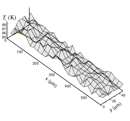
FIG. 4.: Spatial distribution of critical temperature in sample 1 determined from LTSEM data. Distribution is smoothed with respect to the initial one measured with 2 $\mu$m resolution.

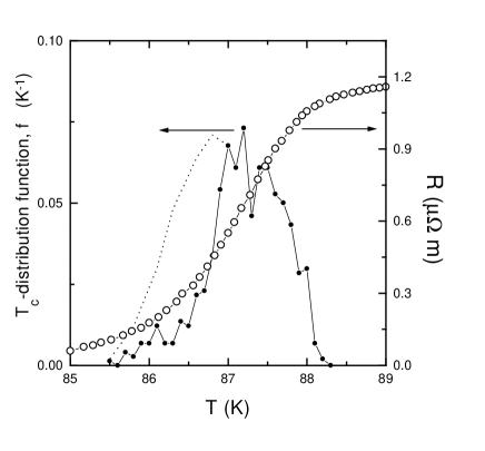
FIG. 5.: Experimental temperature dependence of resistivity (circles) for $H=0$ and the distribution function, $f(T_{c})$, of critical temperature (solid line) determined from $T_{c}$-map shown in Fig. 4. All the data are for sample 1. The dotted line shows a plausible shape of the total distribution function.

a result, the current density distribution as well as the total resistance of the superconductor are calculated for any temperature in the vicinity of the superconducting transition.

As the temperature is lowered, the current density distribution becomes noticeably inhomogeneous. As a result, some normal-conducting regions of the film are shunted by surrounding superconducting regions. $T_{c}$ of these shunted regions cannot be measured by the present method. However, one can expect that ambiguity in their $T_{c}$’s would not lead to substantial errors in results of resistor network calculations. Indeed, in the high-temperature part of the superconducting transition, the conductivity of these regions is known since they are in the normal state, while at lower temperatures they are off the main current path and make a minor contribution to the film resistance. Figure 5 represents distribution function $f(T_{c})$ determined from the $T_{c}$-map. The dotted line in the same figure shows a plausible shape of the total distribution function.

When the spatial distribution of critical temperature $T_{c}({\bf r})$ is given, one can estimate the correlation length of $T_{c}$-inhomogeneity. It is defined from the correlation function $G(r)$ of $T_{c}$-distribution :

$$G(r)=\frac{\overline{T_{c}({\bf R}+{\bf r})T_{c}({\bf R})}-\overline{T_{c}}^{2}}{\overline{T_{c}^{2}}-\overline{T_{c}}^{2}},$$ (22)

where averaging is performed over all R and all directions of r within the bridge. The value $G=1$ corresponds to full correlation and $G=0$ to the absence of correlation. For most samples the correlation function fits very well the exponential decay, $G(r)\propto e^{-r/r_{c}}$.

VI Experimental results

The parameters of studied YBCO films are presented in Tab. 1. The fourth column shows the width, $\Delta T_{R}$, of resistive transition defined as the doubled dispersion of the Gaussian fitting $dR/dT$ peak for $H=0$. The value $\Delta T_{R}$ equals to approximately 0.8 of the transition width defined by 10%-90% level of normal resistance.

The width $\Delta T_{c}$ of the experimentally determined distribution function $f(T_{c})$ was calculated by the same procedure as $\Delta T_{R}$. For samples marked by (^∗) the distribution function had two rather than one peak. In this case we calculated $\Delta T_{c}$ as a mean-squared deviation:

$$\Delta T_{c}=2\sqrt{\left\langle(T_{c}-\bar{T_{c}})^{2}\right\rangle}$$ (23)

where the averaging is performed over the area under the double-peak Gaussian fitting $f(T_{c})$. Application of Eq. (23) to the distribution function itself is less reliable because the value of $\Delta T_{c}$ is strongly affected by the tails of the distribution.

Further, we assume that the total broadening of the transition is caused by summation of homogeneous and inhomogeneous broadening and the simple relation can be written:

$$\Delta T_{R}^{2}=\Delta T_{\rm{hom}}^{2}+\Delta T_{c}^{2},$$ (24)

where $\Delta T_{\rm{hom}}$ is the homogeneous broadening of the transition.

The scale $r_{c}$ of $T_{c}$-inhomogeneity was determined by fitting the correlation function $G(r)$, Eq. (22), with an exponential decay, $\exp(-r/r_{c})$. Values of $r_{c}$ vary much for different samples and depend primarily on the substrate. This is consistent with results of x-ray studies which revealed clusters of dislocations of $\sim$80 $\mu$m size in MgO substrate used for sample 1. By contrast, sample 4 grown on NdGaO₃ substrate was of higher quality and no large-scale clusters in the substrate were observed. It should be noted, that values of $r_{c}$ in Table 1 can overestimate the true correlation length of $T_{c}$-inhomogeneity especially for samples with small $r_{c}$. The reason is that $r_{c}$ is always larger than the resolution of the experimental method, $r_{\exp}=2$ $\mu$m. Presence of $T_{c}$-inhomogeneity on small scales can be revealed by x-ray diffraction studies.

Table 1. Some characteristics of studied YBCO thin film samples. The transition width, $\Delta T_{R}$, is defined by the width of $dR/dT$ peak; $\Delta T_{c}$ is the dispersion of $T_{c}$- distribution; $\Delta T_{\rm{hom}}$ is the intrinsic broadening of the transition; $\Delta T_{\rm{EBIV}}$ is the average width of the local temperature dependence of EBIV; $r_{c}$ is the correlation length of $T_{c}$-distribution; $\rho_{n}(T)$ is the linear fit for the temperature dependence of resistivity in the 150-300 K range.

No.	Substrate	$T_{c}$, K	$\Delta T_{R}$, K	$\Delta T_{c}$, K	$\Delta T_{\rm{hom}}=$	$\Delta T_{\rm{EBIV}}$, K	$r_{c}$, $\mu$m	$\rho_{n}$($T$, K), $\mu\Omega\,m$
					$\sqrt{\Delta T_{R}^{2}-\Delta T_{c}^{2}}$
1	MgO	86	1.5	1.2	1.1	1.1	80	1.06+0.0035 $T$
2	AlLaO3	92.8	0.4	0.3	0.3	0.3	-	0.14+0.003 $T$
3	AlLaO3	91.5	1.7	0.8∗	1.5	0.9	45	-
4	NdGaO3	89	1.5	0.2	1.5	0.9	6	1.21+ 0.02 $T$
5	NdGaO3	88.5	1.9	0.3	1.9	1.7	16	1.26+0.018 $T$
6	NdGaO3	87	1.7	0.8∗	1.5	0.5	33	0.96+0.0045 $T$

The size of the area where the coherent scattering of x-ray wave is established has been found to be 30-100$\AA$ for YBCO films.[9, 34] This value defines the lower limit for $r_{c}$. It is in agreement with the value $r_{c}\approx 30~{}\AA$ for the size of $T_{c}$-uniform fragment in YBCO film deduced from analysis of experimental data on voltage noise in the superconducting transition region.[35]

The seventh column, $\Delta T_{\rm{EBIV}}$, shows the average width of the local temperature dependence of the EBIV which should be closely related to the homogeneous broadening $\Delta T_{\rm{hom}}$. Indeed, a good agreement is observed for samples 1, 2 and 5. In the case of samples 3 and 6 a specific shape of distribution function $f(T_{c})$ which invalidates simple relation (24) can be responsible for the deviation. For sample 4 this deviation is probably related to very short correlation length $r_{c}$. The last column in Tab. 1 represents the linear fit for the temperature dependence of resistivity in the 150-300 K range; the error in determination of the fit coefficients is 0.2–1%.

As follows from Tab. 1, inhomogeneous broadening, $\Delta T_{c}$, of the resistive transition is of the same order as homogeneous one, $\Delta T_{\rm{hom}}$. The homogeneous broadening characterizes the transition width for a fragment of superconducting film of 2 $\mu$m size. This width can be either an intrinsic property of a homogeneous superconductor or it can be associated with $T_{c}$-inhomogeneity on scales $<2~{}\mu$m. Large scatter of $\Delta T_{\rm{hom}}$ in Tab. 1 suggests the presence of small-scale $T_{c}$-inhomogeneity at least in the samples with large $\Delta T_{\rm{hom}}$.

Let us now examine the effect of $T_{c}$-inhomogeneity on the experimental temperature dependences of conductivity. Data for samples 1 and 4 with maximal and minimal $r_{c}$ will be analyzed. In order to extract the superconducting contribution, $\sigma_{s}(T,H)$, to conductivity from the measured resistance $R(T,H)$ we use Eq. (21) and data from Tab. 1. The extracted temperature dependences of $\sigma_{s}$ were fitted by two models: for homogeneous and for $T_{c}$-inhomogeneous superconductor. For homogeneous superconductor they were fitted directly by low-field approximation, Eqs. (10) and (12), derived in Sec. II. The parameters $\sigma_{0}$, $\kappa$ and $T_{c}$ were free. For $T_{c}$-inhomogeneous superconductor the same formulas were used to calculate conductivities of local fragments with uniform $T_{c}$. Effective conductivity $\sigma_{s}(T,H)$ of the whole sample was calculated by solving resistor networks based on the measured $T_{c}$-maps. This method has only two fitting parameters: $\sigma_{0}$ and $\kappa$. Theoretical estimate for $\sigma_{0}$ was obtained in Sec. II by comparison of the results of UD model at high temperatures and Aslamazov-Larkin formula. However, because of sample imperfections and a large error in determination of the sample thickness, $\sigma_{0}$ should be a free parameter. For studied samples $\sigma_{0}$ differs from the value given by Eq. (17) by a factor between 0.6 to 1.5. As follows from formulas of Sec. II, $\sigma_{0}$ controls the magnitude of the Cooper pair conductivity, while $\kappa$ determines the width of the resistive transition.

The experimental dependences $\sigma_{s}(T)$ for sample 1 for three magnetic fields and their fits by the “inhomogeneous” model are presented in Fig. 6. The dashed line shows the fit by the “homogeneous” model for $H=0.6$ T.

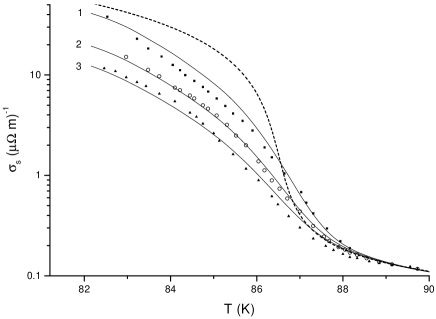
FIG. 6.: Experimental temperature dependences (symbols) of superconducting contribution to conductivity, $\sigma_{s}$, for sample 1 and their fits (solid lines) calculated by solving resistor networks based on the measured spatial distribution of $T_{c}$ and Eqs. (10) and (12)for three magnetic fields: (1) $H=0.3$ T, (2) $H=0.6$ T, (3) $H=0.9$ T; the fitting parameter is $\kappa=50$. The dashed line shows fit for a homogeneous superconductor, Eqs. (10) and (12), for $H=0.6$ T with fitting parameters $T_{c}=87.1$ K and $\kappa=30$. Fits taking account of $T_{c}$-inhomogeneity are in a much better agreement with experiment.

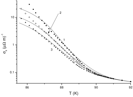
FIG. 7.: Experimental temperature dependences (symbols) of superconducting contribution to conductivity, $\sigma_{s}$, for sample 4 and their fits (lines) based on Eqs. (10) and (12)with account of $T_{c}$-inhomogeneity for three magnetic fields: (1) $H=0.3$ T, (2) $H=0.6$ T, (3) $H=0.9$ T. Since the correlation length $r_{c}$ of $T_{c}$-inhomogeneity for sample 4 is very small and comparable to the resolution of $T_{c}$-map, the effective medium approximation with Gaussian $T_{c}$-distribution is used for calculations. The fitting parameters are $T_{c}=90$ K, and $\kappa=30$.

It can be seen that this model strongly deviates from the experimental curve. The “homogeneous” model predicts an abrupt rise in conductivity as the temperature decreases which is not observed on experiment. In “inhomogeneous” model this contradiction disappears.

As it can be seen from Tab. 1, the width, $\Delta T_{c}$, of the measured $T_{c}$-distribution for sample 4 is substantially less than the transition width, $\Delta T_{R}$. We believe that this fact as well as small $r_{c}$ are related to presence of $T_{c}$-inhomogeneities on scales less than the experimental resolution, $r_{\exp}$. In this case calculations based on the measured $T_{c}$-map are not reliable. Instead, in order to calculate the effective conductivity for sample 4, we used EMA and a Gaussian $T_{c}$-distribution function. The results for three magnetic fields are shown in Fig. 7. Additional fitting parameters, the average and the dispersion of Gaussian distribution, were found to be $T_{c0}=89.1$ K, and $\delta T_{c}=1.3$ K.

Presence of small-scale $T_{c}$-inhomogeneities is probably the reason for difference in $\kappa$ determined from fitting the experimental $\sigma_{s}(T)$ dependences for different samples. For sample 4 (Fig. 7) the best fits based on the EMA are obtained with $\kappa=30$, while for sample 1 (Fig. 6) the best fits based on the measured $T_{c}$-map give $\kappa=50$. The high $\kappa$ in the latter case leads to additional broadening of the transition compensating lack of information about small-scale $T_{c}$-inhomogeneities. Thus, the value $\kappa=30$ is more reliable and it is used for calculations presented in Sec. III.

To summarize, there are two ways to take $T_{c}$-inhomogeneity into account: direct resistor network calculations based on $T_{c}$-map, and EMA along with a Gaussian $T_{c}$-distribution. The resistor network calculations have the advantage of using actual spatial distribution of $T_{c}$ in the sample. It has the information about location of regions with various $T_{c}$ allowing the calculation of percolative current distribution in given HTSC film. On the other hand, the drawback of this model is that the $T_{c}$-map is measured with finite spatial resolution. Thus, one should use either $T_{c}$-map or EMA for large and small values of the correlation length, $r_{c}$, respectively.

In Fig. 7 all models significantly deviate from the experimental data at sufficiently low temperatures. We explain this deviation by the vortex pinning which comes into play for low temperatures and prevents the dissipation associated with flux flow. UD model does not take the pinning into account and, thus, overestimates the dissipation rate. We believe that in the low–temperature part of the superconducting transition it is the strength and concentration of pinning centers rather than $T_{c}$-distribution that controls the transport properties.

It is well-known that while the resistance of an inhomogeneous system is determined by the second moment of current distribution, the resistance fluctuations are determined by the fourth moment. Therefore the resistance noise is far more sensitive to the presence of all kind of inhomogeneities than the resistance itself.[39] This means that although this work presents analysis of the transport properties only, one can expect far stronger effect of $T_{c}$-inhomogeneity on the noise properties of superconductors. Even simple analysis not involving any particular dependence of local conductivity on $T$ and $H$ shows a strong effect of $T_{c}$-inhomogeneity on the level of thermodynamic noise [40] and the noise associated with fluctuations of local $T_{c}$.[35]

The properties of single crystals differ much from those of thin films and need a special consideration. It is generally believed that small transition width, $0.1-0.3$ K, in zero magnetic field observed in single crystals proves their high homogeneity. Therefore, the experimental data on single crystals are often used to get insight into fundamental intrinsic properties of superconductors. Nevertheless, recent theoretical and experimental investigations make their homogeneity, in particular, $T_{c}$-homogeneity questionable. It is predicted[8] that various extended structural defects, e.g., dislocations can give rise to formation of the extended regions with enhanced $T_{c}$ nearby. Studies of the influence of oxygen stoichiometry on the magnetization curves of YBCO crystals suggest that the so called peak effect widely observed in HTSC crystals is associated with the presence of local regions with reduced oxygen content, and, hence, reduced $T_{c}$.[11, 12] Presence of non-uniform $T_{c}$-distribution in YBa₂Cu₃O_7-δ and Bi₂Sr₂CaCu₂O₈ crystals follows from experimental data on in-plane magnetoresistivity anomalities.[17] Further, large-scale spatial variations of oxygen composition, implying variations of $T_{c}$, were observed[4] in YBCO single crystals by x-ray studies. However, the spatial scale of $T_{c}$-inhomogeneities in crystals often has a value comparable to the size of the sample.[4, 17] In such a case, despite a wide distribution of $T_{c}$ over the sample, the superconducting transition can be very sharp because of a percolation over high-$T_{c}$ regions along one of the sample edges. Unfortunately, such situations cannot be properly treated in the frame of the effective medium approach because it assumes purely uncorrelated $T_{c}$-distribution. EMA can neither be applicable to describe wires of higher $T_{c}$ near extended structural defects.[8] Thus, we do not expect that the results of this work would be applicable to HTSC crystals. Nevertheless, there are grounds to believe that inhomogeneity of crystals strongly manifests itself in their properties and deserves a detailed analysis.

VII Conclusions

$T_{c}$-inhomogeneity of YBCO films is directly demonstrated by measuring spatial distributions of $T_{c}$ by low-temperature SEM with 2 $\mu$m resolution. The dispersion of $T_{c}$-distribution was found to be of the order of 1 K which is comparable to the resistive transition width. This result indicates inhomogeneous broadening of the resistive transition for the films studied.

We obtain a non-explicit expression for Cooper pair conductivity $\sigma_{s}(T,H,T_{c})$ of a homogeneous superconductor, which is valid throughout the transition region for magnetic fields $H\ll H_{c2}(0)$. For YBa₂Cu₃O_7-δ, it can be reduced to an explicit expression for fields $H\ll 0.1H_{c2}(0)$.

We find that the error in the apparent value of $\sigma_{s}(T,H,T_{c})$ due to $T_{c}$-inhomogeneity is maximal for low magnetic fields and temperatures close to $T_{c}$. For YBCO films with a Gaussian $T_{c}$-distribution with 1 K dispersion, ignoring $T_{c}$-inhomogeneity leads to more than 30% error in $\sigma_{s}$ in the region restricted to temperatures $|T-T_{c}|<0.5$ K and magnetic fields $H<1$ T. Thus, it is necessary to be cautious when carrying out quantitative analysis of experimental data in the transition region. One of the following is recommended: (i) carry out all measurements beyond the region affected by $T_{c}$-inhomogeneity, i.e., at very high magnetic fields or at temperatures far from $T_{c}$; (ii) take $T_{c}$-inhomogeneity into account by measuring $T_{c}$-spatial distribution or, at least, by assuming a Gaussian distribution and using EMA or similar approximation.

Finally, it should be noted that the boundaries of $H$–$T$ plane region affected by $T_{c}$-inhomogeneity are determined not only by microscopic superconducting parameters, but also by material parameters such as dispersion and correlation length of $T_{c}$-inhomogeneity. Nevertheless, a transition width of the order of 1 K seems typical for YBCO films, while Bi-based films usually have even broader transition. Thus, the presented results are likely to be relevant to most HTSC films.

- [1] E-mail address: shantsev@theory.ioffe.rssi.ru
- [2] Rezaul K. Siddique, Physica C 228, 365 (1994).
- [3] V. E. Gasumants, S. A. Kazmin, V. I. Kaidanov, V. I. Smirnov, Yu. M. Baikov, and Yu. P. Stepanov, Sverhprovod. Fiz. Him. Teh. 4, 1280 (1991).
- [4] V.M. Browning, E.F. Skelton, M.S. Osofsky, S.B. Qadri, J.Z. Hu, L.W. Finger, and P. Caubet, Phys. Rev. B 56, 2860 (1997).
- [5] N. A. Bert, A. V. Lunev, Yu. G. Musikhin, R. A. Suris, V. V. Tret’yakov, A. V. Bobyl, S. F. Karmanenko, and A. I. Dedoboretz, Physica C 280, 121 (1997).
- [6] M. E. Gaevski, A. V. Bobyl, D. V. Shantsev, Y. M. Galperin, V. V. Tret’yakov, T. H. Johansen, and R. A. Suris, J. Appl. Phys. 84, 5089 (1998).
- [7] C. C. Almasan, S. H. Han, B. W. Lee, L. M. Paulius, M. B. Maple, B. W. Veal, J. W. Downey, A. P. Paulikas, Z. Fisk, and J. E. Schriber, Phys. Rev. Lett. 69, 680 (1992).
- [8] A.Gurevich and E.A.Pashitskii, Phys. Rev. B 56, 6213 (1997).
- [9] A. V. Bobyl, M.E.Gaevski, S.F.Karmanenko, R.N. Kutt, R.A.Suris, I.A. Khrebtov, A. D. Tkachenko, and A. I. Morosov, J. Appl. Phys. 82, 1274 (1997).
- [10] H. H. Wen, Z. X. Zhao, Y. G. Xiao, B. Yin, J. W. Li, Physica C, 251, 371 (1995).
- [11] H. Kupfer, Th. Wolf, C. Lessing, A. A. Zhukov, X. Lancon, R. Meier-Hirmer, W. Schauer, and H. Wuhl, Phys. Rev. B 58, 2886 (1998).
- [12] A. A. Zhukov, H. Kupfer, G. Perkins, L. F. Cohen, and A. D. Caplin, S. A. Klestov, H. Claus, V. I. Voronkova, T. Wolf and H. Wuhl, Phys. Rev. B 51, 12704 (1995).
- [13] M. S. Osofsky, J. L. Cohn, E. F. Skelton, M. M. Miller, R. J. Soulen, Jr., and S. A. Wolf, T. A. Vanderah, Phys. Rev. B 45, 4916 (1992).
- [14] A. Pomar, M. V. Ramallo, J. Mosqueira, C. Torron, and F. Vidal, Phys. Rev. B 54, 7470 (1996); J Mosqueira, A. Pomar, A. Diaz, J. A. Veira, and F. Vidal, Physica C 225, 34 (1994).
- [15] W. Lang, Physica C 226, 267 (1994).
- [16] W. Lang, G. Heine, W. Kula, and R. Sobolewski, Phys. Rev. B 51, 9180 (1995).
- [17] J. Mosqueira, S. R. Curras, C. Carballeira, M. V. Ramallo, Th. Siebold, C. Torron, J. A. Campa, I. Rasines, and F. Vidal, Supercond. Sci. Technol. 11, 821 (1998).
- [18] S. Ullah and A. T. Dorsey, Phys. Rev. B 44, 262 (1991).
- [19] U. Welp, S. Flesher, W.K. Kwok, R.A. Klemm, V.M. Vinokur, J. Downey, B. Veal, and G.W. Crabtree, Phys. Rev. Lett. 67, 3180 (1991).
- [20] W.E.Lawrence and S.Doniach, in: Proc. 12th Int. Conf. on Low Temperature Physics, Kyoto, 1970, ed. E. Kanda (Keigaku, Tokyo, 1971), p.361.
- [21] There is a misprint in the original paper of Ullah and Dorsey[18] in the definition of following formula (4.1): the exponent after the square brackets should be -1/2 instead of 1/2. The existence of this misprint is clear to see from the simple fact that each term in the perturbation series must be smaller than the preceding one. There is also a misprint in the next formula (4.2): the second denominator in square brackets should be put under the square root. For discussion of misprints in Ref. [18] see also “Note added to the proof” in Ref. [24].
- [22] In the first order the Euler-Maklaurin formula reads .
- [23] M. V. Ramalio, A. Pomar and Félix Vidal, Phys. Rev. B 54, 4341 (1996).
- [24] J. P. Rice, J .Giapintzakis, D. M. Ginzberg, and J. M. Mochel, Phys. Rev B 44, 10158 (1991).
- [25] W. Lang, G. Heine, P. Schwab, X. Z. Wang, and D. Bäuerle, Phys. Rev. B 49, 4209 (1994); W. Holm, Ö. Rapp, C. N. Johnson, and U. Helmersson, Phys. Rev. B 52, 3748 (1995); A. Pomar, A. Diaz, M. V. Ramalio, C. Torron, J. A. Veira, and Félix Vidal, Physica C 218, 257 (1993).
- [26] L. G. Aslamazov and A. I. Larkin, Phys. Lett. 26A, 238 (1968).
- [27] K. Maki, Prog. Theor. Phys. 39, 897 (1968); R.S. Thompson, Phys. Rev. B 1, 327 (1970).
- [28] K. Semba and A. Matsuda, Phys. Rev. B 55, 11103 (1997).
- [29] A. M. Dyhne, Zh. Eksper i Teor. Fiz. 59, 110 (1970).
- [30] R. Landauer, J. Appl. Phys. 23, 779 (1956).
- [31] S. Kirckpatrick, Rev. Mod. Phys. 45, 574 (1973).
- [32] C. M. Aegerter, S. T. Johnson, W. J. Nuttall, S. H. Lloyd, M. T. Wylie, M. P. Nutley, E. M. Forgan, R. Cubitt, S. L. Lee, D. McK. Paul, M. Yethiraj, H. A. Mook, Phys. Rev. B 57, 14511 (1998).
- [33] U. Welp, J. A. Fendrich, W. K. Kwok, G. W. Crabtree, B. W. Veal, Phys. Rev. Lett. 76, 4809 (1996).
- [34] A. Gauzzi and D. Pavuna, Appl. Phys. Lett. 66 1836 (1995).
- [35] A. V. Bobyl, M. E. Gaevski, I. A. Khrebtov, S. G. Konnikov, D. V. Shantsev, V. A. Solov’ev, R. A. Suris, and A. D. Tkachenko, Physica C 247, 7 (1995).
- [36] R. P. Huebener, in: Advances in Electronics and Electron Physics, 70, ed. by P. W. Hawkes (Academic, New York, 1988), p.1.
- [37] R. Gross and D. Koelle, Rep. Prog. Phys. 57, 651 (1994).
- [38] M. E. Gaevski, A. V. Bobyl, S. G. Konnikov, D. V. Shantsev, V. A. Solov’ev, and R. A. Suris, Scanning Microscopy, 10, 679 (1996).
- [39] D. J. Bergman, Phys. Rev. B 39, 4598 (1989).
- [40] N. V. Fomin and D. V. Shantsev, Tech. Phys. Lett. 20, 50 (1994) (Pis’ma Zh. Tekh. Fiz. 20, 9 (1994)).