Point-Contact Conductances at the Quantum Hall Transition

Abstract

On the basis of the Chalker-Coddington network model, a numerical and analytical study is made of the statistics of point-contact conductances for systems in the integer quantum Hall regime. In the Hall plateau region the point-contact conductances reflect strong localization of the electrons, while near the plateau transition they exhibit strong mesoscopic fluctuations. By mapping the network model on a supersymmetric vertex model with ${\rm GL}(2|2)$ symmetry, and postulating a two-point correlator in keeping with the rules of conformal field theory, we derive an explicit expression for the distribution of conductances at criticality. There is only one free parameter, the power law exponent of the typical conductance. Its value is computed numerically to be $X_{\rm t}=0.640\pm 0.009$. The predicted conductance distribution agrees well with the numerical data. For large distances between the two contacts, the distribution can be described by a multifractal spectrum solely determined by $X_{\rm t}$. Our results demonstrate that multifractality can show up in appropriate transport experiments.

]

I Introduction

Models of two-dimensional (2D) noninteracting electrons subject to disorder and a strong magnetic field, form what is called the (integer) quantum Hall universality class. Their most prominent feature is the existence of a localization-delocalization (LD) transition, which underlies the plateau-to-plateau transition of the Hall conductance observed in the integer quantum Hall effect. Among the various members of the quantum Hall universality class, the Chalker-Coddington network model [1] has been found [2, 3] to be a convenient representative, particularly for numerical purposes. A wavefunction in this model is a collection of complex amplitudes, one for each bond of a square lattice. The time evolution operator acts on the wavefunctions by discrete steps, which are determined by unitary scattering matrices assigned to the vertices of the lattice. It has been established that, with varying left-right asymmetry of the scattering probability $p\in[0,1]$, the stationary states undergo a LD transition [2] with a critical exponent $\nu\approx 2.35$ for the localization length: $\xi\sim|p-p^{\ast}|^{-\nu}$, $p^{\ast}=0.5$. Moreover, it was shown that the critical states (for which the localization length is much larger than the system size $L$) have multifractal properties [3] that are universal, and are characterized by an exponent $\alpha_{0}\approx 2.28$ describing the scaling of the typical value (i.e. the geometric mean) of the squared amplitude: $\exp\left\langle\ln|\psi|^{2}\right\rangle\sim L^{-\alpha_{0}}$. The combination $\nu(\alpha_{0}-d)$ is the critical exponent of the typical local density of states (LDoS), which has been argued [4] to be an order parameter for the LD transition.

The critical exponent $\nu$ was extracted in a number of transport experiments [5]. In contrast, no such experiment has been carried out to measure $\alpha_{0}$ or related multifractal exponents. Multifractality is observable in local quantities such as local densities, or in the wave number and frequency dependent dynamic structure factor (cf. [6, 7]). These have yet to be studied in transport measurements under mesoscopic conditions. In [8] it was pointed out that multifractality can show up in the size dependence of the conductance distribution close to the LD transition. Further suggestions for an experimental determination were made in [9], but it seems that these are still awaiting realization. Recently, it has been suggested that multifractality relates to the corrections to scaling and may be observable in the temperature dependence of the peak-hight of the conductance at the LD transition [10]. In the present paper we demonstrate that another sensitive probe are point-contact conductances, making multifractality directly accessible through a suitable transport measurement. By a point-contact conductance we mean a conductance between two small interior probes separated by a distance $r$. They show strong mesoscopic fluctuations at the LD transition, similar to those of the conductance (see e.g. [11, 12, 13, 14]). By varying the distance $r$, point-contact conductances allow to study local details of mesoscopic fluctuations that are not captured by the (global) conductance.

One of our motivations came from Ref. [15], which discusses the conductance between two (or more) small interior contacts from a field theoretic perspective. In that work, it was pointed out that for a large enough system the point-contact conductance depends only on the distance $r$ between the interior contacts, whereas the typical LDoS also involves the system size $L$. At criticality, the conductance in the infinite plane falls off algebraically with $r$ and, by the conformal hypothesis, this decay should be conformally related to the decay in other geometries such as the cylinder. Unfortunately, a comprehensive analytical theory of the critical point does not yet exist, and we cannot predict the critical exponents. As we are going to show, however, we are able to draw some strong conclusions just from the assumption of the existence of a conformal field theory for the critical point.

In the present work, we use the Chalker-Coddington model to calculate point-contact conductances as well as quasi energies and the corresponding stationary states. In Sec. II we consider the dynamics of a closed network. To begin with familiar objects, we demonstrate that, under critical conditions, the local density of states has multifractal correlation exponents that agree with those obtained from Hamiltonian models [16]. These results will later be contrasted with the critical behavior of point-contact conductances in Sec. IV. We then review the definition of the point-contact conductances and compute them in the localized regime. We find them to be well described by a log-normal distribution determined by a single parameter, the typical localization length $\xi_{\rm t}$ (Sec. III). Our main theme, the investigation of point-contact conductances at $p^{\ast}=1/2$, is taken up in Sec. IV, which employs a combination of analytical and numerical techniques, and is divided into five subsections. The $q^{\rm th}$ moment of the conductance, $\langle T^{q}\rangle$, is expressed as a two-point correlator of a supersymmetric vertex model equivalent to the network model [15, 17, 18]. We exploit the global ${\rm GL}(2|2)$ symmetry of that model and, based on the general principles of conformal field theory, propose a closed analytical expression for $\langle T^{q}\rangle$. From that we extract predictions for the typical conductance, the log-variance and the entire distribution function. These predictions leave one parameter undetermined, which can be identified with the power law exponent $X_{\rm t}$ of the typical conductance. We calculate $X_{\rm t}$ numerically and find $X_{\rm t}=0.640\pm 0.009$. The distribution function with this value is shown to agree with the numerical data. In the limit of large separation between the contacts, which is difficult to reach numerically, the conductance distribution can be reduced to a spectrum of multifractal exponents. We speculate on a possible connection between the multifractal spectra of the point-contact conductances and of the local density of states.

Finally, by matching to results that are available for the quasi-1D limit, we argue that, if the network model (or a suitable continuum limit thereof) were a fixed point of the renormalization group, then the power law exponent of the typical conductance would have to be $X_{\rm t}=2/\pi\approx 0.637$, which is in remarkably close agreement with our result from numerics. Because standard conformal field theories of the Wess-Zumino-Witten or coset type predict critical exponents to be rational numbers (if the fixed point is isolated) such a value, if correct, would imply an unconventional fixed point theory.

II Multifractality of the local density of states at criticality

To describe the critical behavior of 2D electrons in a strong magnetic field and a smooth random potential, Chalker and Coddington [1] formulated a network model which is very simple and yet captures the essential features. The model is composed of a set of elementary “scatterers” placed on the vertices of a square lattice. (In a microscopic picture, these correspond to the saddle points of the random potential [19].)

FIG. 1.: Graphical representation of the Chalker-Coddington network model. Wave amplitudes propagating on the links are scattered to the left (right) with probability $p$ (resp. $1-p$). The corresponding unitary scattering matrices $S$ are situated at the nodes of the network.

Unidirectional channels link the scatterers to each other as shown in Fig. 1. Each elementary scatterer is represented by a unitary $2\times 2$ scattering matrix $S$ transforming $2$ incoming amplitudes into $2$ outgoing amplitudes. To simulate the effect of a disordered or irregular array of scatterers, a (kinetic) phase factor is attached to every channel amplitude. These phases are taken to be independent random variables distributed uniformly on the interval $[0,2\pi]$. An incoming amplitude on a given link can only be scattered to the left or right. Let us denote the probability for scattering to the left by $p$. The scattering probability to the right is then $1-p$. The parameter $p$ for each scatterer can be taken to be fixed or drawn at random from a certain distribution. In either case, the states in a system of finite size $L$ turn out to be delocalized [1, 2] when the mean of $p$ lies in a small interval around $p=0.5$. The width of this interval, $\Delta p$, shrinks to zero in the thermodynamic limit, $\Delta p\sim L^{-1/\nu}$, where $\nu\approx 2.35$ is the critical exponent of the localization length $\xi$.

A network model wavefunction is a set of complex amplitudes $\left\{\psi(l)\right\}$ where $l=1,...,N_{l}$ runs over the links of the network, and the normalization is fixed by $\sum_{l}|\psi(l)|^{2}=1$. Wavefunctions are propagated forward in time by discrete steps [20, 3],

$$\psi_{t+1}(l)=\sum_{l^{\prime}=1}^{N_{l}}U(l,l^{\prime})\psi_{t}(l^{\prime})\;,$$ (1)

the propagator for one unit of time being a sparse unitary $N_{l}\times N_{l}$ matrix $U$ which is uniquely determined by the network of scattering matrices [21].

Stationary states of the (isolated) network are solutions of the equation [3, 22]

$$U\psi_{n}={\rm e}^{i\phi_{n}}\psi_{n}\,.$$

The eigenphases $\phi_{n}$ will be referred to as quasi energies. (This terminology is motivated by the analogy with the eigenphases of the Floquet operator of a periodically driven quantum system.) The stationary states of the network model are critical (which is to say their localization lengths $\xi$ exceed the system size $L$) when the parameter $p$ is close enough to $p^{*}=0.5$. The critical states are multifractals [3]. Criticality is visible through power law scaling of the moments [23]: $\left\langle|\psi(l)|^{2q}\right\rangle_{L}\sim L^{-d-\tau(q)}$ where $\tau(q)$ is a nonlinear function of $q$, and $d=2$. (We will continue to write $d$ instead of $2$ to keep the dependence on the number of dimensions explicit.) Within our numerical accuracy, the $\tau(q)$ functions for different critical states coincide. The corresponding distribution function is specified by a single-humped positive function $f(\alpha)$, called the multifractal spectrum of the wavefunction [3],

$${\rm prob}(P=|\psi(l)|^{2};L){\rm d}P\sim L^{-d+f(\alpha)}{\rm d}\alpha\,,$$

where $\ln P\equiv-\alpha\ln L$, and $f(\alpha)$ is related to $\tau(q)$ by a Legendre transformation $f(\alpha(q))=q\alpha(q)-\tau(q)$, $\alpha(q)=d\tau(q)/dq$. In the vicinity of its maximum, $f(\alpha)$ is well approximated by a parabola [24]:

$$f(\alpha)\approx d-{(\alpha-\alpha_{0})^{2}\over 4(\alpha_{0}-d)}\,,$$

which is seen to be determined by a single number $\alpha_{0}$. From [16, 3] we know this number to be $\alpha_{0}\approx 2.28$.

The local density of states (LDoS) is defined as $\rho(\phi,l)=\sum_{n}\delta(\phi-\phi_{n})|\psi_{n}(l)|^{2}$ where $\psi_{n}$ denotes a stationary state with quasi energy $\phi_{n}$. To wash out the $\delta$-peak structure of this function in a closed finite system, we smoothen it over a scale of one mean level spacing, $\delta$. The LDoS then becomes

$$\rho(\phi,l)=\delta^{-1}|\psi(\phi,l)|^{2}\;,$$

where $|\psi(\phi,l)|^{2}$ means the square of the wavefunction amplitude, microcanonically averaged over the quasi energy interval $[\phi-\delta/2,\phi+\delta/2]$. Given $\delta^{-1}\sim L^{d}$ and the multifractal scaling law for the critical states, the LDoS must scale as $\left\langle\rho(\phi,l)^{q}\right\rangle_{L}\sim L^{-\Delta_{\rho}(q)}$ with

$$\Delta_{\rho}(q)=(1-q)d+\tau(q)\;,$$ (2)

and the typical value as $\rho_{\rm t}=\exp\left\langle\ln\rho(l)\right\rangle_{L}\sim L^{d-\alpha_{0}}$.

The average LDoS is well known to be noncritical and nonvanishing at the LD transition. In contrast, the typical LDoS does show critical behavior. For one thing, it is zero in the region of localized states. For another, suppose the system under consideration had a finite band of metallic states (which it does not), as is the case for a mobility edge in three dimensions. The typical LDoS would then be nonzero in that metallic band and, for values of $L$ much larger than the correlation length $\xi_{c}$, would vanish with exponent $\beta_{\rm t}=\nu(\alpha_{0}-d)$ on approaching the critical point. Such behavior is reminiscent of an order parameter, which distinguishes between two phases joined by a second order phase transition. The LDoS has in fact been proposed as an order parameter field for the general class of LD transitions [4]. Although the 2D quantum Hall class has no extended metallic phase, the exponent $\alpha_{0}-2\approx 0.28$ still controls the finite size scaling of the LDoS close to the critical point.

It is then natural to inquire into the nature of the correlation functions of the LDoS at criticality. This was done in [25, 16] (see also [26]). The critical correlations turned out to be of the form

$$\rho_{2}^{[q]}(\omega,r=|{\bf r}|,L) \equiv \left\langle\rho(\epsilon,l)^{q}\rho(\epsilon+\omega,l+{\bf r})^{q}\right\rangle_{L}$$ (3)

$$\sim (r/L_{\omega})^{-z(q)}L^{-\tilde{z}(q)}\;,$$ (4)

where the length $L_{\omega}$ is defined as the linear size of a system with level spacing $\omega$: $L_{\omega}=(\omega/\delta)^{-1/d}L$ [6]. This length scale provides a natural cutoff for the correlations between two critical states [27, 28, 16, 7], whence (4) applies to the regime $r\ll L_{\omega}<L$. For $L_{\omega}>L$ the dependence on $L_{\omega}$ saturates and $L_{\omega}$ has to be replaced by $L$ in (4). The critical exponent $z(q)$ is given by the important scaling relation [29, 25]

$$z(q)=d+2\tau(q)-\tau(2q)\,.$$ (5)

A second scaling relation,

$$\tilde{z}(q)=2(1-q)d+2\tau(q)=2\Delta_{\rho}(q)\;,$$ (6)

follows from (4) and (5) by letting $r$ and $\omega$ go to zero and then matching with $\langle\rho^{2q}\rangle_{L}\sim L^{-\Delta_{\rho}(2q)}$. We emphasize that the multifractal correlations of the LDoS have a characteristic dependence on system size [16], which is encapsulated by the family of exponents $\tilde{z}(q)$.

We now report on a numerical test of the scaling relation for $z(q)$, using the Chalker-Coddington model. Let us start by verifying that the critical correlations are indeed cut off at the scale $L_{\omega}$.

FIG. 2.: Double logarithmic plot of the correlation function $\rho_{2}^{[0.5]}(\omega,r,L=150)$ versus distance $r$ for two different energy separations $\omega$, which correspond to cutoff scales $L_{\omega}$.

Fig. 2 plots $-\ln(\rho_{2}^{[q])}(\omega,r,L)$ as a function of $\ln r$ for $q=0.5$, $L=150$, and two different values of $\omega$. For $\omega=0.000541$ (corresponding to $L_{\omega}\approx 76$) the linear dependence on $\ln r$ is seen to be limited to a much smaller region than for $\omega=0.00026$ ($L_{\omega}\approx 110$). The rest of a our data show similar behavior, although the fluctuations due to finiteness of the data set are quite large. It is clear though from these data that $L_{\omega}$ does set the typical scale for the cutoff of critical correlations.

To study the scaling exponent for the $r$-dependence of the correlator, we first took $L_{\omega}=\infty$, i.e. zero energy separation, and compared the calculated exponent $z(q)$ with the value predicted by the scaling relation (5) and the $\tau(q)$ spectrum previously obtained. As shown in the upper part of Fig. 3, the result for $z(q)$ agrees with the prediction within the statistical errors. Next, we took the quasi energies to be separated by a finite amount corresponding to $L_{\omega}\approx 110$, and calculated $z(q)$ for a few selected values of $q$. Within the error bars, agreement with the previous values was obtained.

FIG. 3.: Scaling exponents $z(q)$ obtained from scaling with respect to distance $r$ (top) and energy separation $\omega$ (bottom). The data points denoted as “numerics” correspond to the linear regression of $\ln\rho_{2}^{[q]}$ versus $\ln r$ (top) and $\ln L_{\omega}$ (bottom) while the data denoted as “scaling” follow from the scaling relation (5) and the known $\tau(q)$ spectrum.

Finally, we investigated the scaling with respect to $L_{\omega}$ which, according to (4), should lead to the same $z(q)$. The data set consisted of 500 eigenfunctions for a particular disorder realization and a range of quasi energies permitting small values of $L_{\omega}$ to be reached. The system size was $L=50$ and we performed a spatial average. The choice of a relatively small system size was necessitated by the fact that the fluctuations of the eigenfunction correlations grow in strength as $\omega$ is increased. To reach statistical convergence, a very large number of pairings $\rho(\phi,l)\rho(\phi+\omega,l+{\bf r})$ for fixed values of $r$ and $\omega$ must be accumulated. This, given present computer capacity, is possible only for a small enough system. We set $r=2$ and found behavior sufficiently linear in $\ln L_{\omega}$ in a regime between $L_{\omega}=3$ and $L_{\omega}=12$. The results for $z(q)$ are shown at the bottom of Fig. 3. In view of the systematic difficulties, we conclude that our data are consistent with the scaling relation.

In summary, our numerical results for the multifractal exponents of the local density of states clearly identify the Chalker-Coddington model as belonging to the quantum Hall universality class.

III Point-contact conductances in the localized regime

We start by reviewing what is meant by a “point-contact conductance” in the Chalker-Coddington model [15, 17]. Select two of the links of the network for “contacts” and cut them in halves (Fig. 4). Then do the following. Inject a total of one unit of probability flux into the incoming contact links, and apply the time evolution operator $U$ once. Then inject another unit of flux and apply $U$ again. Keep iterating this process, always feeding in the same unit of probability flux so as to maintain a constant current flow into the network. The outgoing ends of the broken links serve as drains, so flux will eventually start exiting through them. After sufficiently many iterations of the procedure, the network will have settled down to a stationary state. The stationary wave amplitudes at the severed links square to transmission and reflection probabilities, which translate into a (point-contact) conductance by the Landauer–Büttiker formula.

FIG. 4.: A section of the network model with two interior point contacts.

In the present section we describe how to obtain these amplitudes by solving a system of linear equations instead of laboring through many iterations of the above dynamical procedure. Afterwards, we calculate the distribution of point-contact conductances in the localized regime and show that it is well approximated by a one-parameter family of functions, depending only on the value of the typical localization length $\xi_{\rm t}$.

The injection of current into the contact links $c,c^{\prime}$ is simulated by modifying the time step in the following way:

$$|{\psi}_{t+1}\rangle=U\big{(}|\psi_{t}\rangle+a|c\rangle+b|{c^{\prime}}\rangle\big{)}\,,$$

where $a$ and $b$ (subject to $|a|^{2}+|b|^{2}=1$) are the amplitudes of the current fed into the links $c$ and $c^{\prime}$, and $|c\rangle$, $|{c^{\prime}}\rangle$ denote basis states with unit amplitude at $c,c^{\prime}$, respectively, and zero elsewhere. To implement the draining action of the outgoing ends at $c$ and $c^{\prime}$, we define projection operators $P_{C}$ by $P_{C}|\psi\rangle=\psi(C)|C\rangle$ for $C=c,c^{\prime}$. Using these, we can write the complete dynamics as

$$|\psi_{t=0}\rangle = 0\,,$$ (7)

$$|\psi_{t+1}\rangle = U\big{(}(1-P_{c})(1-P_{c^{\prime}})|\psi_{t}\rangle+a|c\rangle+b|{c^{\prime}}\rangle\big{)}\,.$$ (8)

The stationary current carrying state is formally obtained by taking the limit $|\psi_{\infty}\rangle=\lim_{t\to\infty}|\psi_{t}\rangle$. Alternatively, we set $U_{P}=U(1-P_{c}-P_{c^{\prime}})$ and use stationarity to deduce for $|\psi_{\infty}\rangle$ the linear equation

$$\left(1-U_{P}\right)|\psi_{\infty}\rangle=U\big{(}a|c\rangle+b|{c^{\prime}}\rangle\big{)}\,,$$ (9)

which can be solved by an inversion routine.

What we want are the amplitudes of the stationary state at the links $c$ and $c^{\prime}$, which are the components $\psi_{\infty}(c)$ and $\psi_{\infty}(c^{\prime})$ of the vector $|\psi_{\infty}\rangle$. According to the Landauer–Büttiker formula, the conductance $g$ between two point contacts $c$ and $c^{\prime}$ is given by the transmission probability $T=|t_{c^{\prime}c}|^{2}$ as $g=(e^{2}/h)T$. The scattering problem for this is defined by feeding one unit of current into the link $c$ and zero current into $c^{\prime}$. The transmission amplitude is the amplitude of $|\psi_{\infty}\rangle$ at the exit $c^{\prime}$. Hence we set $a=1$ and $b=0$, and compute the conductance from

$$T=|\langle c^{\prime}|\psi_{\infty}\rangle|^{2}\,.$$ (10)

Note that such a point-contact conductance is bounded from above by unity: $T\leq 1$.

Our numerical calculations of point-contact conductances were done for systems of size $L=60$, $80$, and $100$, with the distance between contacts varying from $r=1$ to $r=L/2$. For every distance we calculated between $200$ and $3000$ conductances (depending on system size). In the following, we present results for the distribution of the conductance for localized states ($\xi\ll L$), corresponding to the plateau regime of the quantum Hall effect.

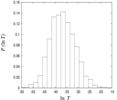
FIG. 5.: Normalized histogram of the logarithm of the conductance $T$ in the localized regime, for a network of linear size $L=60$ and a fixed distance $r=7$ between the contacts.

Fig. 5 shows a normalized histogram accumulated from $3000$ data points for the logarithm of the conductance $g=T$ (in atomic units), at fixed values of the distance $r=7$ and the system size $L=60$. The histogram clearly demonstrates the approximate log-normal character of the distribution. Such behavior is expected from the standard picture of localization. More precisely, the picture says that the inverse of localization length $\xi$ has a normal distribution (see [4] for a review), and the conductance is given by $g=g_{0}\exp(-2r/\xi)$ where the factor of $2$ is due to the convention of associating the localization length with the modulus of the wavefunction. The inverse of the average of $1/\xi$ is called the typical value $\xi_{\rm t}$ of the localization length: $\xi_{\rm t}^{-1}=\left\langle\xi^{-1}\right\rangle$. As a further check on this picture, we calculated $\left\langle\ln T\right\rangle$ as a function of $r$ and found linear behavior, as shown in Fig. 6. The average was performed as a combination of spatial average and disorder average accumulating 3000 data.

FIG. 6.: Plot of the average of $\ln T$ versus the distance $r$ between the contacts, for different system sizes $L$ and probabilities $p=(1+{\rm e}^{-E})^{-1}$.

A more interesting question concerns the relation between the two parameters (log-mean $\left\langle\ln T\right\rangle$ and log-variance $\left\langle(\delta\ln T)^{2}\right\rangle$) of the log-normal distribution. According to the one-parameter scaling hypothesis first formulated in [30], one expects the two parameters to be dependent on each other. Such a dependence was indeed observed in other LD transitions (see e.g. [31]), and it takes the form of a linear relation

$$\left\langle(\delta\ln T)^{2}\right\rangle=-A\left\langle\ln T\right\rangle+B\,,$$ (11)

where $A$ is a number of order unity (it equals $2$ in quasi-1D systems [32]), and $B$ is some offset due to the presence of the factor $g_{0}$. Our data confirm this picture. The value for $A$ we find is $A=1.00\pm 0.05$ (Fig. 7). Thus, the typical localization length is the only relevant parameter for the conductance distribution in the localized regime. This distribution is very broad and is well described by a log-normal form.

FIG. 7.: Linear relation between the mean and the variance of the conductance distribution in the localized regime.

IV Point-contact conductances at criticality

We now embark on an investigation of point-contact conductances of the critical network model at $p^{\ast}=1/2$, by employing a combination of analytical and numerical techniques. In subsection IV A, the network model is mapped on a supersymmetric vertex model (for technically related work see also [18]) and the $q^{\rm th}$ moment of the transmission coefficient $T$ is expressed as a two-point correlator (Eqs. (14, 15)). For this we follow the method of [17], which is based on the so-called color-flavor transformation and is included here for completeness. In subsection IV B we take advantage of the global symmetries of the vertex model and, based on the general principles of conformal field theory, propose a closed analytical expression for the $q^{\rm th}$ moment of the point-contact conductance at criticality (Eq. (20)). This expression is analytically continued to $q=0$, to extract predictions for the typical conductance and the log-variance, which are compared to numerical data in subsection IV C. In the limit of large separation between the contacts, which is difficult to reach numerically, a multifractal description of conductances becomes appropriate, as is discussed in subsection IV D. In subsection IV E we use conformal invariance to predict an exact expression for point-contact conductances in the quasi one-dimensional limit of the network model. Finally, in subsection IV F we reconstruct from the moments the entire distribution function of point-contact conductances.

A Mapping on a supersymmetric vertex model

We start by recalling the Landauer-Büttiker formula for the dimensionless conductance: $g=T\equiv|t_{c^{\prime}c}|^{2}$, where

$$t_{c^{\prime}c}=\langle c^{\prime}|(1-U_{P})^{-1}U|c\rangle\;.$$

For the following it is convenient to change our conventions slightly and interpret each of the severed contact links $c$ and $c^{\prime}$ as a pair of disjoint links (Fig. 4), defining basis states $|{i_{1}}\rangle$, $|{o_{1}}\rangle$ and $|{i_{2}}\rangle$, $|{o_{2}}\rangle$ respectively. We then impose the boundary conditions

$$U|o_{1}\rangle = 0=U|o_{2}\rangle\;,$$ (12)

$$U^{\dagger}|i_{1}\rangle = 0=U^{\dagger}|i_{2}\rangle\;.$$ (13)

The boundary conditions on the outgoing links have the same effect as the projectors $P_{c}$ and $P_{c^{\prime}}$, which enter in the definition $U_{P}=U(1-P_{c}-P_{c^{\prime}})$. With these boundary conditions in force, we can write the expression for the transmission amplitude as $t_{c^{\prime}c}=\langle o_{2}|(1-U)^{-1}U|i_{1}\rangle$. Assuming the two point contacts to be separated by more than one lattice unit, so that $\langle o_{2}|U|i_{1}\rangle=0$, we can write it in the even simpler form

$$t_{c^{\prime}c}=\langle o_{2}|(1-U)^{-1}|i_{1}\rangle\;.$$

Note that the escape of flux, here modeled by the boundary conditions on the outgoing links, causes a unitarity deficit and thus ensures positivity of the operator $1-U^{\dagger}U$.

The next step is to express $t_{c^{\prime}c}$ as a Gaussian superintegral. For this purpose we introduce a doublet $\Psi=(\Psi_{\rm B},\Psi_{\rm F})$ for every link. (The incoming and outgoing ones are included.) The quantities $\Psi_{\rm B}$ and $\Psi_{\rm F}$ are bosonic and fermionic (i.e. commuting and anticommuting) complex integration variables. Defining a Gaussian “statistical” average by

$$\left\langle\bullet\right\rangle=\int\bullet\ \exp-S_{+}$$

with

$$S_{+}=\sum_{\sigma={\rm B,F}}\sum_{l,l^{\prime}}\bar{\Psi}_{\sigma}(l^{\prime})(\delta_{l^{\prime}l}-U_{l^{\prime}l})\Psi_{\sigma}(l)\;,$$

we have

$$t_{c^{\prime}c}=\left\langle\Psi_{\rm B}(o_{2})\bar{\Psi}_{\rm B}(i_{1})\right\rangle\;.$$

As usual the integration measure for the field $\Psi$ is the flat one, normalized so that $\left\langle 1\right\rangle=1$. The Gaussian integral over $\Psi$ converges because the modulus of the operator $U$ with boundary condition (12) is less than unity.

Our interest here is not only in the average conductance but in all moments of the conductance. In fact, we ultimately will reconstruct the entire distribution function. To calculate the $q^{\rm th}$ moment we need an expression for the $q^{\rm th}$ power of $t_{c^{\prime}c}$. As is easily verified from Wick’s theorem, this is given by

$$t_{c^{\prime}c}^{q}={1\over q!}\left\langle\Psi_{\rm B}(o_{2})^{q}\bar{\Psi}_{\rm B}(i_{1})^{q}\right\rangle\;.$$

Note that in a many-channel situation (such as a network model with more than one channel per link or a conductance which is not point contact) where $t_{c^{\prime}c}$ consists of more than one amplitude, going from $q=1$ to arbitrary $q$ requires enlarging $\Psi$ to a superfield with more than one component. Here we are in the fortunate situation that a single component suffices to generate all the moments [33].

We call $\Psi$ a “retarded” field and denote it from now on by $\Psi_{+}$. The complex conjugate $\overline{t_{c^{\prime}c}}$ is expressed by a similar construction using an “advanced” field, $\Psi_{-}$. By combining the Gaussian integrals over retarded and advanced fields we get

$$T^{q}={1\over q!^{2}}\left\langle\Psi_{+{\rm B}}(o_{2})^{q}\bar{\Psi}_{+{\rm B}}(i_{1})^{q}\Psi_{-{\rm B}}(i_{1})^{q}\bar{\Psi}_{-{\rm B}}(o_{2})^{q}\right\rangle$$

for the $q^{\rm th}$ moment of the transmission probability. The Gaussian statistical average here is taken with respect to $\exp-S$ where $S=S_{+}+S_{-}$ and

$$S_{-}=\sum_{\sigma={\rm B,F}}\sum_{l,l^{\prime}}\bar{\Psi}_{-\sigma}(l)(\delta_{ll^{\prime}}-\bar{U}_{l^{\prime}l})\Psi_{-\sigma}(l^{\prime})\;.$$

Our next goal is to average over the disorder of the network model. For that we put

$$U_{l^{\prime}l}=U_{1}(l^{\prime},l)\ {\rm e}^{i\varphi(l)}$$

where $U_{1}$ is the deterministic part of $U$ describing the scattering at the nodes, and $\varphi(l)$ are random phases uniformly distributed on the interval $[0,2\pi]$. On extracting from $\exp-S$ the $\varphi$-dependent parts and temporarily omitting the integration over the superfield $\Psi$, we are faced with the integral

$${\cal F}=\int\prod_{l}{d\varphi(l)\over 2\pi}\exp\sum_{\sigma;l^{\prime},l}\Big{(}\bar{\Psi}_{+\sigma}(l^{\prime})U_{1}(l^{\prime},l){\rm e}^{i\varphi(l)}\Psi_{+\sigma}(l )$$

$$+\bar{\Psi}_{-\sigma}(l){\rm e}^{-i\varphi(l)}U_{1}^{\dagger}(l,l^{\prime})\Psi_{-\sigma}(l^{\prime}) \Big{)}\;.$$

It is seen that the random phases ${\rm e}^{\pm i\varphi}$ couple, roughly speaking, to the bilinears $\sum_{\sigma}\bar{\Psi}_{\pm\sigma}\Psi_{\pm\sigma}$. Plain integration over the variables $\varphi(l)$ now produces a product of Bessel functions, an expression which is not a good starting point for further analysis. Fortunately, there exists something better we can do. In the supersymmetric treatment [34] of disordered Hamiltonian systems, one makes a Hubbard-Stratonovitch transformation replacing the disorder average by an integral over a supermatrix-valued field $Q$. It turns out that a similar replacement, called the “color-flavor transformation” [35], can be made in the present context. The role of $Q$ is taken by two sets of complex fields $l\mapsto Z_{\sigma\sigma^{\prime}}(l)$ and $l\mapsto\tilde{Z}_{\sigma^{\prime}\sigma}(l)$, which assemble into supermatrices,

$$Z=\pmatrix{Z_{\rm BB}&Z_{\rm BF}\cr Z_{\rm FB}&Z_{\rm FF}\cr}\;,\quad\tilde{Z}=\pmatrix{\tilde{Z}_{\rm BB}&\tilde{Z}_{\rm BF}\cr\tilde{Z}_{\rm FB}&\tilde{Z}_{\rm FF}\cr}\;,$$

and couple to $\bar{\Psi}_{+\sigma}\Psi_{-\sigma^{\prime}}$ and $\bar{\Psi}_{-\sigma^{\prime}}\Psi_{+\sigma}$ respectively. The final outcome of the transformation will be another expression for ${\cal F}$, given at the end of the next paragraph, where instead of integrating over the random phases $\varphi(l)$ we integrate over the supermatrix fields $Z,\tilde{Z}$.

For completeness, let us now briefly summarize the mathematical structures surrounding the supermatrices $Z$ and $\tilde{Z}$. The details can be found in [36]. Elements $g=\pmatrix{A&B\cr C&D\cr}$ of the Lie supergroup $G_{{C}}\equiv{\rm GL}(2|2)$ are taken to act on $Z$, $\tilde{Z}$ by the transformations

$$Z\mapsto g\cdot Z = (AZ+B)(CZ+D)^{-1}\;,$$

$$\tilde{Z}\mapsto g\cdot\tilde{Z} = (C+D\tilde{Z})(A+B\tilde{Z})^{-1}\;.$$

Because this group action is transitive and $Z=\tilde{Z}=0$ is fixed by an $H_{{C}}\equiv{\rm GL}(1|1)\times{\rm GL}(1|1)$ subgroup with elements $h=\pmatrix{A&0\cr 0&D\cr}$, the complex supermatrices $Z$ and $\tilde{Z}$ parameterize the complex coset superspace $G_{{C}}/H_{{C}}$. Let $D(Z,\tilde{Z})$ be a $G_{{C}}$ invariant superintegration measure on this coset space and put $D\mu(Z,\tilde{Z})=D(Z,\tilde{Z})\,{\rm SDet}(1-\tilde{Z}Z)$. We take the integration domain for the bosonic variables to be the Riemannian submanifold $M_{\rm r}$ defined by the conditions

$$\tilde{Z}_{\rm FF}=-\bar{Z}_{\rm FF}\;,\quad\tilde{Z}_{\rm BB}=+\bar{Z}_{\rm BB}\;,\quad|Z_{\rm BB}|^{2}<1\;.$$

The normalization of $D(Z,\tilde{Z})$ is fixed by requiring that $\int D\mu(Z,\tilde{Z})=1$. Given these definitions, it was shown in [36] that the above expression for ${\cal F}$ is equivalent to

$${\cal F}=\int{\cal D}\mu(Z,\tilde{Z})\ \exp\sum_{l\sigma\sigma^{\prime}}\Big{(}\bar{\Psi}_{-\sigma^{\prime}}(l)\tilde{Z}_{\sigma^{\prime}\sigma}(l)\Psi_{+\sigma}(l)$$

$$+(\bar{\Psi}_{+\sigma}U_{1})(l)Z_{\sigma\sigma^{\prime}}(l)(U_{1}^{\dagger}\Psi_{-\sigma^{\prime}})(l)\Big{)}\;,$$

where ${\cal D}\mu(Z,\tilde{Z})=\prod_{l}D\mu(Z(l),\tilde{Z}(l))$. It is understood that the sum over $l$ excludes all links leaving the network. Indeed, by the boundary condition (12) the phase $\varphi(l)$ on an outgoing link $l=o_{1}$ or $l=o_{2}$ never appears in the formalism and there is no need to introduce any supermatrices $Z,\tilde{Z}$ there. Alternatively, we may extend the sum to run over all links and compensate by putting

$$Z(l)=\tilde{Z}(l)=0\quad\mbox{for all outgoing links}.$$

We mention in passing that the equivalence between the two expressions for ${\cal F}$ extends [17] to the more general case where the random phase factors ${\rm e}^{i\varphi(l)}\in{\rm U}(1)$ on links are replaced by random ${\rm U}(N)$ elements. The transformation from these ${\rm U}(N)$ “gauge” degrees of freedom to composite “gauge singlets” $Z(l),\tilde{Z}(l)$ is in striking analogy with strongly coupled ${\rm U}(N)$ lattice quantum chromodynamics, where integration over the gauge fields, which carry ${\rm U}(N)$ color, produces an effective description in terms of meson fields carrying flavor. Therefore, the passage from the first form of ${\cal Z}$ to the second one is referred to as the “color-flavor transformation” [35].

An attractive feature of the color-flavor transformation is that it preserves the Gaussian dependence of the integrand on the fields $\Psi,\bar{\Psi}$. If we switch to schematic notation and suppress the link and super indices, the Gaussian statistical weight is the exponential of the quadratic form

$$-(\bar{\Psi}_{+}\ \bar{\Psi}_{-})\pmatrix{1&-U_{1}^{\vphantom{\dagger}}ZU_{1}^{\dagger}\cr-\tilde{Z}&1\cr}\pmatrix{\Psi_{+}\cr\Psi_{-}\cr}\;.$$

In the absence of source terms or other perturbations, integration over $\Psi,\bar{\Psi}$ simply produces the inverse of a superdeterminant,

$${\rm SDet}^{-1}\pmatrix{1&-U_{1}^{\vphantom{dagger}}ZU_{1}^{\dagger}\cr-\tilde{Z}&1\cr}={\rm SDet}^{-1}(1-\tilde{Z}U_{1}^{\vphantom{\dagger}}ZU_{1}^{\dagger})\;.$$

When the source terms are taken into account, additional factors arise. Since we are calculating a point-contact conductance, these are localized at two points. By applying Wick’s theorem, we get from the combination $\Psi_{-{\rm B}}(i_{1})^{q}\bar{\Psi}_{+{\rm B}}(i_{1})^{q}/q!$ at the first contact an extra factor

$$\left(\tilde{Z}(1-U_{1}^{\vphantom{\dagger}}ZU_{1}^{\dagger}\tilde{Z})^{-1}\right)_{\rm BB}(i_{1},i_{1})^{q}=\tilde{Z}_{\rm BB}^{q}(i_{1})\;.$$

The simplification to the right-hand side of this equation occurs because $U_{1}^{\dagger}(\bullet,i_{1})=0$ according to the boundary conditions (13). Unfortunately, a similar simplification does not take place at the other contact. (There is a basic asymmetry between “in” and “out”, which stems from the fact that we must decide on some ordering of the factors ${\rm e}^{i\varphi}$ and $U_{1}$ in the evolution operator for one time step.) However, we can mend the situation with a little trick. We “prolong the exit” by inserting an additional node on the out-links as shown in Fig. 8.

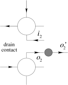
FIG. 8.: Prolongation of the exit by adding a dummy vertex at the drain contact, so as to simplify the field theoretic representation (see text) of the point-contact conductance.

This means that flux arriving at the link $o_{2}$ does not exit immediately, but first gets transferred to $o_{2}^{\prime}$ and then exits from there during the next time step. With this modification, the extra factor arising from the product $\Psi_{+{\rm B}}(o_{2}^{\prime})^{q}\bar{\Psi}_{-{\rm B}}(o_{2}^{\prime})^{q}/q!$ simplifies to

$$\left(U_{1}^{\vphantom{\dagger}}ZU_{1}^{\dagger}(1-\tilde{Z}U_{1}^{\vphantom{\dagger}}ZU_{1}^{\dagger})^{-1}\right)_{\rm BB}(o_{2}^{\prime},o_{2}^{\prime})^{q}=Z_{\rm BB}^{q}(o_{2})\;,$$

since $U_{1}(o_{2}^{\prime},o_{2}^{\vphantom{\prime}})=U_{1}^{\dagger}(o_{2}^{\vphantom{\prime}},o_{2}^{\prime})=1$ and $\tilde{Z}(o_{2}^{\prime})=0$.

In summary, we have expressed the $q^{\rm th}$ moment of the transmission coefficient $T$ as a two-point correlator,

$$\langle T^{q}\rangle=\left\langle Z_{\rm BB}^{q}(o_{2})\tilde{Z}_{\rm BB}^{q}(i_{1})\right\rangle\;,$$ (14)

of a supersymmetric lattice field theory,

$$\left\langle\bullet\right\rangle=\int{\cal D}\mu(Z,\tilde{Z})\;\bullet\;{\rm SDet}^{-1}(1-\tilde{Z}U_{1}^{\vphantom{\dagger}}ZU_{1}^{\dagger})\;.$$ (15)

The superdeterminant runs over superspace and the Hilbert space of the network model.

As it stands, the formula for $\langle T^{q}\rangle$ does not display clearly the internal symmetries of the theory. To make these more explicit, recall the definition of the (single $Z$) integration measure,

$$D\mu(Z,\tilde{Z})=D(Z,\tilde{Z})\ {\rm SDet}(1-\tilde{Z}Z)\;.$$

We now factor the superdeterminant as two square roots,

$${\rm SDet}(1-\tilde{Z}Z)={\rm SDet}^{1/2}(1-\tilde{Z}Z)\times{\rm SDet}^{1/2}(1-\tilde{Z}Z)\;,$$

and associate each of these with one of the two nodes a link begins or ends on. This procedure works perfectly for the internal links: every square root factor is assigned to exactly one node. For the external (or contact) links the situation is different. These are connected to just a single node of the network, and therefore only one of the two square roots is used up. It is natural to assign the remaining factor to the operator whose correlation function we are evaluating. In this way, the expression for $\langle T^{q}\rangle$ reorganizes to

$$\langle T^{q}\rangle=\left\langle v_{q}(o_{2})v_{0}^{\ast}(i_{2})\times v_{0}(o_{1})v_{-q}^{\ast}(i_{1})\right\rangle$$ (16)

where

$$v_{q} = Z_{\rm BB}^{q}\ {\rm SDet}^{1/2}(1-\tilde{Z}Z)\;,$$

$$v_{-q}^{\ast} = \tilde{Z}_{\rm BB}^{q}\ {\rm SDet}^{1/2}(1-\tilde{Z}Z)\;,$$

and

$$\left\langle\bullet\right\rangle = \int{\cal D}(Z,\tilde{Z})\ \bullet\ \exp-{\cal S}\;,$$

$${\cal D}(Z,\tilde{Z}) = \prod_{l}D(Z(l),\tilde{Z}(l))\;.$$

The statistical weight $\exp-{\cal S}$ is given by the superdeterminant ${\rm SDet}^{-1}(1-\tilde{Z}U_{1}^{\vphantom{\dagger}}ZU_{1}^{\dagger})$ multiplied by one (two) factors of ${\rm SDet}(1-\tilde{Z}(l)Z(l))$ for every external (internal) link. As was shown in [17], $\exp-{\cal S}$ has the structure of a vertex model weight, i.e. it separates into a product of factors, one for each node. Hence the lattice field theory with statistical weight $\exp-{\cal S}$ is called a vertex model. The factor for a given node, the so-called ${\cal R}$ matrix, is invariant under the global action of ${\rm GL}(2|2)$ or, more precisely speaking, can be regarded [17] as the matrix element of a ${\rm GL}(2|2)$ invariant operator between coherent states parametrized by the field variables $Z,\tilde{Z}$ on the links which emanate from that node.

B Symmetries and conformal hypothesis

The special significance of the functions $v_{q}^{\vphantom{\ast}}$ and $v_{-q}^{\ast}$ is that they lie [15] in irreducible representation spaces, denoted by $V$ and $V^{\ast}$, of the symmetry group ${\rm GL}(2|2)$. The action of ${\rm GL}(2|2)$ on these spaces can be shown to be unitary for a ${\rm SU}(1,1)\times{\rm SU}(2)$ subgroup, and $V$ and $V^{\ast}$ belong to the discrete series of ${\rm SU}(1,1)$. The representation space $V$ ($V^{\ast}$) is of lowest weight (resp. highest weight) type.

To make further progress, it is imperative that we exploit the global ${\rm GL}(2|2)$ symmetry of $\exp-{\cal S}$. The links $i_{1}$ and $o_{1}$ lie close in space, and so do $i_{2}$ and $o_{2}$, whereas these two sets are in general far apart from each other. Therefore, our next step is to fuse $v_{q}(o_{2})\in V$ with $v_{0}^{\ast}(i_{2})\in V^{\ast}$ and to make a decomposition into irreducible representation spaces of ${\rm GL}(2|2)$. The operators at the other contact, $v_{0}(o_{1})$ and $v_{-q}^{\ast}(i_{1})$, are processed in the same way. Thus we need to know how to reduce the tensor product $V\otimes V^{\ast}$. According to Sec. 5.2 of [15], this reduction involves a single continuous series of ${\rm GL}(2|2)$, which is closely related to the principal continuous series of unitary representations of ${\rm SU}(1,1)$. This series is labeled by a real parameter $\lambda\in[0,\infty)$. Denoting the basis state with weight $m$ by $\varphi_{\lambda m}$, we have

$$v_{q}^{\vphantom{\ast}}v_{0}^{\ast} = \int\left\langle Vq,V^{\ast}0|\lambda q\right\rangle\varphi_{\lambda q}\ \mu(\lambda)d\lambda\;,$$ (17)

$$v_{0}^{\vphantom{\ast}}v_{-q}^{\ast} = \int\left\langle V0,V^{\ast}{\rm-}q|\lambda{\rm-}q\right\rangle\varphi_{\lambda{\rm-}q}\ \mu(\lambda)d\lambda\;,$$ (18)

where $\left\langle Vm,V^{\ast}m^{\prime}|\lambda m+m^{\prime}\right\rangle$ is a Clebsch-Gordan coefficient, and $\mu(\lambda)d\lambda$ is the Plancherel measure for the continuous series labeled by $\lambda$. Explicit expressions for these will be given below. We adopt the convention $\overline{\varphi_{\lambda q}}=\varphi_{\lambda{\rm-}q}$. Then an immediate statement is that the Clebsch-Gordan coefficient behaves under complex conjugation as

$$\overline{\left\langle Vq,V^{\ast}0|\lambda q\right\rangle}=\left\langle V0,V^{\ast}{\rm-}q|\lambda{\rm-}q\right\rangle\;,$$

as follows from $\overline{v_{q}^{\vphantom{\ast}}v_{0}^{\ast}}=v_{0}^{\vphantom{\ast}}v_{-q}^{\ast}$.

All steps so far have been exact and rigorously justified. Now we have to make an assumption which is crucial, namely that the vertex model at $p^{\ast}=1/2$ flows under renormalization to a conformal fixed point theory. Sadly, although a substantial effort has been expended on identifying that fixed point, we still do not understand its precise nature. Nevertheless, as we shall see, we can draw a number of strong conclusions just from the assumption of its existence.

By the principles of conformal field theory, the two-point function of $\varphi_{\lambda}$ decays algebraically,

$$\left\langle\varphi_{\lambda q}({\bf r})\varphi_{\lambda^{\prime}{\rm-}q}({\bf r}^{\prime})\right\rangle={\delta(\lambda-\lambda^{\prime})\over\mu(\lambda)}|{\bf r}-{\bf r}^{\prime}|^{-2\Delta_{\lambda}}+\ldots$$ (19)

where $\Delta_{\lambda}$ is the scaling dimension of the most relevant conformal field contained in the expansion of $\varphi_{\lambda q}$. (By ${\rm GL}(2|2)$ invariance, this dimension is independent of the weight $q$.) Although $\Delta_{\lambda}$ cannot be predicted without knowing the stress-energy tensor of the conformal field theory, we will make an informed guess later on. What we can say right away is that $\Delta_{\lambda}$ must be an even function of $\lambda$. (This is due to the invariance of $\Delta_{\lambda}$ under a Weyl group action on the roots of the Lie superalgebra of ${\rm GL}(2|2)$, which takes $\lambda$ into $-\lambda$.) The appearance of the weight function $\mu(\lambda)$ in the denominator, and of the Dirac $\delta$-function (instead of the usual Kronecker $\delta$-symbol), are forced by the fact that we are dealing with a continuous series.

On inserting the decompositions (17) and (18) into the formula (16) for $\langle T^{q}\rangle$, and using the expression (19) for the two-point correlator, we obtain

$$\langle T^{q}\rangle=\int\big{|}\left\langle Vq,V^{\ast}0|\lambda q\right\rangle\big{|}^{2}r^{-2\Delta_{\lambda}}\mu(\lambda)d\lambda\;,$$ (20)

where $r$ is the distance between the two point contacts, measured in the units that are prescribed by the choice of normalization made in (19).

The computation of the Clebsch-Gordan coefficient and the Plancherel measure entering in the expression for $\langle T^{q}\rangle$ is nontrivial. Major complications arise from the fact that the modules $V$ and $V^{\ast}$ are infinite-dimensional, and that the representation spaces appearing in the decomposition of the tensor product $V\otimes V^{\ast}$ have neither a highest nor a lowest weight vector. Consequently, the computation cannot be done solely by algebraic means and a certain amount of analysis must be invested. We have relegated this lengthy calculation to the appendix, where it is shown that

$$\mu(\lambda)d\lambda = {\lambda\over 2}\tanh\left({\pi\lambda\over 2}\right)d\lambda\;,$$ (21)

$$\big{|}\left\langle Vq,V^{\ast}0|\lambda q\right\rangle\big{|}^{2} = {\Gamma(q-{1\over 2}-{i\lambda\over 2})\Gamma(q-{1\over 2}+{i\lambda\over 2})\over\Gamma(q)^{2}}\;.$$ (22)

As it stands, the result for $\langle T^{q}\rangle$ has been derived for all positive integers $q$. However, since the Clebsch-Gordan coefficient is a meromorphic function of $q$, it is clear that we can analytically continue the result to all $q$. (This analytic continuation is unique, as follows from the bound $|\langle T^{q}\rangle|\leq 1$ for ${\rm Re}(q)>0$ and Carlson’s theorem stated in paragraph 5.81 of [37].) Notice, now, that all of the $q$-dependence of $\langle T^{q}\rangle$ resides in the Clebsch-Gordan coefficient, while the dependence on $r$ is encoded in the factor $r^{-2\Delta_{\lambda}}$. It would therefore seem that all moments of $T$ decay asymptotically with the same power, $\langle T^{q}\rangle\sim r^{-2\Delta_{0}}$, the exponent being given by $\Delta_{0}={\rm Min}_{\lambda\in{{R}}^{+}}\Delta_{\lambda}$. While this is correct for $q\geq 1/2$, it fails to be true for $q<1/2$. The reason is that, when $q$ is lowered past the value 1/2 from above, the two poles at $\lambda=\pm i(2q-1)$ of the gamma functions $\Gamma(q-{1\over 2}\pm{i\lambda\over 2})$ cross the integration axis at $\lambda=0$. Therefore, to do the analytic continuation to $q<1/2$ correctly, we must pick up the contribution from these poles. It is straightforward to calculate the residues at the poles, which results in

$$\langle T^{q}\rangle = \Gamma(q)^{-2}\int_{0}^{\infty}\big{|}{\textstyle\Gamma(q-{1\over 2}-{i\lambda\over 2})}\big{|}^{2}r^{-2\Delta_{\lambda}}\mu(\lambda)d\lambda$$ (23)

$$+ 2\pi\cot(q\pi){\Gamma(2q)\over\Gamma(q)^{2}}\ r^{-2\Delta_{i(2q-1)}}\quad(|q|<1/2)\;.$$ (24)

Here we have used $\Delta_{\lambda}=\Delta_{-\lambda}$ to combine terms.

By letting $q$ go to zero in (24) and using the fact that normalization of the distribution function for $T$ implies $\langle T^{q}\rangle\big{|}_{q=0}=1$, we can deduce a constraint on $\Delta_{\lambda}$. Indeed, from (22) the square of the Clebsch-Gordan coefficient vanishes uniformly in $\lambda$ as $q\to 0$, and since $\lim_{q\to 0}2\pi\cot(q\pi)\Gamma(2q)/\Gamma(q)^{2}=1$, we have $\langle T^{0}\rangle=r^{-2\Delta_{-i}}$. Hence we conclude

$$\Delta_{-i}=\Delta_{+i}=0\;.$$

Thus, normalization constrains $\Delta_{\lambda}$ to be of the form

$$\Delta_{\lambda}=(\lambda^{2}+1)F(\lambda^{2})\;.$$

It will be convenient to set $F(\lambda^{2})=f(\lambda^{2}+1)$.

C Typical conductance and log-variance

Our next goal is to obtain information about the unknown function $f$. Because we have no analytical control on the fixed point theory, we are forced to resort to numerical means. To prepare the numerical calculation, we first show that $f(0)$ is determined in a very simple way by how the typical conductance $\exp\langle\ln T\rangle$ varies with $r$. To that end we differentiate both sides of (24) with respect to $q$ at $q=0$ and use the identity

$${d\over dq}\langle T^{q}\rangle\big{|}_{q=0}=\langle\ln T\rangle\;.$$

The integral on the right-hand side of (24) tends to a finite value while $\Gamma(q)^{-2}$ behaves as $q^{2}$ in the limit $q\to 0$. Also, the Taylor expansion of $2\pi\cot(q\pi)\Gamma(2q)/\Gamma(q)^{2}=1+{\cal O}(q^{2})$ contains no term linear in $q$, as is easily verified from standard properties of the gamma function. Hence

$$\langle\ln T\rangle={d\over dq}r^{-2\Delta_{i(2q-1)}}\big{|}_{q=0}=-8f(0)\ln r\;,$$

or, after exponentiation,

$$\exp\langle\ln T\rangle=r^{-X_{\rm t}}\;,\quad X_{\rm t}=8f(0)\;.$$ (25)

Thus, $\exp\langle\ln T\rangle$ decays as a pure power. Note that this feature is unique to the typical conductance. For a general value of $q$, formula (24) shows that the behavior of $\langle T^{q}\rangle$ as a function of $r$ is governed by a whole continuum of exponents.

We have calculated conductances at criticality ($p=p^{\ast}=0.5$) for systems of size $L=40$, $60$, and $100$, and for distances $r$ varying from $r=1$ to $r=L/2$. For every distance, $2200$ realizations for $L=40$, $1200$ realizations for $L=60$, and between $200$ and $300$ realizations for $L=100$, were generated.

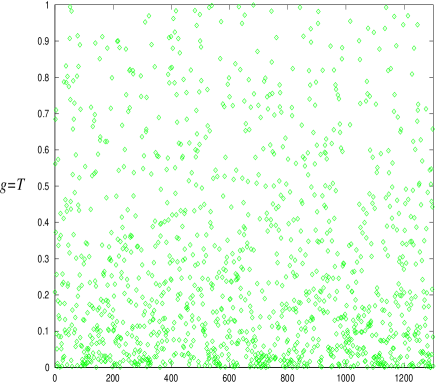
FIG. 9.: Fluctuating values of the conductance $g$ (or the transmission probability $T$) at the critical point of the network model. 1300 realizations at a fixed distance $r=10$ are displayed.

Fig. 9 shows $1300$ realizations of the conductance for $L=60$ and $r=10$. The distribution of conductances is seen to be very broad. In Fig. 10 the mean logarithm of the conductance, $\left\langle\ln T\right\rangle$, is displayed as a function of $\ln r$ for three different system sizes $L=40,60,100$.

FIG. 10.: Scaling plot of the typical conductance for three different system sizes. The horizontal and vertical axes are logarithmic.

The typical value indeed scales as a power with $r$,

$$\exp\langle\ln T\rangle = (r/r_{0})^{-X_{\rm t}}\,,$$ (26)

$$X_{\rm t} = 0.640\pm 0.009\,,\quad r_{0}\approx 0.42\,,$$ (27)

and has no significant dependence on the system size. The result for $X_{\rm t}$ is based on data for $L=100$ and distances $r\leq 40$, on data for $L=60$ and distances $r\leq 25$, and on data for $L=40$ and distances $r\leq 20$. The error results from a linear fit taking the statistical errors of the data into account. Taking the same raw data but neglecting their errors, yields $X_{\rm t}=0.613\pm 0.012$. Note that the hypothesis (19) was formulated in “conformal units” ($r_{0}=1$) whereas the numerical data are represented in length units given by the lattice constant of the network. Therefore, $r_{0}$ is written explicitly in Eq. (27) whereas it is treated as unity in Eq. (25).

Higher moments of $\ln T$ can be obtained by using $\langle T^{q}\rangle$ as a generating function:

$$\langle T^{q}\rangle=1+q\langle\ln T\rangle+(q^{2}/2)\langle(\ln T)^{2}\rangle+\ldots$$

A straightforward calculation starting from (24) yields for the log-variance (in conformal units)

$$\langle(\ln T)^{2}\rangle - \langle\ln T\rangle^{2}=16\big{(}f(0)-4f^{\prime}(0)\big{)}\ln r$$ (28)

$$- \int_{0}^{\infty}(1-r^{-2\Delta_{\lambda}}){8\pi\ \mu(\lambda)d\lambda\over(\lambda^{2}+1)\cosh(\pi\lambda/2)}\;.$$ (29)

The integral on the right-hand side decays algebraically to a constant whereas the first term grows logarithmically. Eq. (29) says that the sum, $\Sigma$, of the log-variance and the integral is linear in $\ln r$. To obtain the prefactor of $\ln r$, we numerically calculated the integral for each value of $r$, took the log-variance from our data for systems of size $L=60$, and plotted the function $\Sigma(r)$ versus $X_{\rm t}\ln(r/r_{0})$, see Fig. 11. It turned out that the integral was nonnegligible for the range of $r$ values that were numerically accessible. The slope of the straight line in Fig. 11 is $2.08\pm 0.11$, i.e. the log-variance is about twice the log-average for large $r$ (as is the case for in quasi-1D systems [32]). Given $8f(0)=X_{\rm t}$, our numerical result implies that $f^{\prime}(0)$ is very close to zero:

$$-4f^{\prime}(0)/X_{\rm t}=0.005\pm 0.008\;,$$

which leads us to conjecture $f^{\prime}=0$ or, equivalently, a dependence of $\Delta_{\lambda}$ which is exactly quadratic:

$$\Delta_{\lambda}=f(0)(\lambda^{2}+1)={X_{\rm t}\over 8}(\lambda^{2}+1)\;.$$ (30)

Aside from being the simplest possible expression for $\Delta_{\lambda}$, this guess is in line with field theoretic expectations: in conformal field theories with a stress-energy tensor that is quadratic in the currents, the scaling dimensions are proportional to the quadratic Casimir invariant. The polynomial $\lambda^{2}+1$ is, in fact, the quadratic Casimir of ${\rm GL}(2|2)$, evaluated on the continuous series of representations $\lambda$. In the language of multifractality (Sec. IV D), the conjecture (30) means that the parabolic approximation to the $F(a)$ spectrum is exact. In the remainder of the present paper we shall assume the quadratic form (30).

FIG. 11.: The log-variance of the conductance augmented by the integral on the right-hand side of (29) is denoted by $\Sigma(r)$ and plotted versus $X_{\rm t}\ln(r/r_{0})$.

D Multifractal spectrum

We have seen that the dependence of $\langle T^{q}\rangle$ on the distance between the two point contacts is governed in general by a continuous set of exponents $2\Delta_{\lambda}$. This dependence simplifies, of course, in the asymptotic domain $r\to\infty$. For $q\geq 1/2$ the asymptotic behavior is controlled by the smallest exponent, $2\Delta_{0}=X_{\rm t}/4\simeq 0.16$. In the range $-1/2\leq q\leq+1/2$, the dominant contribution comes from the second term on the right-hand side of Eq. (24), with the exponent being $2\Delta_{i(2q-1)}=X_{\rm t}q(1-q)\leq X_{\rm t}/4$. For $q\leq-1/2$ there appear additional contributions due to the poles of $\Gamma(q-{1\over 2}\pm{i\lambda\over 2})$ at $\lambda=\pm i(2q+1)$, $\pm i(2q+3)$, etc. However, since $\Delta_{i(2q-1)}<\Delta_{i(2q+1)}<\Delta_{i(2q+3)}<\ldots$ for $q<-1/2$, these are negligible in the limit $r\to\infty$. Thus we have

$$\langle T^{q}\rangle\ {\buildrel r\to\infty\over{\sim}}\ r^{-X(q)}\;,$$ (31)

$$X(q)=\left\{\matrix{X_{\rm t}/4&{\rm for}\ q\geq 1/2\;,\cr X_{\rm t}q(1-q)&{\rm else}\;.\cr}\right.$$ (32)

Note that the spectrum of exponents $X(q)$ is a nondecreasing function of $q$. The spectrum shown in Fig. 12 is nonlinear, as is characteristic of a multifractal.

FIG. 12.: The multifractal spectrum $X(q)$ governing the asymptotic power law scaling of the moments $\langle T^{q}\rangle$.

That $X(q)$ becomes constant for $q\geq 1/2$ can be traced to the boundedness of the variable $\ln T\leq 0$: for $q\geq 1/2$ the asymptotics of the moment $\langle T^{q}\rangle$ is governed by the value of the distribution function at the upper bound, ${\rm prob}(T=1;r)\sim r^{-X_{\rm t}/4}$, which is independent of $q$, as is $T^{q}\big{|}_{T=1}$. In a thermodynamic interpretation of multifractal spectra, the nonanalyticity at $q=1/2$ is called a “phase transition” in $X(q)$ [38]. The failure of $X(q)$ to become linear for $q\to-\infty$ results from the absence of a lower bound on $\ln T$.

The multifractal nature of the $X(q)$ spectrum can alternatively be described by a spectrum of $f(\alpha)$ type. If we make a multifractal ansatz for the probability density of $T$,

$${\rm prob}(T=r^{-a})\ {\rm d}T\sim r^{-F(a)}{\rm d}a\;,$$

the moments of $T$ for large $r$ scale as

$$\langle T^{q}\rangle\sim\int r^{-qa-F(a)}da\sim r^{-X(q)}\;,$$

where $X(q)$ and $F(a)$ are Legendre transforms of each other, i.e. $q+F^{\prime}(a(q))=0$, $X(q)=qa(q)+F(a(q))$, and conversely, $a-X^{\prime}(q(a))=0$, $F(a)=-aq(a)+X(q(a))$. Using these relations we find

$$F(a)={(a-X_{\rm t})^{2}\over 4X_{\rm t}}\quad(a>0)\;.$$ (33)

The $F(a)$ spectrum shown in Fig. 13 is defined only for positive values of $a$ because $a=X^{\prime}(q)\geq 0$.

FIG. 13.: The multifractal spectrum $F(a)$ describing the scaling of the distribution ${\rm prob}(T=r^{-a}){\rm d}T$.

An obvious question arises: is it possible to relate the multifractal exponents $X(q)$ to the $\tau(q)$ spectrum of the critical eigenstates, or the scaling exponents of the LDoS? Our first observation is that there exists an obvious difference between the two cases: while the spatial correlations of the LDoS continue to scale in a nontrivial manner with system size $L$ when $L$ is increased, the distribution of point-contact conductances (at fixed $r$) becomes independent of $L$ [15]. Another way of saying this is that the critical conductance between interior point contacts has a trivial infinite volume limit, whereas the LDoS does not.

To explain this distinction in physical terms, recall the iterative procedure by which the stationary limit $\psi_{\infty}$ was approached. An essential ingredient in that process was the draining action of the broken links at the two contacts. By the loss of probability through these outgoing channels, the system relaxes and settles down to a stationary long-time limit. The key to understanding the size dependence of the conductance is to visualize the distribution of $|\psi_{\infty}|^{2}$ in space. In the regime of localized states this distribution is concentrated in a circular area of radius $\sim\xi$ centered around its source (i.e. the contact where the current is fed in). Outside this area the intensity $|\psi_{\infty}|^{2}$ falls off exponentially with distance. On approaching the critical point, $\xi$ diverges and the exponential decay turns into a power law. Thus the intensity becomes more spread out. However, in spite of this spreading out, the intensity remains (algebraically) localized near the source. The finite size of the network affects only the tails of the distribution $|\psi_{\infty}|^{2}$ and, as a result, the conductance converges to a well-defined limit as the system size goes to infinity.

When the LDoS is discussed in the same language, a different picture emerges. Consider, for simplicity, the $q^{\rm th}$ power of the density-density correlator

$$\left|\langle c^{\prime}|(1-{\rm e}^{-\delta}U)^{-1}|c\rangle\right|^{2q}$$

which, though not expressible as a correlation function of the LDoS, is related closely enough to allow a meaningful comparison. There again exists a dynamical interpretation. To compute the density-density correlator we feed in current through link $c$ and, after relaxation to the steady state, measure the square of the amplitude at link $c^{\prime}$. What is different from the conductance measurement is that there are no drains at $c$ and $c^{\prime}$ (the network is now isolated). Instead, particles are absorbed at a constant rate $2\delta$ at any location in the network. As the system size is increased, the time spent in the network grows as the Heisenberg time $\delta^{-1}\sim L^{d}$. (Previously, the dwell time in the 2D network was limited by the “strength” of the contacts and remained finite in the limit $L\to\infty$.) Thus, there is a build up of particles in the network. When all states are localized, this causes the $q$-dependent correlator to diverge as $\delta^{-q}\sim L^{qd}$. At the critical point, the divergence from build up is counteracted by the reduction in the amplitude at link $j$ due to incipient delocalization of the wavefunctions. For a general value of $q$ the two competing effects do not cancel, so that a nontrivial scaling with $L$ is expected to remain, in agreement with what we found in Sec. II.

Having said all this, we return to the original question: is it possible, after all, to relate the multifractal exponents $X(q)$ to the $\tau(q)$ spectrum? We wish to offer the following argument. Imagine placing tunnel barriers at the two contacts $c,c^{\prime}$. For zero tunneling probability, the network is closed and we can measure the density-density correlations. Now assume that the $q$-dependent density-density correlator has the same set of scaling exponents as the LDoS correlator. Then, in the limit $\omega=0$ (or $L_{\omega}=\infty$) we have

$$\left\langle\Big{|}\langle c^{\prime}|(1-{\rm e}^{-\delta}U)^{-1}|c\rangle\Big{|}^{2q}\right\rangle\sim r^{-z(q)}L^{z(q)-\tilde{z}(q)}\;.$$

As the tunneling rate is increased, a new time scale appears: the time a particle injected at link $c$ spends in the network (with the absorption rate $\delta$ set to zero) before exiting through link $c^{\prime}$. The critical dynamics translates this dwell time into some characteristic length, $L_{\tau}$. Although $L_{\tau}$ is an irrelevant length for an almost closed system with high tunnel barriers, it takes the regularizing role of the system size in the regime of open systems with $L_{\tau}<L$. In the limit of vanishing tunnel barriers, the density-density correlator turns into the point-contact conductance. At the same time, the length $L_{\tau}$ must become proportional to the distance between the point contacts, for the simple reason that no other length scale remains available. This argument would say $\langle T^{q}\rangle\sim r^{-\tilde{z}(q)}$, and suggests $\tilde{z}(q)$ as a candidate for $X(q)$. We should be cautioned by the fact that the density-density correlator, unlike the conductance, does not respect any upper bound. This difference influences the tails of the distribution and changes the high moments, at least. In fact, we have shown $X(q)$ to be constant for $q\geq 1/2$, whereas $\tilde{z}(q)$ continues to increase. However, the tails of the distribution should not affect the typical values, and therefore one might expect $X_{\rm t}=X^{\prime}(0)=\tilde{z}^{\prime}(0)=2(\alpha_{0}-2)$. Recall that we found $X_{\rm t}=0.640\pm 0.009$. Other groups quote values $2(\alpha_{0}-2)=0.56\pm 0.04$ [16], $0.54\pm 0.02$ (e.g. [3]), and $0.58\pm 0.04$ [39]. These values are not all mutually consistent. We leave it as an open problem whether there is a flaw in the argument linking $X(q)$ with $\tilde{z}(q)$ or there is a real discrepancy.

E Quasi-1D limit

We now endow the network model with a cylinder geometry. This means that we consider an infinitely long strip of width $W$, with coordinates $x\in{{R}}$ and $y\in[0,W]$, and impose periodic boundary conditions in the transverse direction. As before, our interest is in the conductance between two point contacts, which are placed at positions $(x,y)$ and $(x^{\prime},y^{\prime})$. The conductance in such a cylindrical setting can be related to the point-contact conductance in the infinite 2D plane with complex coordinate $z$ by a conformal transformation

$$z=\exp\ {2\pi\over W}(x+iy)\;.$$

The conformal field theory rule for translating two-point functions from the plane to the cylinder reads [40]

$$\langle\varphi_{\lambda}(z)\varphi_{\lambda}(z^{\prime})\rangle=|z-z^{\prime}|^{-2\Delta_{\lambda}}$$

$$\to\left|{W\over\pi}\sinh\left({\pi\over W}(x-x^{\prime}+iy-iy^{\prime})\right)\right|^{-2\Delta_{\lambda}}\;.$$

From this rule we have the relation

$$\langle T^{q}\rangle\big{|}_{(x,y);(x^{\prime},y^{\prime})}^{\rm cylinder}=\langle T^{q}\rangle\big{|}_{r=|{W\over\pi}\sinh({\pi\over W}(x-x^{\prime}+iy-iy^{\prime}))|}^{\rm 2D}\;.$$

In particular, for the typical cylindrical conductance we obtain

$$\exp\langle\ln T\rangle=\left|{W\over\pi}\sinh\left({\pi\over W}(x-x^{\prime}+iy-iy^{\prime})\right)\right|^{-X_{\rm t}}\;.$$

(Recall that we are using length units so that $\langle\ln T\rangle_{2{\rm D}}=0$ for $r=1$.) In the quasi-1D limit $L\equiv|x-x^{\prime}|\gg W$, this result simplifies to

$$\exp\langle\ln T\rangle\big{|}_{L\gg W}=(W/2\pi)^{X_{\rm t}}\exp-\pi X_{\rm t}L/W\;.$$

Note that from (27) the numerical value of $\pi X_{\rm t}$ is

$$\pi X_{\rm t}=2.01\pm 0.03\;.$$ (34)

What is this result, a value of $\pi X_{\rm t}$ close to 2, trying to tell us? Let us offer some speculation based on the assumption that the relation $\pi X_{\rm t}=2$ holds exactly. In [17] it was shown that, if a naive continuum limit is assumed (i.e. possible renormalization effects due to short wave length modes are ignored), the supersymmetric vertex model (15) for the critical network is equivalent to Pruisken’s nonlinear $\sigma$ model [41] at couplings $\sigma_{xx}=\sigma_{xy}=1/2$. The action functional of the latter model is

$${\cal S}=\int dxdy\ \Big{(}\sigma_{xx}({\cal L}_{xx}+{\cal L}_{yy})+\sigma_{xy}({\cal L}_{xy}-{\cal L}_{yx})\Big{)}\;,$$

where

$${\cal L}_{\mu\nu}={\rm STr}(1-Z\tilde{Z})^{-1}\partial_{\mu}Z(1-\tilde{Z}Z)^{-1}\partial_{\nu}\tilde{Z}\;.$$

For the sake of the argument, let us now assume Pruisken’s model at $\sigma_{xx}=\sigma_{xy}=1/2$ to be a fixed point of the renormalization group. Then, by raising the short distance cutoff from $a=1$ to $a=W$ we can reduce Pruisken’s action ${\cal S}$ to a 1D effective action

$${\cal S}_{1{\rm D}}={W\over 2}\int dx\ {\rm STr}(1-Z\tilde{Z})^{-1}\partial_{x}Z(1-\tilde{Z}Z)^{-1}\partial_{x}\tilde{Z}\;.$$

Alternatively, we could argue that in the quasi-1D limit the dependence of the field $Z$ on $y$ can be neglected and, since $\sigma_{xx}$ does not renormalize (by the fixed point hypothesis), the process of scaling out $y$ simply produces a factor $\int dy=W$.

The one-dimensional theory with action functional ${\cal S}_{1{\rm D}}$ has been much studied, and its mean conductance is known [42, 43, 44] to decay with length $L$ of the conductor, which plays the role of distance between the contacts, as

$$\langle T\rangle\big{|}_{L}^{\rm 1D}\sim\exp-L/2W\;.$$

Moreover, from [45] we know that the localization lengths for the mean and typical conductances of the one-dimensional nonlinear $\sigma$ model differ by a factor of 4, so that

$$\exp\langle\ln T\rangle\big{|}_{L}^{\rm 1D}\sim\exp-2L/W\;,$$

which agrees, within the numerical errors, with what we found in (34). To turn the argument around, by assuming Pruisken’s nonlinear $\sigma$ model at $\sigma_{xx}=\sigma_{xy}=1/2$ to be a fixed point, we would have predicted $X_{\rm t}$ to be

$$X_{\rm t}=(\pi\sigma_{xx})^{-1}\big{|}_{\sigma_{xx}=1/2}\approx 0.637\;.$$

The above argument is not convincing, as it relies on the questionable assumption that the nonlinear $\sigma$ model is a fixed point theory. Conventional wisdom has it that critical two-dimensional nonlinear $\sigma$ models are unstable with respect to quantum fluctuations and flow under renormalization to theories of the Wess-Zumino-Witten type. However, we can reformulate the argument and avoid any reference to Pruisken’s theory. Let us assume that it is the network model itself (or, rather, a suitable continuum limit thereof) which is a fixed point of the renormalization group. Note that such an assumption is consistent with the fact that network model observables start scaling very rapidly when the observation scale is increased. (For example, in Fig. 10 there are no visible deviations from linearity as $r$ approaches the short distance cutoff $a$.) As before, we imagine raising the cutoff by using a sequence of RG transformations. By the fixed point hypothesis, we arrive for $a=W$ at the 1D network model (or, rather, some continuum version closely related to it), with the distance between contacts rescaled to $L/W$. Next we pass to the 1D supersymmetric vertex model, and from there to the continuum action ${\cal S}_{1{\rm D}}$. In contrast to earlier, the last step is benign, as the 1D nonlinear $\sigma$ model is superrenormalizable (i.e. ultraviolet finite) and the RG trajectory can no longer depart from it. By this token, we again arrive at $X_{\rm t}=2/\pi$, this time without having passed through Pruisken’s model. Thus, the proposed value for $X_{\rm t}$ follows as a consequence of assuming the network model (or a suitable continuum limit thereof) to be a RG fixed point.

Note that if the above fixed point assumption is correct and $X_{\rm t}=2/\pi$ holds exactly, then we are led to the striking conclusion that Wess-Zumino-Witten models are ruled out as candidates for the fixed point theory. Indeed, the scaling dimensions for such models are given [46] by ${\cal C}_{\lambda}/(k+h_{\ast})$, where ${\cal C}_{\lambda}$ is the quadratic Casimir, and $k$ and $h_{\ast}$ are integers. Such an expression for the scaling dimensions cannot produce the irrational number $2/\pi$.

F Reconstruction of the distribution

We now return to the two-dimensional network and reconstruct the entire distribution function for the point-contact conductance from the moments $\langle T^{q}\rangle$. By making a simple variable substitution (namely $x=2\rho+1$) in Eq. (A5) of the appendix, the product of gamma functions in the formula for $\langle T^{q}\rangle$ can be represented as an integral over Legendre functions:

$${|\Gamma(q-{1\over 2}-{i\lambda\over 2})|^{2}\over\Gamma(q)^{2}}=\int_{0}^{\infty}(1+\rho)^{-q}{\cal P}_{(i\lambda-1)/2}(2\rho+1)d\rho\;.$$

Next we define a probability density ${\rm prob}(\rho;r){\rm d}\rho$ for the variable $\rho$ by

$${\rm prob}(\rho;r)=\int_{0}^{\infty}r^{-X_{\rm t}(\lambda^{2}+1)/4}{\cal P}_{(i\lambda-1)/2}(2\rho+1)\mu(\lambda)d\lambda\;.$$

Given $2\Delta_{\lambda}=X_{\rm t}(\lambda^{2}+1)/4$, comparison with Eqs. (20) and (22) yields

$$\langle T^{q}\rangle=\int_{0}^{\infty}(1+\rho)^{-q}{\rm prob}(\rho;r)d\rho\;.$$

Hence, on making the identification $T\equiv(1+\rho)^{-1}$ we conclude that the probability density for $T$ is ${\rm prob}(\rho;r){\rm d}\rho$. Although this is easily expressed in terms of $T$ by using the inverse relation $\rho=T^{-1}-1$, which has differential ${\rm d}\rho=-T^{-2}{\rm d}T$, we find it more convenient to work with the variable $\rho$ instead of $T$.

Because the Legendre functions ${\cal P}_{(i\lambda-1)/2}(2\rho+1)$ are oscillatory with respect to $\lambda$ (incidentally, they oscillate also w.r.t. $\rho$), the above formula for the probability density is not well suited for numerical evaluation. Motivated by this, we switch to a different representation as follows. The Legendre functions satisfy the hypergeometric differential equation

$$\left({1\over 4}(\lambda^{2}+1)+{\partial\over\partial\rho}\rho(\rho+1){\partial\over\partial\rho}\right){\cal P}_{(i\lambda-1)/2}(2\rho+1)=0\;,$$

and the integral of ${\cal P}_{(i\lambda-1)/2}$ against the Plancherel measure gives a Fourier representation of the $\delta$-function:

$$\delta(\rho)=\int_{0}^{\infty}{\cal P}_{(i\lambda-1)/2}(2\rho+1)\mu(\lambda)d\lambda\;.$$

Both facts are standard results in harmonic analysis on the hyperbolic plane (or Lobachevsky plane) and are briefly reviewed in the appendix. Using them in the $\lambda$-integral representation for ${\rm prob}(\rho;r)$ we obtain

$$\left({\partial\over\partial\ln r}+X_{\rm t}{\partial\over\partial\rho}\rho(\rho+1){\partial\over\partial\rho}\right){\rm prob}(\rho;r) = 0\;,$$ (35)

$$\lim_{\ln r\to 0}{\rm prob}(\rho;r) = \delta(\rho)\;.$$ (36)

Consider now the hyperbolic plane with the metric tensor in polar coordinates $\theta,\phi$ given by ${\rm d}\theta^{2}+\sinh^{2}(2\theta){\rm d}\phi^{2}$. If we substitute $\rho=\sinh^{2}\theta$, the differential operator $\partial_{\rho}\rho(\rho+1)\partial_{\rho}$ turns into

$${\partial\over\partial\rho}\rho(\rho+1){\partial\over\partial\rho}={1\over 4}{1\over\sinh(2\theta)}{\partial\over\partial\theta}\sinh(2\theta){\partial\over\partial\theta}\;,$$

which coincides with 1/4 times the radial part of the Laplace-Beltrami operator on the hyperbolic plane. Therefore, by viewing $\ln r$ as “time” and $X_{\rm t}/4$ as a “diffusion constant”, we can interpret the initial value problem (36) as the heat (or diffusion) equation on that space. Solving the heat equation on the hyperbolic plane is a textbook example in Riemannian geometry [47]. For our purposes, a convenient expression for the solution is the following integral:

$${\rm prob}(\rho;r)={2\pi^{-1/2}\ r^{-X_{\rm t}/4}\over(X_{\rm t}\ln r)^{3/2}}\int\limits_{{\rm arcsinh}\sqrt{\rho}}^{\infty}{{\rm e}^{-t^{2}/(X_{\rm t}\ln r)}tdt\over\sqrt{\sinh^{2}(t)-\rho}}\;,$$

which is easy to compute numerically. The result for the distribution function

$$f(\ln T;r)={\rm prob}(\rho;r/r_{0})\left|{d\rho\over d\ln T}\right|$$ (37)

is plotted in Fig. 14 for the distance $r=15$ between the contacts. The value $X_{\rm t}=0.64$ is assumed. The error bars correspond to the mean deviation to be expected in histograms accumulated from 1760 independent measurements of data following the predicted distribution. It is seen that our analytical prediction agrees well with the numerical data points (accumulated from 1760 conductances) represented by dots.

FIG. 14.: Normalized histograms of the critical log-conductance $\ln T$ (dots) for distance $r=15$. The numerical data are compared with plots of the distribution function $f(\ln T;r)$ defined in (37).

V Summary

We have presented a numerical and analytical study of point-contact conductance distributions for the Chalker-Coddington network model. After reconsidering the multifractal correlations of the local density of states, we first focussed on the distribution of point-contact conductances in the quantum Hall plateau region, where strong localization of electrons occurs. As expected, the distribution is close to log-normal and is essentially parameterized by only the typical localization length. In particular, we found the log-variance to be proportional to the logarithm of the typical conductance, with the constant of proportionality being $-1.00\pm 0.05$.

We then turned to the plateau-to-plateau transition of the quantum Hall effect. Our analytical results are summarized as follows. By transforming the network model to a supersymmetric vertex model with ${\rm GL}(2|2)$ symmetry, we derived a formula, Eq. (20), for the $q^{\rm th}$ moment of the point-contact conductance at criticality. The general structure of the formula is completely determined by group symmetry. The unknowns are the scaling dimensions $\Delta_{\lambda}$ of certain local operators $\varphi_{\lambda q}$, which represent the point contacts in the formulation by the vertex model. We assumed these scaling dimensions to be proportional to the quadratic Casimir invariant of the symmetry algebra: $\Delta_{\lambda}=X_{\rm t}(\lambda^{2}+1)/8$. (This assumption is not essential and can in principle be relaxed.) This choice leaves $X_{\rm t}$ as the only free parameter. Knowledge of all the moments allowed us to reconstruct the entire distribution function.

Salient predictions of our analysis are: i) The distribution of point-contact conductances becomes independent of the system size $L$ in the thermodynamic limit $L\to\infty$. ii) At the critical point, the typical point-contact conductance of the infinite 2D network decays with the distance $r$ between the two contacts as a pure power: $\exp\langle\ln T\rangle=(r/r_{0})^{-X_{\rm t}}$. iii) The log-variance equals $-2$ times the logarithm of the typical conductance. iv) For large distances between the contacts, the $q$-moments of the conductance exhibit multifractal statistics: $\langle T^{q}\rangle\sim r^{-X(q)}$, where $X(q)=-X_{\rm t}q(q-1)$ for $q\leq 1/2$ and $X(q)=X_{\rm t}/4$ for $q\geq 1/2$. Thus there is a “phase transition” in the $X(q)$ spectrum at $q=1/2$.

All these predictions are consistent with our numerical data, which were accumulated by a computing effort of about $2000$ CPU hours on a Sun Sparc workstation. We found the distribution of point-contact conductances for $r<L/2$ to show no significant dependence on the system size, as expected. In a double logarithmic plot of the typical conductance versus $r$, the data points scatter around a linear curve with slope $-X_{\rm t}=-0.640\pm 0.009$. The log-variance is linearly related to the logarithm of the typical conductance, with the constant of proportionality being $-2.08\pm 0.11$. The phase transition in the $X(q)$ spectrum is hard to see in our data, since the numerically accessible values of $r$ are not large enough in order for the asymptotic behavior to dominate. However, the predicted distribution function for the point-contact conductances agrees well with our numerical data.

On a speculative note we argued that, if the network model (or, rather, a suitable continuum limit thereof) is a fixed point of the renormalization group, then the scaling exponent for the typical point-contact conductance must have the value $X_{\rm t}=2/\pi$. This follows from conformal invariance linking 2D with quasi-1D, and from exact results available for the latter. While the fixed point assumption for the network model needs to be substantiated, it is remarkable that the predicted value lies very close to the numerical result.

As a suggestion for further work, recall from Sec. IV E that conformal invariance at the critical point predicts the typical conductance between two point contacts at positions $(0,0)$ and $(x,y)$ on a cylinder with circumference $W$ to be

$$\exp\langle\ln T\rangle_{(x,y);(0,0)}^{\rm cylinder}=\left|{W\over\pi}\sinh\left({\pi\over W}(x+iy)\right)\right|^{-X_{\rm t}}\;.$$

Verification of this relation would provide a stringent test of the idea of a conformal fixed point theoy for the quantum Hall transition. We have not done the test, as our numerical calculations had already been long completed by the time we became aware of the exactness of the relation. We invite other groups to perform this stringent test and reduce the statistical error on $X_{\rm t}$. We feel certain that the value of $X_{\rm t}$ will be a benchmark for the analytical theory yet to be constructed, and is desirable to know with the same accuracy as the localization length exponent $\nu$.

Acknowledgment. We thank Alexander Altland for reading the manuscript. This research was supported in part by the Sonderforschungsbereich 341 (Köln-Aachen-Jülich).

A

Here we derive the result for the Clebsch-Gordan coefficient and the Plancherel measure announced in equations (22) and (21). For reasons that were explained in the text, this isn’t an easy calculation. Fortunately, we can do it by using the following trick.

We consider a very simple network, consisting of just two edges that interact along a chain of $L$ vertices (see Fig. 15).

FIG. 15.: Graphical representation of a network, consisting of two edges that interact along a chain of vertices.

The formalism developed in Secs. IV A and IV B applies to this case just as well as to the two-dimensional network model. In particular, the $q^{\rm th}$ moment of the conductance is given by a formula such as (16). A simplifying feature is that the product of ${\cal R}$ matrices now organizes into a convolution product of transfer matrices, ${\cal T}^{L}$. Denoting the eigenvalues of the transfer matrix ${\cal T}$ by $t(\lambda)$ we get

$$\langle T^{q}\rangle_{1{\rm D};L}=\int_{0}^{\infty}\big{|}\left\langle Vq,V^{\ast}0|\lambda q\right\rangle\big{|}^{2}t(\lambda)^{L}\mu(\lambda)d\lambda\;,$$ (A1)

by a similar reasoning as in the body of the paper. Our strategy will now be to exploit the simplicity of this 1D model and compute the moments $\langle T^{q}\rangle_{1{\rm D};L}$ from a quite different approach. By comparing the result to the formula (A1), we will ultimately be able to read off the desired expressions for the Clebsch-Gordan coefficient and the Plancherel measure.

For technical convenience, we shall consider the two-edge network model in the limit of weak backscattering at the nodes. An attractive feature of this limit is that the task of computing $\langle T^{q}\rangle_{1{\rm D};L}$ can be reformulated as a partial differential equation (of the Fokker-Planck type) which is readily solved. Before writing down that equation, it is helpful to make two adjustments. Rather than computing directly the moments $\langle T^{q}\rangle$, we will study the entire distribution function of $T$. Also, we switch from $T$ to the variable $\rho=(1-T)/T$ (“Landauer’s resistance”). Now, by an elementary calculation (for a review, see e.g. [48]), the probability density ${\rm prob}(\rho;L){\rm d}\rho$ of Landauer’s resistance satisfies the differential equation

$$\ell{\partial\over\partial L}{\rm prob}(\rho;L)={\partial\over\partial\rho}\rho(\rho+1){\partial\over\partial\rho}{\rm prob}(\rho;L)$$ (A2)

where $\ell$ is the elastic mean free path. We are going to solve this equation by harmonic analysis, i.e. by diagonalization of the differential operator $\partial_{\rho}\rho(\rho+1)\partial_{\rho}$. [This operator has a geometric meaning as the radial part of the Laplacian on a noncompact Riemannian symmetric space ${\rm SU}(1,1)/{\rm U}(1)$.] Introducing the Legendre function ${\cal P}_{\nu}(x)$ through its integral representation,

$${\cal P}_{\nu}(x)=\int_{0}^{2\pi}{d\phi\over 2\pi}\left(x+\sqrt{x^{2}-1}\cos\phi\right)^{\nu}\;,$$ (A3)

one easily verifies

$$\left({\partial\over\partial\rho}\rho(\rho+1){\partial\over\partial\rho}+{1\over 4}(\lambda^{2}+1)\right){\cal P}_{(i\lambda-1)/2}(2\rho+1)=0\;.$$

This relation suggests a solution of the differential equation (A2) of the form

$${\rm prob}(\rho;L)=\int_{0}^{\infty}{\rm e}^{-{L\over 4\ell}(\lambda^{2}+1)}{\cal P}_{(i\lambda-1)/2}(2\rho+1)dm(\lambda)\;.$$

The spectral measure (or Plancherel measure) $dm(\lambda)$ is determined by the asymptotic behavior of the Legendre functions ${\cal P}_{(i\lambda-1)/2}(2\rho+1)$ for $\rho\to\infty$, as follows. By using the substitution $u=\tan(\phi/2)$ in the integral representation (A3), one finds

$${\cal P}_{(i\lambda-1)/2}(\cosh 2\theta)\;{\buildrel\theta\to\infty\over{\longrightarrow}}\;{\rm e}^{-\theta}\left({\bf c}(\lambda){\rm e}^{i\lambda\theta}+{\bf c}(-\lambda){\rm e}^{-i\lambda\theta}\right)$$

where the c-function is given by

$${\bf c}(\lambda)={1\over\sqrt{\pi}}{\Gamma({1\over 2}i\lambda)\over\Gamma({1\over 2}(i\lambda+1))}\;.$$

From this asymptotic limit, we infer the orthogonality relations

$$\int_{0}^{\infty}{\cal P}_{(i\lambda-1)/2}(2\rho+1){\cal P}_{(i\lambda^{\prime}-1)/2}(2\rho+1)d\rho=N_{\lambda}\delta(\lambda-\lambda^{\prime})\;,$$

with the normalization factor being $N_{\lambda}=\pi|{\bf c}(\lambda)|^{2}$. In conjunction with the initial condition

$$\lim_{L\to 0+}{\rm prob}(\rho;L)=\delta(\rho)\;,$$

stating that transmission through a short chain is ideal, the presence of the normalization factor determines the spectral measure to be

$$dm(\lambda)={{\rm d}\lambda\over\pi|{\bf c}(\lambda)|^{2}}={\rm\lambda\over 2}\tanh\left({\pi\lambda\over 2}\right){\rm d}\lambda\;.$$

To recover the moments $\langle T^{q}\rangle$ from the distribution ${\rm prob}(\rho;L){\rm d}\rho$, we need the integral

$$I_{\lambda}(q)\equiv\int_{0}^{\infty}(1+\rho)^{-q}{\cal P}_{(i\lambda-1)/2}(2\rho+1)d\rho\;,$$

which converges for $q>1/2$. We claim that this integral has the value

$$I_{\lambda}(q)={\Gamma(q-{1\over 2}+{i\lambda\over 2})\Gamma(q-{1\over 2}-{i\lambda\over 2})\over\Gamma(q)^{2}}\;.$$

To prove this statement, we proceed as follows. In the first step, we set $x=2\rho+1$ and write

$$\int_{1}^{\infty}(x+1)^{-q}{\cal P}_{(i\lambda-1)/2}(x)dx$$

$$= \Gamma(q)^{-1}\int_{0}^{\infty}\left(\int_{1}^{\infty}{\rm e}^{-ax}{\cal P}_{(i\lambda-1)/2}(x)dx\right)a^{q-1}{\rm e}^{-a}da\;,$$

which is a valid equality for $q>0$. According to Ref. [49] (p. 323, no. 11) the integral in parentheses equals

$$\int_{1}^{\infty}{\rm e}^{-ax}{\cal P}_{(i\lambda-1)/2}(x)dx=\sqrt{2\over\pi a}K_{i\lambda/2}(a)\;.$$

This leads to an integral over the auxiliary variable $a$, which converges for $q>1/2$ and the value of which we take from Ref. [50] [p. 716, no. 6.628(7)]:

$$\sqrt{2\over\pi}\int_{0}^{\infty}a^{q-3/2}{\rm e}^{-a}K_{i\lambda/2}(a)da=$$

$$\Gamma(q-{1\over 2}-{i\lambda\over 2})\Gamma(q-{1\over 2}+{i\lambda\over 2})\lim_{\alpha\to 0}{{\cal P}_{(i\lambda-1)/2}^{1-q}(\cosh\alpha)\over(\sinh\alpha)^{q-1}}\;,$$

where ${\cal P}_{\nu}^{\mu}(x)$ is the associated Legendre function. From Ref. [51] (p. 332, no. 8.1.2) this function has the following small-$\alpha$ limit:

$${\cal P}_{(i\lambda-1)/2}^{1-q}(\cosh\alpha)\;{\buildrel\alpha\to 0\over{\longrightarrow}}\;\Gamma(q)^{-1}(\alpha/2)^{q-1}\;.$$

Combination of all these results yields

$$I_{\lambda}(q) = 2^{q-1}\int_{1}^{\infty}(1+x)^{-q}{\cal P}_{(i\lambda-1)/2}(x)dx$$ (A4)

$$= {\Gamma(q-{1\over 2}-{i\lambda\over 2})\Gamma(q-{1\over 2}+{i\lambda\over 2})\over\Gamma(q)^{2}}\;,$$ (A5)

which proves the claim.

By substituting $T=(1+\rho)^{-1}$ and inserting for the probability density ${\rm prob}(\rho;L){\rm d}\rho$ the spectral resolution given earlier, we finally arrive at

$$\langle T^{q}\rangle_{1{\rm D};L}=\int_{0}^{\infty}{\rm e}^{-(\lambda^{2}+1)L/4\ell}I_{\lambda}(q)dm(\lambda)\;.$$

Comparison with (A1) identifies the eigenvalue of the transfer matrix ${\cal T}$ as $t(\lambda)={\rm e}^{-(\lambda^{2}+1)/4\ell}$, and yields

$$\big{|}\langle Vq,V^{\ast}0|\lambda q\rangle\big{|}^{2}\mu(\lambda)d\lambda=I_{\lambda}(q)dm(\lambda)\;.$$ (A6)

Although this result gives an answer for the product of the squared Clebsch-Gordan coefficient with the Plancherel measure, it does not allow to make the separate identifications proposed in Eqs. (22) and (21). For that, more detailed considerations are necessary. For brevity, we refrain from elaborating on these since, actually, all that is needed for the main text is the formula (A6).

REFERENCES

- [1] J.T. Chalker, P.D. Coddington, J. Phys. C 21, 2665 (1988).
- [2] D.-H. Lee, Z. Wang, S. Kivelson, Phys. Rev. Lett. 70, 4130 (1993).
- [3] R. Klesse, M. Metzler, Europhys. Lett. 32, 229 (1995).
- [4] M. Janssen, Phys. Rep. 295, 1 (1998).
- [5] L.W. Engel, H.P. Wei, D.C. Tsui, M. Shayegan, Surf. Sci. 229, 13 (1990); S. Koch, R. J. Haug, K. von Klitzing, K. Ploog, Phys. Rev. B 43, 6828 (1991); Phys. Rev. Lett. 67, 883 (1991); L.W. Engel, D. Shahar, Ç. Kurdak, D.C. Tsui, Phys. Rev. Lett. 71, 2638 (1993).
- [6] J. T. Chalker, G. J. Daniell, Phys. Rev. Lett. 61, 593 (1988).
- [7] B. Huckestein, R. Klesse, Phil. Mag. B 77, 1181 (1998).
- [8] U. Fastenrath, M. Janssen, W. Pook, Physica A 191, 401 (1992).
- [9] E. Shimshoni, S.L. Sondhi, Phys. Rev. B 49, 11484 (1994); T. Brandes, L. Schweitzer, B. Kramer, Phys. Rev. Lett. 72, 3582 (1994).
- [10] D.G. Polyakov, Phys. Rev. Lett. 81, 4696 (1998).
- [11] D.H. Cobden, E. Kogan, Phys. Rev. B 54, 17316 (1996).
- [12] Z. Wang, B. Jovanovic, D.-H. Lee, Phys. Rev. Lett. 77, 4426 (1996); S. Cho, M.P.A. Fisher, Phys. Rev. B 55, 1637 (1997); C.M. Soukoulis, X. Wang, Q. Li, M.M. Sigalas, Phys. Rev. Lett. 82, 668 (1999).
- [13] S. Xiong, N. Read, A.D. Stone, Phys. Rev. B 56, 3982 (1997).
- [14] A.G. Galstyan, M.E. Raikh, Phys. Rev. B 56, 1422 (1997); D.P. Arovas, M. Janssen, B. Shapiro, Phys. Rev. B 56, 4751 (1997).
- [15] M. R. Zirnbauer, Annalen der Physik 3, 513 (1994).
- [16] K. Pracz, M. Janssen, P. Freche, J. Phys. Condensed Matter 8, 7147 (1996).
- [17] M.R. Zirnbauer, J. Math. Phys. 38, 2007 (1997); 40, 2197(E) (1999).
- [18] I.A. Gruzberg, N. Read, S. Sachdev, Phys. Rev. B 55, 10593 (1997); Phys. Rev. B 56, 13218 (1997).
- [19] H.A. Fertig, Phys. Rev. B 38, 996 (1988).
- [20] I. Edrei, M. Kaveh, B. Shapiro, Phys. Rev. Lett. 62, 2120 (1989).
- [21] More precisely speaking, we used periodic boundary conditions in one direction and reflecting boundary conditions in the other. This choice is convenient because it yields banded matrices for . The influence of boundary conditions are not essential for the questions adressed in this paper.
- [22] R. Klesse, M. Metzler, Phys. Rev. Lett. 79, 721 (1997).
- [23] We neglect here, as usual, possible logarithmic corrections.
- [24] For an investigation of the deviations from the parabolic form, see Varga et al., Europhys. Lett. 36, 437 (1996).
- [25] M. Janssen, Int. J. Mod. Phys. B 8, 943 (1994).
- [26] A. Mirlin, cond-mat/9712153 (1997).
- [27] J. T. Chalker, Physica A 167, 253 (1990).
- [28] B. Huckestein, L. Schweitzer, Phys. Rev. Lett. 72, 713 (1994).
- [29] F. Wegner, in: Localization and Metal Insulator Transitions, eds. H. Fritsche and D. Adler, Institute for Amorphous Studies Series (Plenum, New York, 1985).
- [30] E. Abrahams, P. W. Anderson, D. C. Liciardello, T. V. Ramakrishnan, Phys. Rev. Lett. 42, 673 (1979).
- [31] P. Marcos, B. Kramer, Phil. Mag. B 68, 357 (1993).
- [32] A. M. S. Macedo and J. T. Chalker, Phys. Rev. B 46, 14985 (1992).
- [33] A similar idea was first used for the calculation of the distribution of the local density of states in: K.B. Efetov, V.N. Prigodin, Phys. Rev. Lett. 70, 1315 (1993); A.D. Mirlin, Y.V. Fyodorov, J. Phys. A 26, L551 (1993).
- [34] K.B. Efetov, Adv. Phys. 32, 53 (1983).
- [35] M.R. Zirnbauer, chao-dyn/9810016.
- [36] M.R. Zirnbauer, J. Phys. A 29, 7113 (1996).
- [37] E.C. Titchmarsh, The Theory of Functions (Oxford University Press, Oxford, 1932).
- [38] A. Csordás, P. Szépfalusy, Phys. Rev. A 39, 4767 (1989).
- [39] B. Huckestein, B. Kramer, L. Schweitzer, Surface Sciences 263, 125 (1992).
- [40] J.L. Cardy, in Phase transitions and critical phenomena, vol. 11, eds. C. Domb, J.L. Lebowitz (Academic Press, London, 1987).
- [41] A.M.M. Pruisken, Nucl. Phys. B 235, 277 (1984).
- [42] K.B. Efetov, A.I. Larkin, Zh. Eksp. Teor. Fiz. 85, 764 (1983); JETP 58, 444 (1984).
- [43] M.R. Zirnbauer, Phys. Rev. Lett. 69, 1584 (1992).
- [44] A.D. Mirlin, A. Müller-Groeling, M.R. Zirnbauer, Ann. Phys. 236, 325 (1994).
- [45] A.D. Mirlin and Y.V. Fyodorov, JETP Lett. 8, 615 (1993).
- [46] V.G. Knizhnik, A.B. Zamolodchikov, Nucl. Phys. B 247, 83 (1984).
- [47] M.E. Gertsenshtein and Vasil’ev, Teor. Veroyatn. Primen. 4, 424; 5, 3(E) (1960); I. Chavel, Eigenvalues in Riemannian Geometry (Academic Press, Orlando, 1984); for a readily accessible reference, see A. Hüffmann, J. Phys. A 23, 5733 (1990).
- [48] C.W.J. Beenakker, Rev. Mod. Phys. 69, 731 (1997).
- [49] A. Erdélyi, ed., Tables of Integral Transforms, vol. II (McGraw-Hill, New York, 1954).
- [50] I.S. Gradshteyn, I.M. Ryzhik, Table of Integrals, Series, and Products (Academic Press, New York, 1980).
- [51] M. Abramowitz, I.A. Stegun, Handbook of Mathematical Functions (National Bureau of Standards, Washington, 1964).