Renormalization of modular invariant Coulomb gas and Sine-Gordon theories, and quantum Hall flow diagram

Abstract

Using the renormalisation group (RG) we study two dimensional electromagnetic coulomb gas and extended Sine-Gordon theories invariant under the modular group $SL(2,\mathbb{Z})$. The flow diagram is established from the scaling equations, and we derive the critical behaviour at the various transition points of the diagram. Following proposal for a $SL(2,\mathbb{Z})$ duality between different quantum Hall fluids, we discuss the analogy between this flow and the global quantum Hall phase diagram.

1 Introduction

In statistical physics, self-duality in the sense of Kramers and Wannier maps the high temperature regime of a given model with its low temperature regime. In two dimensions, examples of self-dual theories are provided by the 2 (Ising),3 and 4 states Potts, the Ashkin Teller, and the clock models. All of them can be represented in terms of an electromagnetic Coulomb gas (?, ?), allowing to understand this self-duality as an exchange of the electric and magnetic components of the charges of the equivalent Coulomb gas (?). This self-duality allows to locate the transition point, whose study requires however a full renormalization group study, either directly on the Coulomb gas formulation (?) or on the associated Sine-Gordon theory (?).

More than fifteen years ago, Cardy uncovered a generalization of this simple duality by adding a topological coupling between magnetic and electric charges of a two flavors Coulomb gas (?). Motivated by the study of oblique confinement in four dimensional $\mathbb{Z}_{p}$ lattice gauge theory with a topological $\theta$ term, ?) formulated a Coulomb gas where the presence of the $\theta$ term considerably enlarge the usual Kramers Wannier duality $g\to 1/g$ to the full modular group $SL(2,\mathbb{Z})$ (?). This $\theta$ coupling was later extended to higher dimensions in (?). By analogy with the work of Kramers and Wannier, ?) derived the location of the numerous transition points in the presence of this topological coupling, as the invariant points of the modular group.

The purpose of this article is to explicitly study using the renormalization group the scaling behaviour of an extension of the Cardy-Rabinovici model. Besides the critical behaviour associated with the transition points identified by Cardy, this renormalization study allows to find the scaling flow of the model : the fixed points defining different phases are defined and related to the transitions points. We thus find a condition that two different phases must fullfill to be related by a transition. This is, to our knowledge, the first explicit renormalization of a two dimensional modular invariant model.

Besides the applications of this extended Coulomb gas to the previously cited statistical models in two dimensions and to fermion models in 1+1 dimension via its Sine-Gordon representation, such two dimensional modular invariant theories are of interest for the study of the global phase diagram of the quantum Hall effect. This effect correspond to the quantization of the transverse conductivity $\sigma_{xy}$ of a two dimensional gas of electrons in a strong transverse magnetic field, and it is now well understood in terms of the microscopic Laughlin waves functions (?). The problem of the nature of the transitions between the different quantum Hall fluids is of particular interest and remain unsolved. In particular the notion of superuniversality was proposed to explain the similar behaviour of all the transitions in the global phase diagram of the quantum Hall effect (?). Such a superuniversality can be deduced from a duality of the underlying model, relating all the transition points with each other. Indeed the similarity between the phase diagram of (?) and the expected renormalization flow diagram in the two parameters scaling model of the Quantum Hall effect was noticed (?) before this proposal. Later on ?) related more precisely the properties of this phase diagram with the presence of a $SL(2,\mathbb{Z})$ symmetry, in the framework of a two parameters $\sigma_{xx},\sigma_{xy}$ scaling theory.

On the other hand, the experiments of (?) on the transition between the $\nu=\frac{1}{3}$ and the Hall insulator have shown a reflection relation between the nonlinear current density and electric field on both side of the transition. Within the effective description of the quantum Hall effect , this reflection was interpreted as a duality which exchanges the electric and magnetic component of the low lying excitations (?). Motivated by these experimental results, several authors focused on modular invariant models (?, ?). Even though no derivation of a microscopic modular invariant model exists, these studies focused on the general constraint from the modular symmetry on the phase diagram and expressions for the conductivity at the transitions (?, ?). The phase diagram of the modular invariant Coulomb gas we study in this paper is expected to mimic the one of the quantum Hall effect. As an explicit renormalization of a modular invariant model in two dimension, we expect this study to be helpfull for the description of the critical behaviour of the quantum Hall transitions.

In another context, it is interesting to notice that modular invariant Coulomb gas also appeared in the work of ?) on the dissipative motion of a charged particle in two dimension in a transversed magnetic field and a periodic electric potential. Using a mapping to a one dimensional version of the model of (?), these authors found a phase diagram as a function of the dissipation strength and the magnetic field which resembles the diagram obtained from our renormalization study.

This article is organized as follows : in the section 2.1 we define the model both in its Sine-Gordon version and as a lattice Villain model with topological $\theta$ term. The mapping to an electromagnetic Coulomb gas is then obtained (2.2) together with the symmetry $SL(2,\mathbb{Z})$ (2.3). In the next section (3.1) we derive the general renormalization group equations for the model using a Kosterlitz scheme, and the phase diagram is established in part 3.3 together with the critical behaviour at the critical points of this diagram.

2 Electromagnetic Coulomb gas

2.1 Extended Sine-Gordon model and theta terms

In this article we will consider the two dimensional extended Sine-Gordon model defined in its more general form by the partition function

$$Z=\prod_{a}\int d[\phi^{a}]e^{{\cal A}[\phi^{a},\tilde{\phi}^{a}]}$$

with the action

$${\cal A}[\phi^{a},\tilde{\phi}^{a}]=\int\frac{d^{2}{\bf r}}{a^{2}}\left(-\frac{1}{4\pi}\sum_{a,b=1}^{2k}[g^{-1}]^{ab}\partial_{i}\phi^{a}\partial_{i}\phi^{b}\right.$$

$$\left.+2y\sum_{a}\cos(\phi^{a})+2\tilde{y}\sum_{a}\cos p\left([g^{-1}]^{ab}\tilde{\phi}^{b}-M^{ab}\phi^{b}\right)\right)$$ (1)

In this definition we consider $2k$ integer valued fields $\phi^{a}$ and their dual fields $\tilde{\phi}^{a}$ defined by $i\partial_{i}\tilde{\phi}=\epsilon_{ij}\partial_{j}\phi$, where $i=1,2$ labels the two directions of the plane, and $\epsilon_{ij}$ is the antisymmetric tensor. The coupling matrix $g^{ab}$ and $M^{ab}$ are $2k\times 2k$ matrices; $M^{ab}$ has to be antisymmetric for renormalisability of the model (see the following) : $M^{ab}=-M^{ba}$. In this context the operators

$${\cal O}_{{\bf n,m}}({\bf r})=\exp~{}i\left(\sum_{a}n_{a}\phi^{a}({\bf r})+\sum_{a}m_{a}\tilde{\phi}^{a}({\bf r})\right)$$ (2)

correspond to the parafermions operators of ?) which create a vector electric charge ${\bf n}$ and magnetic charge ${\bf m}$ in site ${\bf r}$.

Alternatively we can consider a $\mathbb{Z}_{p}$ gauge theory defined on the square lattice by $2k$ Villain models perturbed by symmetry breaking fields of strength $y$ and coupled by a (topological) term :

$${\cal A}_{villain}=-\frac{1}{4\pi}\sum_{\alpha}\sum_{i=1,2}[g^{-1}]^{ab}\left(\partial_{i}\phi_{\alpha}^{a}-2\pi pA_{\alpha,i}^{a}\right)\left(\partial_{i}\phi_{\alpha}^{b}-2\pi pA_{\alpha,i}^{b}\right)+\ln(y)\sum_{\alpha}n_{\alpha}^{a}n_{\alpha}^{a}$$

$$+i\sum_{\alpha}n^{a}_{\alpha}\phi^{a}_{\alpha}-i\frac{1}{4\pi}\sum_{\alpha}M^{ab}\epsilon_{ij}\left(\partial_{i}\phi_{\alpha}^{a}-2\pi pA_{\alpha,i}^{a}\right)\left(\partial_{j}\phi_{\alpha}^{b}-2\pi pA_{\alpha,j}^{b}\right)$$ (3)

where the $A_{\alpha,i}^{a}$ correspond to the integer valued gauge field defined on the bonds of the square lattice, and $\partial_{x}\phi^{a}_{\alpha}$ is the discrete derivative $\phi^{a}_{\alpha+x}-\phi_{\alpha}^{a}$. Here and in the following summation over repeated indices is assumed.

The meaning of the coupling between the different fields $\phi^{a}$ becomes clearer upon restriction to a two components model ($k=1$) with the coupling constants

$$g^{ac}=g\delta^{ac}\quad;\quad M^{ac}=\frac{\theta}{2\pi}\epsilon^{ac}\quad\quad\quad\quad(k=1)$$ (4)

By considering the 4 component fields $\phi_{\mu}=(0,0,\phi^{1},\phi^{2})$ which depends only on $x_{1},x_{2}$ we can write the quadratic term in (3) as $F_{\mu\nu}F^{\mu\nu}$ where $\mu,\nu=1,\dots 4$ and $F_{\mu\nu}$ is the usual electromagnetic tensor associated with the field $\phi^{\mu}$ : $F_{\mu\nu}=\partial_{\mu}\phi_{\nu}-\partial_{\nu}\phi_{\mu}-2\pi pA_{\mu\nu}$. the second term can be interpreted as a coupling between electric particle and the field $\phi_{\mu}$ while the last term reads $(\theta/2\pi)\epsilon_{\mu\nu\rho\sigma}F^{\mu\nu}F^{\rho\sigma}=(\theta/2\pi)F^{\mu\nu}\tilde{F}_{\mu\nu}$, which is known as a topological $\theta$ term. This model and its Coulomb gas formulation in two dimensions was first studied by ?). The general $M$ coupling in (1) is thus the analog of this topological coupling for the $2k$ real components field in two dimensions. Other extensions to higher dimensions of space were developped in (?).

Although in the following, we will derive renormalization group equation for the general model (1), we will only analyze in details the scaling behaviour of the simpler model (4) with only electric charges in the first component ($a=1$) and magnetic in the second (see below). This model is defined by the following restriction of (1) :

$$H=\frac{1}{4\pi g}\int\frac{d^{2}{\bf r}}{a^{2}}\left((\partial\phi^{1})^{2}+(\partial\phi^{2})^{2}\right)+y\cos(\phi^{1})+\tilde{y}\cos p\left(g^{-1}\tilde{\phi}^{2}-\frac{\theta}{2\pi}\phi^{1}\right)$$ (5)

We can now express the partition function of the above models in terms of electromagnetic Coulomb gas, extending the usual case of (?).

2.2 $SL(2,\mathbb{Z})$ invariant electromagnetic Coulomb gas

To obtain the Coulomb gas formulation of the above model, we first use the Villain approximation (?) of the cosine coupling in (1) :

$$e^{2y\cos\phi}\sim\sum_{n=0,\pm 1}e^{in.\phi+n^{2}\ln(y)}$$

This approximation is valid for small coupling strength $y$. The models with both forms of the interaction are known to be in the same universality class without the topological term (?), which ensures the same in our case. Within this approximation, the partition sum of (1) consist of a trace over the fields $\phi^{a}({\bf r})$ and the electric and magnetic charge density $n^{a}({\bf r})$ and ${\bf m}^{a}({\bf r})$ of the exponential of the action

$$\tilde{{\cal A}}=\int\frac{d^{2}{\bf r}}{a^{2}}\left(-\frac{1}{4\pi}\sum_{a,b}[g^{-1}]^{ab}\partial_{i}\phi^{a}\partial_{i}\phi^{b}+i\sum_{a}\phi^{a}(n^{a}+pM^{ab}m^{b})+ip\sum_{a}\tilde{\phi}_{a}[g^{-1}]^{ab}m_{b}\right.$$

$$\left.+\ln(y)\sum_{a}(n^{a})^{2}+\ln\tilde{y}\sum_{a}(m^{a})^{2}\right)$$

In this bare model the vector charges ${\bf n}({\bf r})$ have component $0,\pm 1$, however upon coarse graining charges with higher components will be generated. The lattice Villain model with a topological coupling (3) leads exactly to the same sum, where the magnetic charges $m^{a}({\bf r})$ are located on the sites of the dual lattice. They are defined by the oriented sum of the potential ${\bf A}^{a}$ over the plaquette surrounding the dual site : $m^{a}({\bf r})=-\epsilon_{ij}\partial_{i}A_{j}^{a}$.

After integration over the field $\phi^{a}({\bf r})$ , and using the neutrality of the charges $\int_{{\bf r}}n^{a}({\bf r})=\int_{{\bf r}}m^{a}({\bf r)=0}$ (imposed by the infrared regularisation), we obtain an electromagnetic two dimensional coulomb gas of electric $n^{a}$ and magnetic $m^{a}$ charges, defined either on a lattice (and its dual for the $m$ charge) or in the continuum, which take value in $\mathbb{Z}^{2k}$. It is defined by the grand canonical partition function

$$Z=\sum_{[{\bf n}_{i},{\bf m}_{i}]}^{\prime}\left(\prod_{i=1}^{N}\int\frac{d^{2}{\bf r}_{i}}{a^{2}}y_{{\bf n}_{i},{\bf m}_{i}}\right)e^{{\cal A}_{cg}[{\bf n,m}]}$$ (6)

where the $y_{{\bf n},{\bf m}}$ are the charge fugacities, and the primed sum counts each distinct configuration only once. The corresponding action can be written in its most general form as

$${\cal A}_{cg}[{\bf n,m}]=\frac{1}{2}\left[g^{ac}(n^{a}+pM^{ab}m^{b})*G*(n^{c}+pM^{cd}m^{d})+p^{2}(g^{-1})^{ac}m^{a}*G*m^{c}\right]$$

$$-i~{}pn^{a}*\Phi*m^{b}$$ (7)

where we assumed summation over repeated indices and used the contraction notation : $n*G*n=\sum_{i\neq j}n_{i}G({\bf r}_{i}-{\bf r}_{j})n_{j}$. In this action, the potentials $G$ and $\Phi$ are defined respectively by the propagators

$$g^{ab}G(r)=\langle\phi^{a}({\bf 0})\phi^{b}({\bf 0})\rangle-\langle\phi^{a}({\bf 0})\phi^{b}({\bf r})\rangle$$

$$-i\Phi(r)=\langle\phi^{a}({\bf 0})\tilde{\phi}^{b}({\bf 0})\rangle-\langle\phi^{a}({\bf 0})\tilde{\phi}^{b}({\bf r})\rangle$$

In a neutral Coulomb gas, these propagators need only to be regularised at short distances : in the following we will use a real space hard cut-off $a$, corresponding to hard core charges. The asymptotics of these interactions is given by $G({\bf r})+i\Phi({\bf r})\sim_{r\gg a}\ln(x+iy)/a$. For a definition of these potentials on the lattice, see (?, appendix A).

2.3 Symmetries for two components charges ($k=1$)

We now considere more precisely the model (5). With the presence of the $\theta$ (or $M$) coupling, the usual Kramers-Wannier duality $g\leftrightarrow p^{2}g^{-1}$ of the electromagnetic coulomb gas (?) is considerably enlarged (?). Besides the time reversal symmetry $T~{}S[\{n^{a}\},\{m^{a}\},g,\theta]=S[-\{n^{a}\},\{m^{a}\},g,-\theta]$, the $2\pi$ periodicity of the $\theta$ coupling translates into $P~{}S[\{n^{a}\},\{m^{a}\},g,\theta]=S[\{n^{a}-\epsilon^{ab}.m^{b}\},\{m^{b}\},g,\theta+2\pi]$. Finally the action (7) is also invariant under the self-dual transformation $D~{}S[\{n^{a}\},\{m^{a}\},g,\theta]=S[\{\epsilon^{ab}.m^{b}\},\{\epsilon^{ab}.n^{b}\},g^{\prime},\theta^{\prime}]$ with

$$\frac{g}{p^{2}}=\frac{1}{g^{\prime}}+g^{\prime}(\theta^{\prime})^{2}~{}~{};~{}~{}g\theta=-g^{\prime}\theta^{\prime}$$ (8)

These transformations are better parametrised using the complex coupling constant $z=p\frac{\theta}{2\pi}+ipg^{-1}$ : the above transformation simply read $P(z)=z+1$ and $D(z)=-z^{-1}$. As obvious from this writing, $D$ and $P$ do not commute, and they generate the whole infinite discrete group $SL(2,{Z})$. The purpose of this letter is thus to study explicitly the behaviour of the modular invariant Coulomb gas (7) under the renormalization group.

3 Renormalization à la Kosterlitz

3.1 Renormalization group equations

Without a $\theta$ (M) term, the electromagnetic Coulomb gas (7) can be renormalized either by following the (Anderson-Yuval) Kosterlitz scheme (?) or directly by an operator product expansion in the Sine-Gordon formulation (?). Both methods amounts to study the product of the parafermion operators (2) and give the same results. Hence for seek of simplicity, we will follow the Kosterlitz approach, extending the classical method to the presence of the $\theta$ term (see (?) for a detailed review of this method).

Upon coarse graining the model by increasing the hard-core cut-off $a$, we leave the partition function (6) invariant by defining scale dependent coupling constants and fugacities. Three different contributions to these variables have to be considered : naive rescaling, fusion and annihilation of electromagnetic charges. The naive rescaling comes simply from the change of cut-off in the integration measure and the interaction $G(r)$ : its gives the eigenvalue of the fugacities $y_{{\bf n},{\bf m}}$. Upon infinitesimal increase of the cut-off $a\to\tilde{a}=ae^{dl}$, the distance between two neighbors charges can become less than the new cut-off $\tilde{a}$. When these two charges form a dipole, we integrate them out (annihilation of charges), while we simply glue them into a single charge otherwise (fusion of charges). In this last case we get a correction to the fugacity of the new charge, which together with the naive rescaling, reads the following scaling equation for the fugacities :

$$\partial_{l}y_{{\bf n},{\bf m}}=\left(2-\frac{g}{2}\sum_{a}(n^{a}+pM^{ab}.m^{b})^{2}-\frac{p^{2}}{2g}\sum_{a}(m^{a})^{2}\right)y_{{\bf n},{\bf m}}$$ (9a)

$$+\pi\sum_{({\bf n}^{\prime},{\bf m}^{\prime})+({\bf n}^{\prime\prime},{\bf m}^{\prime\prime})=({\bf n},{\bf m})}\delta_{{\bf n}^{\prime}.{\bf m}^{\prime\prime}+{\bf n}^{\prime\prime}.{\bf m}^{\prime}}y_{{\bf n}^{\prime},{\bf m}^{\prime}}y_{{\bf n}^{\prime\prime},{\bf m}^{\prime\prime}}$$

with the notation $${\bf n.m}=\sum_{a}n^{a}m^{a}$$.

In the other case, the small dipoles we annihilate upon coarse graining screen the interaction between distant charges. In the partition function (6), the term involving two (non zero) charges $({\bf n}_{s},{\bf m}_{t})$ and $({\bf n}_{s},{\bf m}_{t})$ distant from $a<|{\bf r}_{s}-{\bf r}_{t}|<ae^{dl}$ can be expanded in $a/|{\bf r}_{i}-{\bf r}_{j}|$ (the distance between distant charges) and yields

$$-2\pi^{2}dl\int_{|{\bf r}_{i}-{\bf r}_{j}|>\tilde{a}}\sum_{({\bf n}_{i},{\bf m}_{i});({\bf n}_{j},{\bf m}_{j})}y_{{\bf n}_{i},{\bf m}_{i}}y_{{\bf n}_{j},{\bf m}_{j}}(\alpha_{js}\alpha_{ks}-\beta_{js}\beta_{ks})y^{2}_{{\bf n}_{s},{\bf m}_{s}}G({\bf r}_{i}-{\bf r}_{k})$$

where $\alpha_{js}=g^{ac}N_{j}^{a}N_{s}^{c}+p^{2}(g^{-1})^{ac}m_{j}^{a}m_{s}^{c},\beta_{js}=p(n_{j}^{a}m_{s}^{a}+n_{s}^{a}m_{j}^{a})$ and we have defined the composite electric component of the charges $N_{j}^{a}=n_{j}^{a}+p~{}M^{ab}m_{j}^{b}$. Using the antisymmetry of $M^{ab}$ and reexponentiating this contribution, we can check the renormalisability of the model to order $y^{2}$ as this contribution can be cast into a contribution to the matrices $g,M$ and the fugacities. We obtain the following corrections to $g$ and $M$ to the order $y^{2}$ :

$$\partial_{l}g^{ac}=-2\pi^{2}\sum_{{\bf n}_{s},{\bf m}_{s}}(g^{ab}g^{cd}N_{s}^{b}N_{s}^{d}-p^{2}m_{s}^{a}m_{s}^{c})y^{2}_{{\bf n}_{s},{\bf m}_{s}}$$ (9b)

$$\partial_{l}M^{ab}=-2\pi^{2}p\sum_{{\bf n}_{s},{\bf m}_{s}}\left[(g^{-1})^{bc}N_{s}^{a}m_{s}^{c}-(g^{-1})^{ac}N_{s}^{b}m_{s}^{c}\right]y^{2}_{{\bf n}_{s},{\bf m}_{s}}$$ (9c)

Notice the antisymmetry of the correction (9c) to $M^{ab}$. We can now derive the renormalization flow from these scaling equations.

3.2 Specific model and charge asymmetry

In the following we will restrict our study to the model (5). Contrarily to the usual case where the fugacities of electromagnetic charges are symmetric both in $n$ and $m$ (?), here this symmetry is broken by the presence of the $\theta$ coupling. As seen above with the T symmetry, changing $n$ to $-n$ amounts to change also $\theta$ to $-\theta$, and similarly with the transformation $m\to-m$. The only symmetry which does not modify either $g$ or $\theta$ corresponds to $(n,m)\to(-n,-m)$, which ensures the neutrality of the gas for any value of the couplings. Hence we cannot assume the $m$ or $n$ parity of the fugacities $y_{n,m}$ as the condition $y_{n,m}=y_{-n,m}=y_{n,-m}$ will not be preserved by the RG.

For the model (5) we need only to consider charges satisfying $n^{2}=0,m^{1}=0$. We will use the notation $(n,m)$ for $(n^{1},m^{2})$. The above RG equations (9) can then be written in a more pleasant way, using the notation $x=pg^{-1}$ and $t=p~{}\theta/2\pi$ :

$$\partial_{l}x=2\pi^{2}p\sum_{n,m}\left[(n+tm)^{2}-x^{2}m^{2}\right]y_{n,m}^{2}+{\cal O}(y^{3})$$ (9ja)

$$\partial_{l}t=-4\pi^{2}p~{}x\sum_{n,m}m(n+tm)~{}y_{n,m}^{2}+{\cal O}(y^{3})$$ (9jb)

$$\partial_{l}y_{n,m}=2\left(1-\frac{p}{4x}(n+tm)^{2}-\frac{p}{4}xm^{2}\right)y_{n,m}+{\cal O}(y^{2})$$ (9jc)

In the last equation the non linear term from (9c) has been forgotten, being subdominant around each transition point. However it has to be taken into account when analyzing the topology of the whole phase diagram. The above RG equations correspond to the starting point of our analysis of the different transitions. Their invariance under the duality transformations is made more explicit if we write them as a single equation for the complex coupling constant $z$ :

$$\partial_{l}z=i2\pi^{2}p\sum_{n,m}\left(n+zm\right)^{2}y_{n,m}^{2}$$ (9jk)

On this last equation, the invariance under duality of the flow ($z\rightarrow-z^{-1}$) is obvious.

The invariance under duality of these beta functions, which was assumed in previous studies of modular invariant models, have important consequences : as the axis $t=0$ is invariant (in the limit of vanishing fugacities) and thus correspond to a flow line of the above equations, we know from the action of the modular group on this flow line that all the flow lines of the phase diagram are either straigth lines or arcs of circles. The flow diagram obtained by numerically integrating these equations is shown on figure 1, where only charges with $m\leq 3$ have been taken into account.

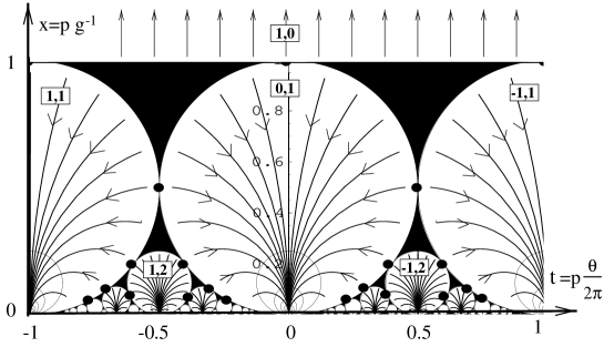
Figure 1: RG flow in the plane $p\frac{\theta}{2\pi},pg^{-1}$. The flow are shown up to $m=3$. The regions inside the circle corresponds to stability regions for charges $(n,m)$ with nonzero $n$, $m$ labelling the size of the circle while $n$ gives their positions. For $pg^{-1}>1$ only charges with $m=0$ exists. The transition points between $m\neq 0$ phases are shown as black points while the black region corresponds to a phase with no charge (neutral phase).

3.3 Analysis of the flow

To derive the phase diagram from the renormalization analysis, we first find the domains where a charge $(n,m)$ proliferate. Such a charge proliferate, or equivalently the parafermion operator (2) associated with a charge $(n+\frac{\theta}{2\pi}m,m)$ is relevant, when the associated fugacity increases under rescaling. From the renormalization eigenvalue of the fugacities in (9jc) we deduce that the pure electric charges $(n,0)$ are relevant only for $x>pn^{2}/4$. For $x<1$ the composites charges $(n,m)$ become relevant inside the circles $[n,m]$ centered on $(t,x)=(-n/m,2/(pm^{2}))$ of radius $2/(pm^{2})$. All this circles are thus tangent to the axis $x=0$ (see figure 1).

Each circle [n,m] is caracterised by a ratio $\nu=n/m$ instead of $n,m$, as all charges $(\lambda n,\lambda m)$ with $\lambda\in\mathbb{Z}$ are generated under renormalization in this circle (see figure 1). In the following we will write $\nu=n/m$ where $m$ is the minimal magnetic charge allowed in the circle. Under renormalization, in a circle $\nu=n/m$, $x=pg^{-1}$ flows to zero while $t$ is renormalized to $t^{*}=\nu$. Hence each rational point of the axis $x=0$ correspond to a fixed point of the RG, caracterising a given phase. The phase $m=0$, stable for $x>pn^{2}/4$, can be viewed as a special circle of infinite radius, caracterised by $\nu=\infty$. In this phase $x\to\infty$ and $t$ is slightly renormalized to a (non universal) real value. Below $x<pn^{2}/4$ and between all these circles, all the fugacities renormalize to zero, which correspond to a neutral phase of the Coulomb gas, caracterised by non universal renormalized $g$ and $\theta$ and vanishing fugacities.

Transitions in this phase diagram are a priori of two different types : the transitions between two circles caracterised by different ratio $\nu$ and the transition between a phase with relevant charge $(n,m)$ and the neutral phase. Transitions of the first kind correspond to tangent points between circles in the phase diagram. Such points exist only when $p=4$. For $p<4$, the circles overlap and these transitions are no more accessible by the present perturbative study, while for $p>4$ all circles with different ratio $\nu$ are disconnected and these transitions disappear. In the following we will consider in more detail the case $p=4$, whose phase diagram is shown on figure 1.

A transition between two phases (ratios) $\nu_{1}$ and $\nu_{2}$ is allowed if the two corresponding circles are tangent to each other, which can be written

$$\nu_{1}-\nu_{2}=\pm\frac{1}{m_{1}m_{2}}$$ (9jl)

The corresponding transition point is located in $(t,x)=(-(n_{1}m_{1}+n_{2}m_{2})/(m^{2}_{1}+m_{2}^{2}),1/(m^{2}_{1}+m_{2}^{2}))$. To analyze further these transitions, we need to remark that any circle $\nu$ can be deduced from the circle $\nu=0$ by succesive application of the transformations $P,P^{-1}$ and the duality $D$. Moreover the circle $\nu=0$ itself is the image under $D$ of the line of phase transitions $x=1$. The transition points between the phase $\nu=0$ and other $\nu^{\prime}=\pm 1/m$ (see figure 1) are all images under $D$ of the transitions points between $[1,0]$ and the phases $[n,1]$, which themselves are related to the transitions $[1,0]\leftrightarrow[0,1]$ by action of $P$ and $P^{-1}$. Thus all the transition points between two ratios $\nu$ and $\nu^{\prime}$ correspond to the same critical behaviour. Similarly all transitions between a phase $\nu$ and the neutral phase (no charge condensate) are images of the transition between $[1,0]$ and this phase. We can now study these two transitions perturbatively in the $y_{n,m}$.

First at a transition between $\nu_{1}=n_{1}/m_{1}$ and $\nu_{2}=n_{2}/m_{2}$ we can write renormalization equations for the distance orthonormal to the transition point $\delta_{12}$ while the distance perpendicular to this axis is not renormalized to lowest order. Using $\epsilon=(m_{1}^{2}+m_{2}^{2})\delta_{12}$ and $y=y_{n_{1}m_{1}},\tilde{y}=y_{n_{2}m_{2}}$ we obtain

$$\partial_{l}\epsilon=2\pi^{2}(y^{2}-\tilde{y}^{2})\quad\quad\quad\quad\partial_{l}y=2\epsilon y\quad\quad\quad\quad\partial_{l}\tilde{y}=2\epsilon\tilde{y}$$

which correspond to a Kosterlitz-Thouless like diverging correlation length $\xi\sim\exp(cte/|\epsilon|^{\frac{1}{2}})$. In both phases, the correlation functions of the parafermion operators decays exponentially :

$$\left<e^{i(n\phi({\bf r})+m\tilde{\phi}({\bf r}))}e^{-i(n\phi({\bf o})+m\tilde{\phi}({\bf o}))}\right>\sim e^{-\frac{r}{\xi}}$$

The transition between the neutral phase and a circle $\nu$ is describe by a critical point with one marginal direction (tangent to the circle) and the same diverging correlation length. While the correlation function have the same kind of exponential decays from the circle side of the transition, they decay algebraically in the neutral phase :

$$\left<e^{i(n\phi({\bf r})+m\tilde{\phi}({\bf r}))}e^{-i(n\phi({\bf o})+m\tilde{\phi}({\bf o}))}\right>\sim\left(\frac{a}{r}\right)^{\frac{1}{x}(n+tm)^{2}+xm^{2}}$$

4 Analogy with the Quantum hall effect

Within the context of the two parameters scaling theory of the quantum hall effect, the first idea consists in identifying the coupling of the Coulomb gas model with the components of the conductivity tensor of the electron gas $\sigma_{xy}=t,\sigma_{xx}=x$. The ratio $\nu$ defined in the above study naturally translate into the filling factors of the quantum Hall states : each circle of the flow diagram correspond to a given quantum Hall fluid and the renormalization equations we obtain provide the expected asymptotic value for this conductivity : $\sigma_{xy}^{*}=\nu,\sigma_{xx}^{*}=0$. Following this analogy we can find that transitions between two filling factors $\nu_{1},\nu_{2}$ are allowed if they satisfy the expected relation (9jl). All the allowed transitions between two plateaux are in the same universality, being related by the duality D (8) which exchange the electric and magnetic charges, as in (?), thus supporting the superuniversality hypothesis(?).

However we notice that in our flow diagram, filling factors with any denominators exist, while only even denominators are expected for quantum hall fluids. Moreover fixed points corresponding to filling factors (circles) with even and odd denominators are related by modular transformations : hence one cannot avoid the even denominators in this model. This result has to be related with recent works (?) which reveal that the symmetry hidden behind the quantum Hall hierarchies should be the subgroup $\Gamma(2)$ of $SL(2,\mathbb{Z})$ instead of the whole modular group. This subgroup is generated by the transformation $z\to-z/(2z+1)$ (instead of $z\to-z^{-1}$ in this study) which preserves the oddness of filling factors. This transformation, when restricted to the axis $t=0$ (imaginary axis), correspond to $g\to g/(1+4g^{2})$. Hence it does not exchange the high and low temperature phases of the usual electromagnetic Coulomb gas(?). Thus an extension of the usual electromagnetic model to a $\Gamma(2)$ invariant theory will not simply correspond to the addition of a topological term as for the model studied in this article.

To conclude, let us comment on the comparison with the recent studies which focus on the constraint on the beta function from the modular symmetry (?). This study (together with (?)) assume a modular (or $\Gamma(2)$) symmetry in a model with two parameters $\sigma_{xx},\sigma_{xy}$, and derive the general form of the beta functions of this model. In our work the model (6) possess an infinite number of coupling constants corresponding to the electromagnetic charge fugacities. Thus a direct comparison between the beta functions is not possible. However it should be noticed that our renormalization procedure provide the first explicit example of the commutation of the modular symmetry and the renormalization, which is the central hypothesis of (?, ?).

5 Conclusion

In this article we thus extended the renormalization study of (?) to the Coulomb gas with a topological $\theta$ term in two dimensions. The renormalization scheme we used provides scaling equations which were found to be themselves invariant under the modular group. To our knowledge this study provide the first example in two dimensions of an explicit renormalization of a modular invariant model. The rich phase diagram of this model certainly deserves more work : of particular interest will be the applications of this renormalization study to the extensions of the various statistical models, related to the electromagnetic Coulomb gas in the absence of the $\theta$ term.

Note added : after completion of this work, a preprint (?) appeared on a related quantum Hall model where a finite electromagnetic background charge is added to the $k=1$ restriction of the model (7) . Although these authors used a simplified scheme, their scaling analysis seem to agree with the complete RG equations we derived in this article.

References

References

- [1]
- [2] [] Boyanovsky D 1989 J. phys. A: Math. Gen. 22, 2601.
- [3]
- [4] [] Burgess C & Lutken C 1997 Nucl. Phys. B 500, 367–378.
- [5]
- [6] [] Callan C & Freed D 1992 Nucl. Phys. B 374, 543.
- [7]
- [8] [] Cardy J 1982 Nucl. Phys. B 203, 17–26.
- [9]
- [10] [] Cardy J & Rabinovici E 1982 Nucl Phys B 203, 1–16.
- [11]
- [12] [] Dolan B 1998 preprint. condmat/9809294.
- [13]
- [14] [] Fradkin E & Kadanoff L 1980 Nucl. Physics B 170, 1–15.
- [15]
- [16] [] Fradkin E & Kivelson S 1996 Nucl. Phys. 474, 543–574.
- [17]
- [18] [] G. Cristofano, D. Giuliano G M & Nicodemi F 1998 preprint. cond-mat/9809344.
- [19]
- [20] [] Georgelin Y, Masson T & Wallet J C 1997 J. Phys. A 30, 5075.
- [21]
- [22] [] Kadanoff L 1978 J. Phys. A 11, 1399–1417.
- [23]
- [24] [] Kadanoff L 1979 Annals of physics 120, 39–71.
- [25]
- [26] [] Kivelson S, Lee D & Zhang S 1992 Phys. Rev. B 46, 223.
- [27]
- [28] [] Laughlin R 1983 Phys. Rev. Lett. 50, 1395–1398.
- [29]
- [30] [] Lütken C & Ross G 1992 Phys Rev B 45, 11837.
- [31]
- [32] [] Nienhuis B 1987 in C Domb & J Leibowitz, eds, ‘Phase Transition and Critical Phenomena’ Vol. 11 Academic Press (London).
- [33]
- [34] [] Pryadko L & Zhang S 1996 Phys. Rev. B 54, 4953
- [35]
- [36] [] Shahar D, Tsui D, Shayegan M, Shimshoni E & Sondhi S 1996 Science 274, 589.
- [37]
- [38] [] Shapere A & Wilczek F 1989 Nucl Phys B 320, 669–695.
- [39]
- [40] [] Villain J 1975 Jour. de Phys. (France) 36, 581.
- [41]