Enumeration of States in a Periodic Glass

Abstract

We present an analytic enumeration of the metastable states, $N_{s}$, in a periodic long-range Josephson array frustrated by a transverse field. We find that the configurational entropy, $S_{conf}\equiv\ln N_{s}$, is extensive and scales with frustration, confirming that the non-random system is glassy. We also find that $S_{conf}$ is different from that of its disordered analogue, despite that fact that the two models share the same dynamical equations.

The problem of vitrification has been studied for many years and remains a topic of much current interest [1]. Recently there has been significant progress in our conceptual understanding of glass formation in the absence of quenched disorder due to studies of exactly soluble models [2, 3, 4, 5, 6, 7]. Many features of these regular microscopic systems are the same as those of known disordered Hamiltonians [8]. More specifically, the dynamical equations of these periodic glasses are identical to those of (intrinsically random) spherical spin glass models; many signatory properties such as history-dependence and ageing follow from these equations. These results suggest that one can study periodic glasses via a mapping to disordered ones for which analytical tools are well-developed [9, 10]. Here, however, we show that some physical properties of periodic and disordered models which share the same dynamical equations are different. In particular we have calculated the number of metastable states, $N_{s}$, with different ordering of the superconducting phases in a periodic long-range Josephson array. We find that the configurational entropy, $S_{conf}\equiv\ln N_{s}$, is extensive proving that this system is indeed in a glassy phase. However, $S_{conf}$ in this model is distinct from the configurational entropy of its disordered counterpart, despite the fact that they share the same dynamical equations.

We shall consider the following periodic model, which has the advantage that it can be studied both analytically [6, 11] and experimentally [12, 13]. The proposed array is a stack of two mutually perpendicular sets of $N$ parallel wires with Josephson junctions at each node that is placed in an external tranverse field, $H$. The classical thermodynamic variables of this system are the superconducting phases associated with each wire. Here we shall assume that the Josephson couplings are sufficiently small so that the induced fields are negligible in comparison with $H$. We can therefore describe the array by the Hamiltonian

$${\cal H}=-\sum_{m,n}^{2N}z_{m}^{*}\ {\cal J}_{mn}\ z_{n}$$ (1)

where ${\cal J}_{mn}$ is the coupling matrix

$$\hat{{\cal J}}=\left(\begin{array}[]{cc}0&\hat{J}\\ \hat{J}^{\dagger}&0\end{array}\right)$$ (2)

with $J_{jk}=\frac{J_{0}}{\sqrt{N}}\exp(2\pi i\alpha jk/N)$ and $1\!\leq\!(j,k)\!\leq\!N$ where $j(k)$ is the index of the horizontal (vertical) wires; $z_{m}=e^{i\phi_{m}}$ where $1\leq m\leq 2N$ and the $\phi_{m}$ are the phases associated with the superconducting order parameters of the $2N$ wires. Here we have introduced the flux per unit strip, $\alpha=NHl^{2}/\Phi_{0}$, where $l$ is the inter-node spacing and $\Phi_{0}$ is the flux quantum; the normalization has been chosen so that $T_{G}$ does not scale with $N$.

Because every horizontal (vertical) wire is linked to every vertical (horizontal) wire, the number of nearest neighbors in this model is $N$; we can therefore study it with a mean-field approach. Such an analysis of the thermodynamic properties indicates that at sufficiently low temperatures the paramagnetic phase becomes unstable with $\alpha N$ modes becoming simultaneously degenerate[6]. We speculated previously that any linear combination of these modes would result in a metastable state at lower temperatures leading to $S_{conf}\sim\alpha N$. The results of the explicit calculation described below confirm this conjecture.

In the limit of small transverse field $(\frac{1}{N}<\alpha<1)$, the dynamical equations of the periodic array are identical to those of the $p=4$ (disordered) spherical spin glass model [11]. These equations indicate that all metastable states are formed at the transition, with no further subdivision occurring at lower temperatures [14]. This conclusion agrees with that found from a direct study of the TAP solutions of the $p=4$ spherical spin glass model [15]. It is thus sufficient to calculate the number of states, $N_{s}$, in the periodic model at zero temperature. Because there is no average over disorder in this regular array, there is no distinction between $\ln\langle N_{s}\rangle$ and $\langle\ln N_{s}\rangle$ as occurs for intrinsically random systems, and hence no corresponding problems of relevance or interpretation of $\ln\langle N_{s}\rangle$ that one usually calculates instead of the more physical $\langle\ln N_{s}\rangle$.

At zero temperature the defining characteristic of a metastable state is that each spin should be parallel to its associated molecular field [16]. This physical condition results in a highly nonlinear equation which determines the number of states. Previous studies of disordered $xy$ spin systems indicate that the crucial nonlinearities appear in the expression for the amplitude, due to the quasi-linear nature of the phase component. More specifically, the configurational entropy for the $xy$ Sherrington-Kirkpatrick model[17] is different from that of its Ising counterpart by a numerical factor of $O(1)$. This observation allows one to reduce the array problem to that of Ising spins, $s_{m}=\pm 1$, thereby simplifying the technical presentation. In this case, the number of states is given by

$$N_{s} \equiv {\rm{Tr}}_{s}\prod_{m}\theta\left(s_{m}\sum_{n}{\cal J}_{mn}s_{n}\right)$$ (3)

$$= \int^{+\infty}_{-\infty}{\cal D}\phi\hskip 3.61371pt{\rm{Tr}}_{s}\hskip 3.61371pte^{i\sum_{mn}{\cal J}_{mn}{\cal A}_{mn}s_{m}s_{n}}$$ (4)

where we have used an integral representation of the $\theta$-function, ${\cal D}\phi\equiv{\prod_{m}\frac{{\it{d}\phi_{m}}}{2\pi i\phi_{m}}}$ and ${\cal A}_{mn}\equiv(\phi_{m}+\phi_{n})$.

We use the cumulant expansion to determine the integral (4). Since only terms with an even power of each spin variable contributes to this sum, it can be represented as a closed loop product of $(J{\cal A})_{ij}$ matrices. Moreover the structure of the periodic array is such that only loops containing an even product of these matrices are possible [6, 19]. For the explicit calculation we shall need the moments of the couplings $\langle J^{2p}\rangle$. We know from previous work on the array [6, 19] that

$$\langle J^{2p}\rangle = \left(\frac{1}{N^{2p-1}}\right)\lim_{N\rightarrow\infty}\sum_{i_{1},j_{1},i_{2}...j_{p}}J_{i_{1}j_{1}}J_{j_{1}i_{2}}\hskip 0.72229pt...\hskip 0.72229ptJ_{j_{p}i_{1}}$$ (5)

$$= \frac{1}{\alpha^{p-1}N^{2p-1}}$$ (6)

where $J_{0}\equiv 1$; this result can be understood physically since only horizontal (vertical) wires separated by $d<l/\alpha$ contribute coherently to this sum independent of disorder. We emphasize that so far our calculation can be applied to both periodic and random arrays; the only difference is that in the latter case the couplings are averaged over disorder.

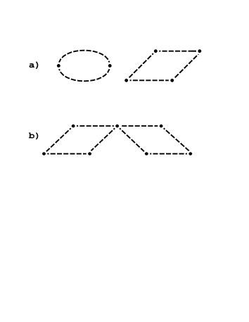
FIG. 1.: Diagrams for the spin trace: (a) Closed non-intersecting loops that give the main contribution to $N_{s}$ in the limit $\alpha\ll 1$ and (b) Intersecting loops that are next order in $\alpha$.

The summation over spin variables in (4) can be graphically represented by the sum of diagrams with closed loops, shown in Fig. 1. Diagrams with intersecting loops (see Fig. 1) are small in $\alpha$ due to the structure of the moments (6); thus we can neglect such diagrams for $\alpha<1$ which simplifies the problem. Furthermore each closed loop diagram, (see Fig. 1a), makes a contribution $K^{2p}=\int{\cal D}\phi\ {\rm{Tr}\ ({\cal JA})^{2p}}$ to (4) where $p$ refers to the number of nodes in the graph. The integration over the phase variables makes all sites equivalent, so that $K^{2p}=\langle{\cal J}^{2p}\rangle\int{\cal D}\phi\ {\rm{Tr}\ {\cal A}^{2p}}$. Summing all the loop diagrams and rescaling $\phi\rightarrow\sqrt{\alpha}\phi$, we have

$${N_{s}}=2^{N}\int{\cal D}\phi\hskip 1.4457pte^{\alpha N{\cal S}(\phi)}\hskip 8.67204pt,\hskip 8.67204pt{\cal S}(\phi)=\sum_{p}\frac{(-1)^{2p}}{(2p)N^{2p}}{\rm{Tr}\hskip 1.4457pt{\bf A}^{2p}.}$$ (7)

More explicitly, because ${\cal A}_{ij}=(\phi_{i}+\phi_{j})$

$$\mbox{Tr}\ {\bf A}^{n}\equiv\sum_{i_{1},\ldots i_{n}}(\phi_{i_{1}}+\phi_{i_{2}})(\phi_{i_{2}}+\phi_{i_{3}})\ldots(\phi_{i_{n}}+\phi_{i_{1}}).$$ (8)

In each term of the resulting polynomial each index is represented zero, one or at most two times; the resulting contributions to $\frac{1}{N^{n}}{\rm Tr}{\bf A}^{n}$ are $\frac{1}{N}\sum_{i}1\equiv 1$, $\frac{1}{N}\sum_{i}\phi_{i}$ and $\frac{1}{N}\sum_{i}\phi_{i}^{2}$ respectively. Therefore $\frac{1}{N^{2p}}{\rm Tr}{\bf A}^{2p}$ is a function of only $t\equiv\frac{1}{N}\sum\phi$ and $u\equiv\frac{1}{N}\sum\phi^{2}$. In order to calculate $\mbox{Tr}{\bf A}^{n}$ explicitly, we separate the two terms in which each index appears once and only once from those in which some indices are repeated and others do not appear at all. Furthermore, it is convenient to compute the second term via its derivative:

$$\mbox{Tr}\ {\bf A}^{n}=2t^{n}+\int_{0}^{u}\frac{\partial\mbox{Tr}{\bf A}^{n}}{\partial u}du.$$ (9)

Explicitly the derivative in the second term is given by

$$\frac{\partial\mbox{Tr}\ {\bf A}^{n}}{\partial u}=nNC_{n-2}$$ (10)

$$C_{n}=\sum_{i_{1},\ldots i_{n+1}}(\phi_{i_{1}}+\phi_{i_{2}})(\phi_{i_{2}}+\phi_{i_{3}})\ldots(\phi_{i_{n}}+\phi_{i_{n+1}}).$$ (11)

Here $C_{n}$ can be determined recursively, once again separating into terms which involve only distinct and repeated indices. Explicit computation of the sum in equation (7), involving some algebra, yields

$${\cal S}=-\frac{1}{2}\ln\left\{(1+t^{2})^{2}+2u(1-t^{2})+u^{2}\right\}.$$ (12)

Because ${\cal{S}}$ depends on $\phi$ solely via $t$ and $u$ defined above, the $N$-dimensional integral over $\phi$ in (7) can be conveniently calculated by including two additional integrals over $t$ and $u$, and the factors $\delta\left(t-\frac{1}{N}\sum\phi\right)$ and $\delta\left(u-\frac{1}{N}\sum\phi^{2}\right)$.

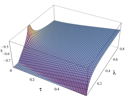
FIG. 2.: ${\cal S}(\tau,\lambda)$ for a typical $\alpha$ ($\alpha=0.1$) which displays the saddle-point.

We may use the integral representation of the $\delta$-functions and integrate over each $\phi_{i}$ independently; the result can be concisely presented using the function $\Theta(x)\equiv\frac{1}{2}\left\{1+{\rm{Erf}(\frac{x}{2})}\right\}$ so that the integral in (7) becomes

$${N_{s}}=2^{N}\int^{i\infty}_{-i\infty}\!d\lambda\!\int^{\infty}_{-\infty}\!dt\ du\ d\tau\hskip 3.61371pte^{N\left\{\alpha{\cal{S}}+i\tau t+\lambda u+\ln\Theta\left(\frac{\tau}{\sqrt{\lambda}}\right)\right\}}$$ (13)

where ${\cal{S}}$ is given by (12). The factor of $N$ in the exponential of the integral in (13) allows us to evaluate this integral by a saddle-point approximation. We shift our contour in $t$ by $i\tilde{t}$ to look for a solution, since on physical grounds we expect the saddle-point to be real. This is indeed the case, as displayed in Figure 2, and the result is

$$S_{conf}\equiv\ln N_{s}=\frac{N\alpha}{2}\ln\frac{1}{2\alpha}.$$ (14)

for $\alpha\ll 1$. This equation for the configurational entropy is the main result of this paper. It indicates that $S_{conf}$ is extensive, as expected for a glass. Furthermore $S_{conf}$ is proportional to $\alpha N$, consistent with the fact that there is vanishing frustration in the limit of $\alpha\leq\frac{1}{N}$. Physically, we note that the configurational entropy in (14) is proportional to the effective number of spins $\alpha N$ in the periodic model; in this array, phases (and hence spins) are correlated on a length-scale $\frac{l}{\alpha}$ where $l$ is the internode spacing. Eq. (14) also concurs with a conjecture based on a previous stability analysis for the high temperature paramagnetic phase [6].

The calculation above can be generalized to find the number of states in which all molecular fields are greater than a threshold value, $h_{th}$. For small $h_{th}$ the associated configurational entropy decreases as $\delta S_{conf}\sim-N\alpha^{1/2}h_{th}$. We note that both $S_{conf}$ and $\delta S_{conf}$ are proportional to $N$. Empirically we believe that states in which some spins experience a very small molecular field are only marginally stable. Thus this perturbative change in the configurational entropy induced by finite $h_{th}\ll 1$ implies that in the thermodynamic limit the number of marginal states is extensive.

We can also extend this calculation to determine the number of states as a function of their energy. To do this we introduce an additional $\delta(NE-\sum_{mn}{\cal J}_{mn}s_{m}s_{n})$ function in the definition (3) which extracts only states with energy $E$. Using an integral representation of this $\delta$ function with an additional variable $\mu$ we see that ${\cal D}\phi$ in Eq (4) becomes ${\cal D}\phi=\Pi_{m}\frac{d\phi_{m}}{2\pi i(\phi_{m}+\mu)}$ and the exponential acquires an additional contribution $iN\mu E$. Finally in the final integral (13) the exponential acquires the term $iNE\mu$ and function $\Theta(\tau/\sqrt{\lambda})$ is replaced by

$$\tilde{\Theta}(\tau,\lambda) = \int\frac{d\phi}{2\pi i(\phi+\mu)}e^{-\lambda\phi^{2}+i\tau\phi}$$ (15)

$$= e^{-\mu^{2}\lambda-i\tau\mu}\Theta\left(\frac{\tau-2i\mu\lambda}{\sqrt{\lambda}}\right)$$ (16)

We evaluate the resulting integral by a saddle-point approximation. Three out of the five resulting saddle-point equations can be solved analytically; the remaining two contain an error function and must be solved numerically.

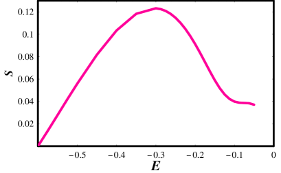
FIG. 3.: ${\cal S}_{conf}(E)$ for $\alpha=0.1$

Our numerical solution for the configurational entropy as a function of energy is displayed in Figure 3 for $\alpha=0.1$. Qualitatively it is similar to the behavior of $S_{conf}(E)$ for spin glasses with intrinsic randomness[16, 17, 18]. However its analytical structure is distinct, specifically from that of the $p=4$ (disordered) spherical model [18]. Furthermore all states displayed in Fig. 3 are stable, whereas in the $p$-spin model all states above a certain threshhold energy are unstable. We note, however, that here we are only considering stability with respect to single-spin flips; by contrast in the $p$-spin model stability is defined with respect to continuous deformations.

The result (14) was derived in the limit of small $\alpha$, and we have also checked the qualitative validity of our conclusion for $\alpha=1$ with $xy$ spins using a different method than that discussed above. We emphasize that the $\alpha=1$ case is very special, since in this instance $J_{ij}$ is a unitary matrix. Furthermore we note that for $\alpha=1$ the coupling matrix $J_{ij}$ is identical to a discrete Fourier transform; then the condition that the Fourier transform is flat defines a stable spin configuration. It is convenient to write this condition as $B_{r}\equiv{\sum_{k=0}^{N}z^{*}_{k}z_{k+r}}$ equals zero for $r\neq 0$. Then we obtain the equation for the number of states

$${N_{s}}=\int\prod_{r=1}^{N}dz_{r}\hskip 3.61371ptdz^{*}_{r}\hskip 3.61371pt\frac{\delta(|z_{r}|-1)}{2\pi}\hskip 3.61371pt\delta(B_{r})\hskip 3.61371pt\det\frac{\partial B}{\partial z}.$$ (17)

Since the $B_{r}$ are pseudo-random variables with $\langle B^{2}\rangle=N$ we may assume that they obey a Gaussian distribution with $P(B)\approx\frac{1}{2\pi N}e^{-}\frac{|B^{2}|}{N}$. The determinant in (17) can be evaluated exactly by noting that $\frac{\partial B_{k}}{\partial z}=z^{*}_{i+k}$ implying that for $z$’s that satisfy the condition $B_{r}=0$ all rows are orthogonal. The length of each row is $N$ so that the determinant $|\frac{\partial B}{\partial z}|=N^{N}$. Therefore the average over $B$ in (17) results in

$$S_{conf}\equiv\ln N_{s}=N\ln\sqrt{\frac{N}{2\pi}}.$$ (18)

This expression was derived in the limit of $N\gg 1$; from its form it is clear that this asymptotic result can be attained only at numerically large $N$ (at least $N\gg 2\pi$). In order to check the behavior of $S_{conf}$ for $\alpha=1$ at moderate $N$, we have performed a direct numerical minimization of the Hamiltonian in (1); the results, displayed in Fig. 3, clearly indicate that the configurational entropy is extensive. We expect that $S_{conf}$ crosses over from $S_{conf}\approx N\ln 2$ (obtained numerically as shown in Fig. 3) to the analytical result (18) at $N\approx 20$; however from a practical standpoint this crossover is inaccessible numerically due to the extensive nature of the ground-state manifold.

To summarize our results, we have calculated the number of states in a periodic glass and have found that the configurational entropy, $S_{conf}=\ln N_{s}$, is proportional to $\alpha N$ (Eq. (14)). It is thus extensive but is different from that of the $p=4$ (disordered) spherical spin glass model [7] despite the fact that their dynamical equations are identical [11, 14]. Furthermore, the complexities (the number of states as a function of energy) of these two models have different functional forms. It appears that rather different microscopic models can have the same dynamical behavior, as evidenced by the fact that the parameter $\alpha$ (for $\alpha<1$) does not affect the rescaled response. As an aside, we note that $S_{conf}$ for the disordered array is also distinct from that of the Sherrington-Kirkpatrick model, even though they share the same dynamics [19]; however $S_{conf}$ for the periodic and the random networks are identical, which may be coincidental. These qualitative results remain valid for $\alpha=1$, thus suggesting that they are independent of our approximation given the absence of commensurability. We note, however, that the dynamical equations change their form at $\alpha\sim 1$, and become similar to those of disordered spherical spin glass models with interactions that are sums of couplings with $p\geq 4$; qualitatively this does not seem to affect the number of states.

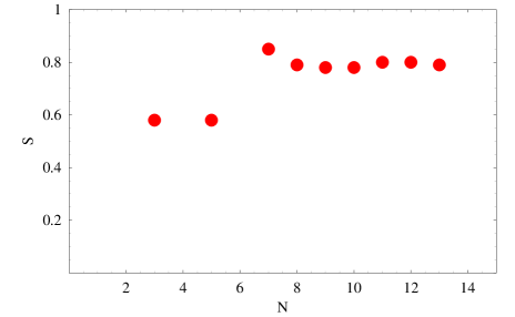
FIG. 4.: Numerical results for the configurational entropy, $s\equiv S_{conf}/N$, for $\alpha=1$ as a function of $N$. Note that for $N<12$ the possible error is less than the size of the points.

The fact that the periodic long-range array and the $p=4$ spherical (disordered) spin glass have different configurational entropies suggests that the detailed structure of their respective phase spaces, e.g. barriers, basins of attraction, is quite distinct. This is not inconsistent with previous work which indicates that these two models share the same dynamical equations[11, 14]. The latter were derived in the thermodynamic limit ($N\rightarrow\infty$), and do not describe transitions between metastable states that might occur at finite $N$. Thus these equations only probe the system’s responses in the vicinity of a typical state where it is trapped, and are insensitive to the total number of metastable configurations. The distinction between the configurational entropies of the periodic and disordered models indicates differences in their physical properties at finite $N$ and, most likely, in the characteristics of analogous finite-range systems. We therefore believe that a detailed study of the structure of their respective phase spaces could give insight about the physics of finite-range problems and about differences between disordered and structural glasses.

Experimentally states are accessed with some weighing factor which is ignored by the quantity $N_{s}$ calculated here; for example in thermal equilibrium they would be weighted with a Boltzmann factor, whereas in a rapid quench they would be weighted according to the size of their basins of attraction. Furthermore it seems likely [20] that the distribution of the basins of attraction is broad; if so, some states would have weights much larger than others in a rapid quench. Nonetheless we believe that the main conclusion of this paper remains valid; the number of states can be very different for systems which share the same dynamical equations.

We thank D.S. Fisher for raising the issue of stability of the states. P.C. acknowledges the hospitality of the Department of Physics and Brasenose College during a sabbatical leave at Oxford. L.I. is grateful to the same Physics Department and to New College (Oxford) for their support during the period of this research. The work performed at Oxford University was partially funded by the UK EPSRC under grant DR 8729.

REFERENCES

- [1] For an overview of the structural glass problem see Science, 267, 1924-1953 (1995) for a series of articles by C.A. Angell; F.M. Stillinger; B. Frick and D. Richter; I.M. Hodge; and A.L. Greer.
- [2] J.P. Bouchaud and M. Mezard, J. Physique 4, 1109 (1994)
- [3] E. Marinari, G. Parisi and F. Ritort, J. Phys. A27, 7647 (1994); E. Marinari, G. Parisi and F. Ritort, J. Phys. A28 327 (1995).
- [4] L. Cugliandolo, J. Kurchan, G. Parisi and F. Ritort, Phys. Rev. Lett. 74, 1012 (1995).
- [5] S. Franz and J. Hertz, Phys. Rev. Lett. 74, 2114 (1995).
- [6] P. Chandra, L.B. Ioffe and D. Sherrington, Phys. Rev. Lett. 75, 713 (1995).
- [7] Recent developments are reviewed in J-P. Bouchaud, L. Cugliandolo, J. Kurchan and M. Mezard in Spin Glasses and Random Fields (Directions in Condensed Matter Physics Vol. 12),A.P. Young ed. (World Scientific, Singapore, 1997).
- [8] The mapping between periodic and disordered systems was first suggested in T.R. Kirkpatrick and D. Thirumalia, Phys. Rev. Lett. 58, 2091 (1987); T.R. Kirkpatrick and D. Thirumalai, Phys. Rev. B 36, 5388 (1987) T.R. Kirkpatrick, D. Thirumalai and P.G. Wolynes, Phys. Rev. A 40, 1045 (1989).
- [9] J.-P. Bouchaud, L. Cugliandolo, J. Kurchan and M. Mezard, Physica A226, 243 (1996).
- [10] G. Parisi in Complex Behaviour of Glassy Systems, eds. M. Rubi and C. Perez-Vicente (Springer-Verlag, Berlin, 1997) pp. 111-121.
- [11] P. Chandra, M.V. Feigelman and L.B. Ioffe, Phys. Rev. Lett. 76, 4805 (1996).
- [12] P. Chandra, M.V. Feigelman, M.E. Gershenson and L.B. Ioffe in Complex Behaviour of Glassy Systems, eds. M. Rubi and C. Perez-Vicente (Springer-Verlag, Berlin, 1997) pp.376-384.
- [13] H. Shea and M. Tinkham, Phys. Rev. Lett. 79, 2324 (1997).
- [14] P. Chandra, M.V. Feigelman, L.B. Ioffe and D.M. Kagan, Phys. Rev. B 56, 11553 (1997).
- [15] J. Kurchan, G. Parisi and M.A. Virasoro, J. Phys. I 3, 1819 (1993).
- [16] F. Tanaka and S.F. Edwards, J. Phys. F. 10,1769 (1980); A.J. Bray and M.A. Moore, J. Phys. C 13,L469 (1980); C. De Dominicis, M. Gabay, T. Garel and H. Orland, J. Physique 41, 923 (1980).
- [17] F. Tanaka and S.F. Edwards, J. Phys. F.10,2779 (1980); A.J. Bray and M.A. Moore, J. Phys. C 14, 2629 (1981).
- [18] A. Crisanti and H.J. Sommers, J Phys. I France 5, 805 (1985); S. Franz and G. Parisi, J. Phys. I France 5, 1405 (1995); A. Cavagna, I. Giardina and G. Parisi, Phys. Rev. B 57, 11251 (1998).
- [19] V.M. Vinokur, L.B. Ioffe, A.I. Larkin and M.V. Feigelman, Sov. Phys. JETP, 66, 198 (1987).
- [20] P. Chandra and L.B. Ioffe, to be published.